Abstract
This numerical study demonstrates the existence of a critical injection momentum threshold necessary for stable liquid film formation, highlighting that either excessive or insufficient momentum degrades cooling performance. This optimization is critical for maximizing cooling effectiveness from short injection holes in high-performance propulsion systems. By comparing Smoothed Particle Hydrodynamics (SPH) and Volume of Fluid (VOF) methods, we find that the SPH method predicts a thicker, more continuous coolant film due to its superior mass conservation during interface breakup. A key design insight emerges: cooling performance peaks at a distinct, critical coolant momentum. Insufficient momentum leads to poor coverage, while excess momentum causes film separation and is counter-productive. The identified configuration—defined by a precise combination of flow rate, pressure, and geometry—promotes immediate and stable film formation. The robustness of this finding is confirmed by the agreement between the two numerical methods on film thickness and the captured physical evolution of the film from a pronounced wave to a damped state.
1. Introduction
Aerospace vehicles traveling at hypersonic velocities (defined as exceeding Mach 5), such as scramjets, must withstand a severe thermal environment and extreme aerodynamic and thermal stresses [1,2]. Notwithstanding these considerations, the severe aero-thermal environment imposes significant constraints on the vehicle’s material selection and structural design. To manage the intense heat generated during hypersonic flight, thermal protection systems must employ innovative injectors, high-performance coolants, and meticulously engineered designs [3]. Similarly, the push for more powerful and efficient gas turbine engines necessitates higher operating temperatures, a goal shared by modern turbine manufacturing. However, these intense temperatures place immense thermal stress on the turbine blades [4]. To enhance thermal efficiency and thermodynamic performance, a primary approach is to increase the turbine inlet temperature (TIT) [5,6]. Consequently, at a constant pressure ratio, the net energy output increases and rotor blade performance improves, a result explained by thermophysics principles [3]. Film cooling is a critical thermal protection method for systems such as hypersonic vehicles and core engine components like turbine blades and combustion chambers. While the broader aim of the associated research program is to inform the optimization of combustion chamber design, this requires a foundational understanding of fundamental cooling parameters—including blowing ratios [7], coolant Mach number [8], shockwave [9] interactions, and injector orientations [10]. Therefore, the immediate focus of this paper is to establish controlled foundational data for film cooling on an external flat surface under high-speed, high-temperature flow conditions. This simplified, canonical geometry allows for the isolation and systematic study of key physics, the results of which provide essential validation data for models that can subsequently be applied to complex internal geometries like combustion chambers. The flat-plate configuration employed for the boundary layer transition analysis is shown schematically in Figure 1.
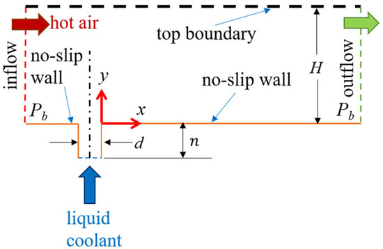
Figure 1.
Schematic of the Flat-Plate setup used for boundary layer transition analysis.
Initial investigations into film cooling were largely centered on various techniques, notably cooling via slots [11,12,13] and cylindrical holes, as well as the role of the injection angle [14,15,16]. The review by Umana and Yang [3] characterizes the film cooling mechanism by the interaction of the mainstream and secondary fluids. The exploration of shaped film-cooling holes, including fan-shaped and laid-back fan-shaped geometries, was enabled by advancements in manufacturing technology and has been the subject of studies by several authors [17,18,19,20]. While prior research consistently demonstrates the enhanced cooling performance of shaped holes relative to cylindrical holes, later work expanded this exploration to advanced geometries [21]. Specifically, Dhungel et al. [22] investigated branched holes, while Yiping et al. [23,24] studied trenched cylindrical holes, both of which reported improved film-cooling effectiveness. In their hydrodynamic analysis, Burd et al. [25] investigated short film-cooling holes (L/D = 2.3) against a long-hole baseline (L/D = 7) under fixed conditions (35° injection, density ratio = 1.0) and across Free-Stream Turbulence Intensity (FSTI) levels of 0.5% and 12%. The study concluded that while short holes promote a jetting behavior in the secondary fluid, this effect is significantly mitigated at high turbulence intensities, leading to a diminished distinction between short and long hole performances.
The experimental work by Ligrani and Bell [26] examined the interplay of density ratio (DR: 0.94–1.4), hole length-to-diameter ratio (L/D: 3, 4), and pulsation frequency (0, 8, 20 Hz) at a fixed 35° injection angle. Their results indicated that while L/D had an insignificant effect at low DR without pulsation, an L/D of 4 outperformed an L/D of 3 at high DR under steady flow. Notably, increasing the pulsation frequency to 20 Hz reversed this performance trend. Gritsch et al. [27] conducted a parametric study on fan-shaped holes, examining the effects of inlet-to-outlet area ratio, coverage ratio, pitch ratio, length (L/D = 7.5, 9.5, 11.5), and compound angle. With carbon dioxide as the secondary fluid (density ratio = 1.7), their results showed that film-cooling effectiveness was largely insensitive to L/D and coverage ratio but highly sensitive to pitch-to-diameter ratio and orientation angle. In an experimental study on a flat plate, Wilfert and Wolff [28] found that long cooling holes (L/D = 8) provided better cooling than short holes (L/D = 4) for a row of cylindrical holes oriented at 30°, a conclusion drawn from testing five different plenum geometries. Hale et al. [29] corroborated this finding, demonstrating in their comparison of L/D ratios from 0.66 to 3.0 that a 90° injection angle can achieve film-cooling effectiveness comparable to a 35° angle at high blowing ratios.
In their investigation of the length-to-diameter (L/D) ratio’s effect on film cooling, Lutum and Johnson [30] injected secondary air (density ratio = 1.15) at 35° through cylindrical holes. They examined blowing ratios from 0.52 to 1.56 across five L/D ratios (1.75, 3.5, 5, 7, 18), categorizing L/D = 1.75 and 3.5 as ‘short’ holes and the higher ratios as ‘long’ holes. This computational study examines the morphology of a flat-plate boundary layer, focusing on the case of a short cylindrical hole (L/D ≤ 3) [21] and a liquid film injected at a 90° angle. While turbine blades are thick enough to incorporate shaped cooling holes, thinner components, such as the combustion chambers and afterburners in fighter aircraft, are restricted to short cylindrical holes. Despite the extensive literature on film cooling, this specific and practical configuration has received limited attention.
1.1. Film Cooling Using a Liquid Jet
The efficacy of liquid film cooling is fundamentally distinct from gaseous cooling, enhanced by the working fluid’s inherent thermal properties—namely, a higher specific heat and the absorption of latent heat during evaporation. Furthermore, the vapor produced does not immediately dissipate into the crossflow. It adheres to the surface, forming a stable, protective barrier that significantly prolongs the cooling effect in the streamwise direction [3].
The field of liquid film cooling has seen substantial advancement. Its application is well-documented in aerospace engineering, particularly for cooling rocket engine combustion chambers operating under specified pressures and mixture ratios [31]. Experimental investigations have utilized controlled percentages of various coolants, such as water, ethyl alcohol, and liquid ammonia. Performance has been studied in systems using both conventional and cryogenic-storable propellants [32], with detailed quantitative heat transfer analysis. Furthermore, studies have experimentally determined how injector geometry [33] and the blowing ratio influence cooling efficiency, affecting both film coverage and thermal uniformity downstream of injection.
A series of experimental studies has examined the performance of tangential liquid film injection. Morrell [31] compared vertical and 45° tangential slot injectors, finding no cooling effectiveness advantage for the tangential orientation. In a nickel calorimetric chamber, Kesselring et al. [32] used tangential injectors to identify key design factors. Their analysis, which employed data simplification techniques for short-duration tests, suggested the liquid film evaporated abruptly, as inferred from heat flux calculations without transpiration. Expanding the investigation to cylindrical holes, Shine et al. [33] compared tangential and multi-angle configurations through combined experimental and computational methods. They found that adding a compound angle did not improve cooling over simple tangential injection and, notably, resulted in a shorter liquid film length. This body of work reinforces a common design feature: coolant holes are most frequently angled tangentially to the hot gas flow [3].
A series of studies has advanced the understanding of liquid film cooling in high-intensity environments like rocket engines. First, an experimental investigation of film cooling under high-momentum turbulent flow led to a technique for calculating the evaporation rate and surface temperature behind a uniform thermal barrier [34]. Focusing on rocket combustion chambers specifically, Zhang et al. [35] employed a coupled numerical approach. They simulated coolant turbulence with a van Driest model and mainstream gas flow with a heat transfer model to analyze the effects of flow characteristics and coolant properties. Their in-depth parameter study, which showed good agreement with experiments, quantified how these factors influence the cooled film length. Further optimizing thermal protection, another study examined entrainment and reacting films in swirling flows within combustion chambers [36]. The findings demonstrated that such configurations can reduce entrainment and maintain manageable wall temperatures, highlighting the performance potential of controlled swirling.
1.2. Instability and Rupture of the Thin Film
Liquid films flowing over a heated surface are prone to thermocapillary instabilities. These instabilities are generated by shear stresses that result from surface tension variations with temperature—a phenomenon known as the Marangoni effect. This process can induce film rupture, creating dry areas on the heated surface. Consequently, a thorough understanding of the rupture mechanisms is crucial for maintaining a stable, continuous film flow and preventing the formation of dry spots [37]. Thin liquid films exhibit complex and fascinating dynamical behaviors. Their deformable liquid-gas interface supports wave propagation, which can intensify and travel at high flow rates. These waves may further evolve into quasiperiodic or chaotic states. Under certain conditions, the film may rupture, forming holes that reveal the underlying substrate and alter the film’s continuity. Similarly, film fragmentation—where droplets detach—also disrupts its connectivity. Additionally, in flows involving contact lines, structural changes can produce distinctive fingered patterns [38]. An experimental study was performed to investigate three-dimensional (3D) instabilities in falling films on an inclined plane, with flow driven at the upstream end. The aim was to understand the transition from two-dimensional (2D) waves to complex disordered patterns [39]. The authors concluded that 2D disturbances initially grow more rapidly than 3D ones, leading to the first excitation of 2D waves with straight fronts. They also discovered that the nonlinear evolution of the waves depends on the frequency of the small perturbations driving the flow. Similarly, an experimental study on the rupture dynamics of a horizontally oriented liquid film, non-uniformly heated from below, was conducted across a wide range of liquid viscosities [37]. The angular and frequency characteristics of a confocal sensor were examined in detail. The film rupture process was divided into three stages: (1) thinning down to a residual film on the heater; (2) the existence of a stable residual film for a period; and (3) the rupture and dry-out of this residual film. The researchers found that the thickness of the residual film strongly depends on the liquid viscosity: for water, it is approximately 10 μm, while for the more viscous silicone oil (PMS-200), it is about 275 μm.
Thermocapillary-driven rupture of liquid films has been widely investigated under diverse configurations. These include: a stationary horizontal layer heated non-uniformly from below [40,41]; a flowing film over a horizontal plate with a local heat source [42]; a gravity-driven film on a vertical plate with local heating [43,44]; and a stationary horizontal layer heated from above by a focused laser beam [45]. Research demonstrates that decreasing the liquid layer’s thickness or the flow rate destabilizes the film, making it more susceptible to rupture and dry spot formation. This rupture process is complex, involving thickness changes spanning several orders of magnitude—from millimeters down to micrometers or even nanometers. Within this scale transition, different physical forces become dominant at different stages. Furthermore, film rupture is intrinsically linked to the physics of the contact line [46,47,48], which governs the behavior of a dry spot after it nucleates. Pioneering work [49] first revealed that for a distilled water film, thermocapillary rupture involves an intermediate stage where a thin residual film coats the heater surface before a dry spot fully forms [37].
1.3. Heat Transfer During Liquid Film Phase Change
Understanding heat and mass transfer within evaporating thin films is essential for designing high-performance micro-scale phase-change devices like capillary-assisted evaporators, heat pipes, and vapor chambers. Therefore, accurate modeling of these processes is critical for effective device design [50]. The capillary pressure generated by interfacial curvature and surface tension, combined with disjoining pressure gradients, supplies the thin-film transition region (1–100 nm thick). This supply facilitates exceptionally high heat transfer rates under low superheat conditions [51].
Significant research efforts have focused on modeling heat transfer within the thin-film region. Early foundational work by Potash and Wayner [52] established that liquid flow in this region is driven by a disjoining pressure gradient. Building on this, Wayner et al. [53] derived and numerically solved a governing equation for the film profile by equating the liquid mass flux to a simplified version of Schrage’s kinetic theory-based evaporative mass flux expression [54], neglecting evaporative suppression from capillary pressure in their analysis. Schonberg and Wayner [55] advanced the model by developing an expression for the thin-film mass flow rate and providing an analytical solution for the total heat transfer rate for low-conductivity (insulating) liquids; a solution for non-insulating liquids, though not explicitly stated, was implied by their derivation. Subsequent studies by DasGupta et al. [56], Stephan and Busse [57], Hallinan et al. [58], Wee et al. [59], Akkuş et al. [60], and Wang et al. [61] extended these derivations by incorporating a detailed nonlinear capillary pressure formulation into their numerical analyses of the film profile. Among these, DasGupta et al. [56], Stephan and Busse [57], Hallinan et al. [58], Wee et al. [59], and Akkuş et al. [60] retained the simplified evaporative mass flux expression from Wayner et al. [53]. In contrast, Wang et al. [51] adopted a more rigorous approach by using Schrage’s original expression [54], resulting in a more comprehensive fourth-order ordinary differential equation for the film profile. Later, Wang et al. [61] derived their own analytical expression for the total heat transfer rate in the thin-film region, this time neglecting evaporative suppression due to disjoining pressure.
2. Computational Methodology
This study employs two numerical methods: SPH and the Finite Volume Method (FVM-VOF). In this section, the numerical methods and the computational settings of numerical simulations are briefly introduced. The simulations were performed using a pressure-based solver to model the transient, incompressible flow. The multiphase system was resolved using the VOF method with the Hybrid formulation, which accurately tracks the air-water interface. To ensure numerical stability when modeling dominant body forces, the Body Force Formulation was enabled. Surface tension effects, including wall adhesion, were incorporated using the continuum surface force (CSF) model. The energy equation was activated to account for thermal effects, and a laminar flow model was adopted. The pressure-velocity coupling was handled using the PISO scheme, with under-relaxation factors applied to ensure robust convergence of the solution.
Both the SPH and VOF models in this study were configured to solve the incompressible Navier–Stokes equations. The SPH method employs a weakly compressible formulation, which requires defining a numerical speed of sound (c). To enforce near-incompressibility, c was set to an order of magnitude greater than the maximum fluid velocity in each case—a standard practice [62] that ensures density variations remain below 1%.
2.1. Smoothed Particle Hydrodynamics
The SPH method is a Lagrangian, mesh-free technique where the fluid domain is discretized into a set of moving particles. The method is based on the integral interpolation of field variables using a smoothing kernel function, W, over a region defined by the smoothing length, h [63]. This leads to the discrete summation form for any quantity at particle i as follows [64]:
where the subscripts i and j denote the SPH particles, m is the mass of a particle, ρ is density,
is the kernel evaluated at the distance between particles i and j.
The governing equations for mass, momentum, and energy conservation are solved in their discretized SPH form. In this work, we implement the standard weakly compressible SPH (WCSPH) formulation. The governing equations of fluid can be discretized into SPH equations as follows [62,65,66]:
where
is the relative velocity vector between particles, g is the gravitational acceleration, P is pressure, μ is the dynamic viscosity, e is the specific internal energy, S is the stress tensor, and q is the heat flux vector.
is the artificial viscosity term proposed by Monaghan et al. [67].
where α and β are constant coefficients.
The present numerical approach is implemented using the in-house SPH code, which is capable of simulating a wide range of phenomena, including free-surface flow, fluid–structure interaction (FSI), multiphase flow, heat transfer, and evaporation.
For our specific SPH implementation, we used a hyperbolic shaped kernel function. The smoothing length was set to
, with an initial particle spacing of
m. Particle resolution was adaptive, allowing the local spacing to vary between
m and
m based on local criteria (e.g., proximity to boundaries or high-strain regions). Solid boundaries were modeled using a periodic boundary particle method. Time integration was performed using a second-order symplectic (leapfrog) scheme.
2.2. Mesh-Based Method
The flow was modeled using the FVM within a pressure-based solver framework. A structured mesh was used to discretize the 2D computational domain. To capture the multiphase interface, the Volume of Fluid (VOF) model was employed. The governing equations for mass, momentum, and energy for incompressible, Newtonian flow were solved. The standard conservation equations for continuity and momentum (Navier–Stokes) were implemented in their integral form by the solver [68]. The energy equation was solved for heat transfer analysis. Surface tension effects at the interface were modeled using the continuum surface force (CSF) model.
Our specific implementation and settings for the VOF method are as follows. The interface was captured using the compressive interface capturing scheme (CICSAM) for the volume fraction equation. The PISO scheme handled pressure-velocity coupling. Momentum and energy equations were discretized using the Second Order Upwind scheme. Surface tension was modeled using the continuum surface force (CSF) model with a constant coefficient of 0.072 N/m. Convergence was monitored with scaled residuals, and solutions were considered converged when all residuals fell below
.
A higher mesh resolution is necessary to capture a sharper phase interface and improve the accuracy of the VOF calculation. An adaptive mesh method is employed to selectively refine the two-phase interface, thereby lowering computational cost and saving memory. The model was discretized using a grid of 8800 elements and 9214 nodes. This grid was adaptively refined in regions where the liquid-phase volume fraction was between 0.05 and 0.95, as shown in Figure 2b.
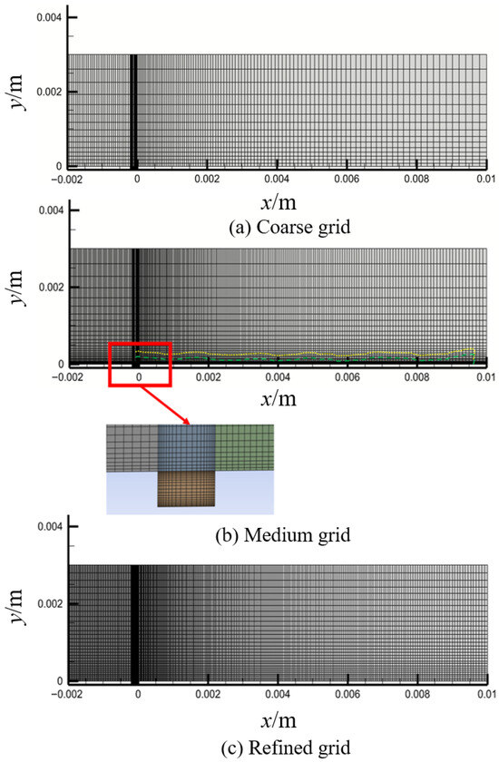
Figure 2.
Computational domain and mesh refinement: (a) coarse grid; (b) medium grid with a red frame indicating refinement at the injector; (c) adaptively refined grid at the interface region. Axes show coordinates in meters.
Refined grids were used to resolve broken ligaments and droplets, following the approach described in [69]. The mesh was also refined near the wall to capture the boundary layer, enabling an accurate prediction of the liquid film distribution. In critical near-wall regions, a structured computational mesh was employed, coupled with a laminar viscous model and an inflation growth rate of 1.2 to ensure accuracy and smooth grid transition.
Convergence for the simulations was typically achieved within 1000 iterations, determined by monitoring the solution residuals. The convergence criterion required a reduction in the energy equation residuals by three orders of magnitude [70], ensuring a stable and physically meaningful solution.
2.3. Mesh Independence Study
A mesh sensitivity analysis was conducted to evaluate the dependence of numerical results on spatial discretization (Figure 2). Three mesh resolutions were tested: coarse, medium, and refined, with increasing cell counts (Coarse: 2650 elements, 2889 nodes; Medium: 8800 elements, 9214 nodes; Refined: 11,700 elements, 12,214 nodes). The volume fraction of water at a representative monitored location was selected as the key comparative variable.
Figure 3 presents the time evolution of the water volume fraction for the three mesh resolutions. The coarse and medium meshes show negligible water volume until later time steps, while the refined mesh captures a significant volume fraction beginning earlier in the simulation. The substantial discrepancy between the refined mesh and the coarser meshes indicates that the phenomenon is highly sensitive to spatial resolution. The refined mesh resolves physical features—such as interface curvature and small-scale flow structures—that are numerically dissipated in the coarser meshes. While full mesh independence was not achieved within the tested resolutions, the medium mesh provides a compromise that captures the dominant physical trends observed in the refined case without the computational cost. The medium mesh was selected for all subsequent simulations for the following reasons:
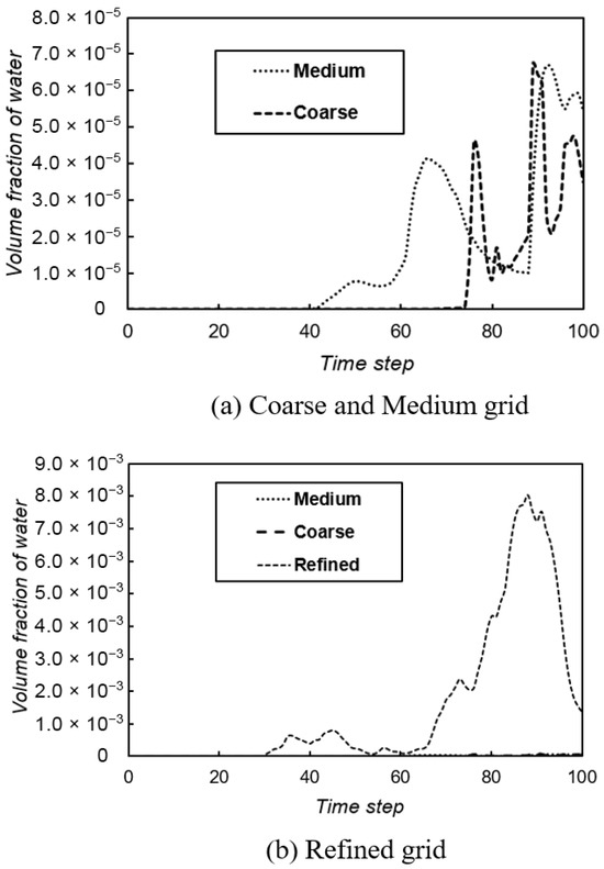
Figure 3.
Evolution of water volume fraction with time steps: (a) coarse and medium meshes; (b) refined mesh (separate scale).
- It exhibits trends similar to the coarse mesh but with better resolution of water transport onset.
- The refined mesh, although more detailed, requires prohibitively high computational time for the intended parameter studies.
- The primary focus of this study is on qualitative trends and relative comparisons under varying conditions, rather than absolute quantitative predictions of water volume fraction.
- The medium mesh balances numerical accuracy and computational feasibility within the scope of this work.
It is acknowledged that the simulations are not fully mesh-converged in the strict sense. Future work should involve higher-resolution simulations or adaptive mesh refinement to better capture the interfacially driven physics observed in the refined mesh case.
2.4. Boundary Conditions
The high-speed laminar flow was simulated using a coupled solver [71,72] and a transient formulation [73], with second-order upwind discretization for the governing equations [3]. The streamwise boundaries of the domain are defined as a periodic boundary condition pair. The jet injector uses a velocity inlet boundary condition. The top boundary is an adiabatic, slip wall, and the bottom wall is an isothermal, no-slip wall, except at the location of the jet. The working fluids are defined as an ideal gas for the air and liquid water for the coolant. The coolant jet enters the domain at the lower wall temperature.
This study comprised six computational simulations. Cases 1 through 5 investigated the necessary conditions for liquid film formation and stability, as well as the resulting overall system cooling effectiveness. Case 6 was specifically designed as a variant of Case 5 to isolate the effect of the numerical sound speed on boundary layer development. The computational domain is structured into four distinct blocks: the leading edge, the coolant-to-mainstream interface, the trailing edge, and the injector section. The setup modeled a single, short injection hole oriented at a 90° angle to the high-turbulence mainstream flow, incorporating an external flat plate. Appropriate boundary conditions were applied at the hole’s centerline, with the injector’s inlet defined 0.20 mm upstream and an outflow condition placed 0.10 mm downstream of the injection point.
The computational model for liquid film cooling on a flat plate, analyzed using both SPH and VOF methods, is shown in Figure 4. The liquid coolant is injected into the mainstream flow at the injection velocity v and injection angle θ specified in Table 1. The computational domain is 12 mm long and 3 mm high. A rectangular coolant jet slot, 0.2 mm wide and 0.1 mm high, is located such that its leading edge is 1.8 mm from the inlet and its trailing edge is 10.0 mm from the outlet. The domain’s streamwise length ensures full development of the liquid film on the lower wall, and its height prevents upper-wall reflections of the incident and jet-induced separation shock waves from compromising the lower wall’s cooling [74]. Periodic boundary conditions are applied at the inlet and outlet, while the flat plate is modeled as an isothermal wall with a constant temperature of 296 K.
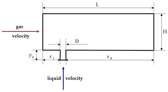
Figure 4.
Schematic of the mathematical model, illustrating the flow directions: red arrows represent hot air, and blue arrows represent cold coolant.

Table 1.
Operating parameters.
The applicability of the laminar flow model was verified by calculating the local Reynolds number at the extremity of the computational domain. For a characteristic streamwise length of
(the distance from the leading edge to the domain outlet) and under the core flow conditions (
,
, at
), the Reynolds number is
. This value remains well below the standard critical Reynolds number for boundary layer transition on a smooth flat plate (
), validating the laminar assumption for the present analysis.
The key geometric parameters of the computational domain and injection system, illustrated in Table 2, are defined as follows:
L: computational domain length;
H: computational domain height;
D: diameter of the injection hole;
: depth of the injection hole;
,
: distances from the center of the hole to the left and right boundaries, respectively.
Table 2.
Geometric Parameters of the Computational Domain and Injection System.
Table 2.
Geometric Parameters of the Computational Domain and Injection System.
| Parameters | Values | Dimensions |
|---|---|---|
| L | 12 | (mm) |
| H | 3 | (mm) |
| D | 0.2 | (mm) |
| 0.1 | (mm) | |
| 1.8 | (mm) | |
| 10 | (mm) | |
| θ | 90 | degree |
3. Results and Discussion
3.1. Comparison of the Laminar Model
A comparative analysis of the SPH and VOF methods was performed for the present laminar model. This comparison exercise was performed under identical boundary conditions to ensure a consistent basis for comparison. The assessment focused on key hydrodynamic and thermal parameters, namely film morphology, surface coverage, film thickness, and spatial variations in velocity and temperature. Comparisons were performed at three locations: immediate post-injection impact (x/D = 0), the mid-point development (x/D = 5), and the final flow establishment (x/D = 10). The results from both models establish the optimal method for predicting film cooling efficiency.
3.2. Film Morphology Analysis
To identify the parameters conducive to stable film formation, simulations were conducted across a range of flow conditions. The resulting morphologies are categorized as follows: Case 1 (Figure 5a) exhibits a stable, developed flow with a localized end effect. In contrast, Cases 2, 3, and 5 (Figure 5b) are characterized by a highly unstable, wavy flow. Case 4 (Figure 6c) demonstrates a smooth transition to a stable and well-developed state. The most critical regime is observed in Case 6 (Figure 5c), where jet lift-off occurs. In this condition, the liquid coolant completely detaches from the flat plate, exposing it directly to the high-temperature mainstream gas.
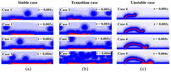
Figure 5.
Classification of film morphology from SPH simulations into stable, transitional, and unstable regimes: (a) stable, developed flow with a localized end effect; (b) highly unstable, wavy flow; (c) jet lift-off.
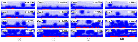
Figure 6.
SPH simulation results showing liquid film evolution over time. (a) Case 2 and (b) Case 3 represent stable film regimes. (c) Case 4 and (d) Case 5 represent transitional regimes leading to film break-up.
3.3. Temporal Film Coverage Variation
This subsection analyzes the evolution of liquid film length over time, presenting a direct comparison between the SPH and VOF methods, as illustrated in Figure 7. This study’s comparison focuses on quantifying the relative error for two key parameters: film thickness and coverage length. The analysis reveals specific error magnitudes across different temporal cases; for instance, at t = 0.0025 s, the relative errors for coverage length and thickness are 13.85% and 11.11%, respectively. Similarly, at t = 0.001 s, these errors measure 10.0% and 4.0%, and at t = 0.0015 s, they are 3.23% and 8.0%. The conducted error analysis is crucial for model comparison and directly supports the accurate prediction of optimal flow conditions. By precisely quantifying the discrepancies between the SPH and VOF models, this comparison identifies the parameter ranges where the simulations are most reliable. Ultimately, this predictive capability is essential for determining the flow conditions that yield the most effective cooling efficiency, thereby directly linking numerical model accuracy to the practical performance outcome. The relative errors for film thickness and film length are calculated using Equations (6) and (7), respectively. In the VOF method, an unequal flow volume was observed at the injection point and propagated downstream. This phenomenon is due to low coolant flow momentum (i.e., very low velocities) or a low mass flow rate. In contrast, this issue does not occur in the SPH model, which benefits from inherently lower numerical dissipation.
where
is the relative error in the film thickness,
is the relative error in the film coverage,
is the true thickness,
is the calculated thickness,
is the true coverage, and
is the calculated coverage.


Figure 7.
Comparison of liquid film morphology between SPH (left column) and FVM+VOF (right column) methods at different times for three cases. (a): Case 1 at 0.001 s and 0.0015 s; (b): Case 2 at 0.001 s and 0.0015 s; (c): Case 3 at 0.0015 s and 0.0025 s.
Figure 7.
Comparison of liquid film morphology between SPH (left column) and FVM+VOF (right column) methods at different times for three cases. (a): Case 1 at 0.001 s and 0.0015 s; (b): Case 2 at 0.001 s and 0.0015 s; (c): Case 3 at 0.0015 s and 0.0025 s.


3.4. Film Thickness: Stability, Chaos, and Recovery
The evolution of the liquid film thickness reveals distinct hydrodynamic regimes governed by the competition between inertial spreading, interfacial shear, and flow development. Both models capture the expected initial thinning due to downstream acceleration and spreading. However, their predictions diverge significantly in both magnitude and downstream development, highlighting model-dependent representations of interfacial stability and momentum transfer. In the VOF simulation, the film exhibits a non-monotonic thickness profile: after an initial decrease, it thickens again farther downstream (Figure 8a). This recovery suggests the onset of an adverse pressure gradient or reduced wall shear, allowing the film to re-accumulate—a behavior consistent with boundary-layer separation or a transition in local flow confinement.
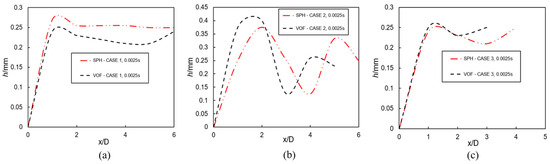
Figure 8.
Comparison of liquid film thickness (h/mm) profiles from VOF and SPH models at 0.0025 s, plotted against normalized downstream distance (x/D). (a) Case 1; (b) Case 2; (c) Case 3.
Conversely, the SPH model predicts a consistently thicker film that stabilizes rapidly within a short downstream distance. This rapid stabilization implies an early balance between inertia, viscous shear, and surface tension, leading to a quasi-steady developed film over most of the domain. The absence of re-thickening in SPH suggests a different representation of shear stress and pressure distribution near the interface.
The systematic over-prediction of film thickness by SPH, compared to VOF, points to fundamental differences in how each method resolves interfacial stresses and mass conservation. SPH’s particle-based formulation, with its inherent smoothing, may dampen interfacial instabilities and reduce effective shear, thereby maintaining a thicker, smoother film. VOF, with its sharper interface capture, appears more sensitive to shear-induced thinning and subsequent flow deceleration or separation effects.
These discrepancies underscore how core numerical approaches—namely, interface sharpening in VOF versus momentum/volume smoothing in SPH—qualitatively influence the predicted film dynamics, particularly in regions where the flow approaches stability thresholds.
The interfacial response to flow development differs markedly between the two numerical approaches at this early stage (t = 0.0025 s, Figure 8b).
- (a)
- The VOF simulation yields a film profile with a single, dominant disturbance, suggesting a stable or quickly damped interfacial response.
- (b)
- In contrast, the SPH result at the same instant shows a profile with multiple wave peaks and troughs, indicating the presence of stronger or more numerous initial interfacial perturbations. This contrast at t = 0.0025 s suggests that the initial numerical treatment of interfacial curvature, stress, and perturbations differs fundamentally between the methods. The SPH formulation appears more susceptible to generating or sustaining short-wavelength interfacial disturbances early in the simulation, while VOF produces a smoother initial profile that may be more numerically damped.
In both models, the film undergoes a cycle of downstream thinning followed by recovery (Figure 8c), consistent with a balance between inertial spreading and viscous–capillary resistance. However, the development length and severity of thinning differ markedly.
VOF predicts a more extended and gradual development region with a shallower thickness minimum, reflecting the higher numerical diffusion characteristic of many interface-capturing schemes, which can smear sharp gradients and dampen local extremes.
SPH, in contrast, resolves a sharper, more localized minimum and a more abrupt recovery. This is consistent with SPH’s ability to sharply resolve interfaces and local curvatures with minimal numerical dissipation, allowing it to capture stronger local thinning and recoil effects [3].
Over an overlapping streamwise range, both models capture the same physical trend—supporting the general reliability of the simulations—but the amplitude and sharpness of the minimum are governed by the inherent diffusion (VOF) or sharpness (SPH) of each method’s interface treatment.
The wave formation dynamics, as depicted in Figure 9, are captured qualitatively by both models, confirming the underlying physical instability. Each simulation resolves the canonical sequence of a downstream-propagating disturbance: inertial accumulation forms a crest, which subsequently relaxes and stretches the film to produce a pronounced trough. While the models agree on the spatial phasing of this crest–trough structure, they differ in wave amplitude. The SPH model consistently predicts a higher crest, attributable to its lower numerical dissipation and sharper interface resolution. In contrast, the VOF solution exhibits a damped crest height due to inherent numerical diffusion, which artificially smooths the interfacial curvature [75]. Notably, both models converge on the same trough depth and location, indicating that the thinning mechanism—driven by inertial stretching downstream of the crest—is physically robust and less sensitive to numerical methodology. The strong agreement in the wave’s spatial evolution and trough characteristics provides confidence that the simulated instability is physical, not numerical. The remaining discrepancy in crest magnitude serves as a direct measure of each method’s interfacial sharpness and damping characteristics.
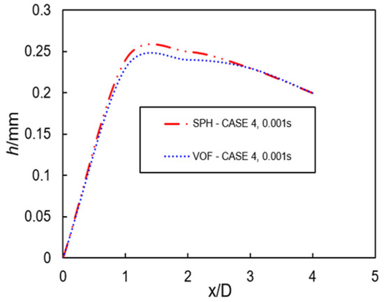
Figure 9.
Variation in Liquid Film Thickness (h/mm) along the normalized downstream distance (x/D) for Case 4 at 0.001 s: Comparison of VOF and SPH Models.
The temporal evolution of liquid film thickness captures a distinct physical progression from stability through a violent instability to partial recovery. Initially, the film exhibits a damped, symmetric disturbance—a hallmark of a stable, smooth flow regime. This is followed by the emergence of a severe wave-breaking event, characterized by extreme local thinning indicative of interfacial rupture. Subsequently, the flow partially re-stabilizes, settling into a thinner, yet still perturbed, equilibrium state. This chronology is corroborated by both models, which qualitatively agree on each flow regime. Quantitatively, the SPH model consistently predicts a thicker film in the stable phase, a discrepancy attributable to its lower numerical diffusion. During the wave-breaking instability, both methods resolve the same catastrophic thinning, confirming the event as a physical, rather than numerical, phenomenon. The post-break recovery towards a thinner equilibrium suggests a permanent redistribution of momentum and a change in the local force balance following the extreme event. The liquid film thickness (h) data for Case 2 (timestep = 0.002 s) are presented in Table 3.
Table 3.
Film Thickness (h/mm) during the Wave Breaking at t = 0.002 s.
The wave-breaking event exhibits a pronounced crest-trough-overshoot sequence, characteristic of a violent interfacial instability. A large-amplitude crest forms, signifying significant local fluid accumulation, which is immediately followed by extreme film thinning downstream—a signature of inertial stretching approaching the breakup limit. The subsequent oscillatory recovery, marked by a secondary peak, reflects the chaotic relaxation of the interface as it seeks a new equilibrium.
Following this event, the flow partially re-stabilizes. The film adopts a progressively thinning profile along the streamwise direction, eventually reaching a steady, attenuated state. This final configuration represents a new force balance established after the dissipation of energy from the prior instability. The liquid film thickness (h) data for Case 1 (timestep = 0.0025 s) are presented in Table 4.
Table 4.
Film Thickness (h/mm) during Re-stabilization at t = 0.0025 s.
Following the wave-breaking event, the film re-stabilizes into a permanently thinner and more uniform state. This new equilibrium results from the dissipation of energy injected during the violent instability, which redistributes momentum and alters the local balance between inertial, viscous, and capillary forces. Residual mild undulations persist, confirming that the flow has not returned to its original laminar condition but has transitioned to a lower-energy, stable-wavy regime.
The overall progression—from initial disturbance to wave growth, breakup, and eventual stabilization—is captured by both models and aligns with a shear-driven interfacial instability, such as a Kelvin–Helmholtz mode [74]. While the models agree qualitatively on this sequence, quantitative differences emerge in the severity and phasing of events. The VOF simulation, with its inherent numerical diffusion, predicts a slightly earlier and more damped wave breakdown. In contrast, the SPH method, which minimizes artificial smoothing, resolves a sharper crest–trough structure and a more pronounced post-breakup oscillation, reflecting a higher-fidelity representation of interfacial physics during violent stretching and relaxation.
These discrepancies highlight how numerical diffusion directly modulates the apparent intensity and temporal development of the instability, yet both approaches confirm the central physical narrative: a finite perturbation can trigger a catastrophic transition to wave breaking, followed by irreversible thinning and stabilization.
The SPH simulations (Figure 10a) resolve three fundamental flow regimes dictated by the balance between shear-driven destabilization and viscous-capillary restoration. A chaotic inertial regime emerges under high gas shear, characterized by large-amplitude, non-periodic waves where disturbances are generated faster than interfacial tension can stabilize them. This indicates a flow dominated by kinetic energy and far from equilibrium. In contrast, a stabilizing viscous regime develops when increased liquid inertia or favorable conditions enhance damping. Here, the film exhibits a monotonic downstream thinning and attenuation of waves, signifying a transition toward a laminar, shear-dominated equilibrium as viscous forces smooth the interface. A third, stable wavy regime is also identified, where the film maintains small, coherent fluctuations in a statistically steady, fully developed state. This regime represents a saturated equilibrium between disturbance growth and damping. In all cases, a downstream thickening is observed and attributed to a boundary-induced pooling effect, confirming that the core flow physics are distinct from domain artifacts. The primary driver separating these regimes is the relative magnitude of shear forcing versus the stabilizing effects of viscosity and surface tension. High shear promotes wave growth and chaos, while conditions favoring damping lead to stabilization and laminarization [3].
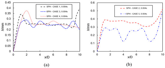
Figure 10.
Liquid film thickness (h/mm) versus normalized downstream distance (x/D) at 0.004 s: comparison of SPH simulation results for Cases 1–5. (a) Cases 1, 3, and 4, exhibiting a transition to a laminar, shear-dominated equilibrium; (b) Cases 2 and 5, characterized by a laminar equilibrium regime followed by wave growth and catastrophic thinning.
Figure 10b reveals two divergent flow regimes dictated by the competition between destabilizing shear and stabilizing forces. The first is a laminar equilibrium regime, characterized by a uniform film thickness indicative of a near-perfect balance between inertia, viscous stress, and surface tension. This stable, quasi-parallel flow results from conditions that suppress disturbance growth, such as high liquid viscosity and low gas shear. The second is a coherent wave-breaking regime, defined by periodic, severe troughs where the film thins to near-breakup thickness. This regular cycle of wave growth and catastrophic thinning demonstrates a powerful, inherent hydrodynamic instability with a well-defined wavelength. The instability is driven by high shear and inertial forcing, which inject energy into the interface faster than capillary and viscous forces can restore stability [74]. Both regimes exhibit downstream thickening attributable to boundary-induced pooling, confirming this as a domain artifact rather than a physical feature of the core flow. The stark contrast between the regimes underscores that flow stability is governed by the relative magnitude of shear-driven energy input versus dissipative and restorative mechanisms.
3.5. Analysis of Velocity Variations
The development of the liquid film is governed by its disruptive effect on the high-speed gas stream, a mechanism directly probed by analyzing mainstream velocity evolution. During the critical initial transient following injection, a clear divergence emerges between flow regimes (Figure 11a). Conditions that promote a stable, well-attached film (e.g., lower coolant flow rate, favorable wettability) result in minimal gas flow disruption. The mainstream velocity exhibits only a slight, transient dip as momentum is transferred during film establishment, followed by a rapid recovery to a high equilibrium value. This indicates a streamlined gas-liquid interface with efficient phase coupling and low turbulence generation. In contrast, conditions leading to a more disruptive injection cause sustained momentum loss in the gas phase. The mainstream velocity fails to recover, remaining attenuated as energy is continuously dissipated through interfacial instability and increased shear. This establishes a direct causal link: film stability controls gas flow modulation, where a smooth interface minimizes blockage while an unstable interface acts as a persistent source of momentum loss and turbulence.
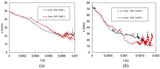
Figure 11.
Comparison of mainstream velocity (m/s) at the injection point using the VOF model. (a) Cases 1 and 2 at 0.001 s; (b) Cases 4 and 5 at 0.0019 s.
In stark contrast, the second flow regime exhibits a highly disruptive interaction. Here, the mainstream velocity undergoes severe and continuous attenuation, indicative of massive momentum transfer from the gas to the liquid phase. This behavior is characteristic of an injection process that violently disrupts the gas stream. The underlying physics involve significant flow blockage and boundary layer separation. The higher-momentum coolant injection generates large interfacial waves and likely prompts droplet entrainment, creating a thick, unstable film that acts as a substantial obstacle. This forces the gas flow to separate, forming a low-momentum recirculation zone or wake above the injection point. The consequent destruction of the protective gaseous boundary layer signifies an inefficient cooling configuration, where the liquid film is immediately susceptible to breakup due to poor adhesion and excessive interfacial shear.
The initial shear-driven instability at the point of injection dictates subsequent film development [3], as shown in the mainstream velocity transients (Figure 11b). Both regimes exhibit large-amplitude oscillations characteristic of a Kelvin-Helmholtz-type instability [74], where the high-velocity gas shearing over the liquid jet triggers vortex shedding and rapid wave breakdown [3]. The key distinction lies in the mean momentum of the injected liquid. A high-momentum injection penetrates further into the gas stream, resulting in violent, high-energy interactions centered around an elevated mean velocity. This suggests a greater potential to establish a persistent, attached film downstream. Conversely, a low-momentum injection is rapidly sheared and accelerated by the gas, producing oscillations around a lower mean velocity. This indicates a higher susceptibility to complete disruption, increasing the likelihood of downstream film breakup and dry-out. The intense fluctuations confirm that the flow at this early stage is dominated by transient shear instability, not by a quasi-steady balance. The mean injection momentum thus serves as a primary predictor of whether the interaction will lead to film establishment or prompt disintegration.
Downstream propagation reveals a lasting signature of the initial injection disturbance (Figure 12). While both flows exhibit recovery from the near-injection transients, a significant performance divergence remains. The regime characterized by a stable, attached film facilitates the rapid re-establishment of a high-momentum gas boundary layer. This efficient recovery indicates minimal flow blockage and low interfacial resistance, allowing the gas stream to quickly overcome the initial disruption. In contrast, the regime originating from a disruptive injection exhibits a persistent momentum deficit. The slower and more erratic velocity recovery suggests that the large-scale separation and recirculation generated at injection convect downstream, sustaining a thick, turbulent boundary layer. This confirms that an unstable liquid film acts as a continuing source of flow obstruction, impeding boundary layer reattachment and efficient momentum transfer far beyond the immediate injection site. The downstream state is thus a direct consequence of near-wall interface morphology: a smooth film promotes boundary layer recovery, while a disturbed film propagates a wake-like disturbance that degrades gas flow efficiency.
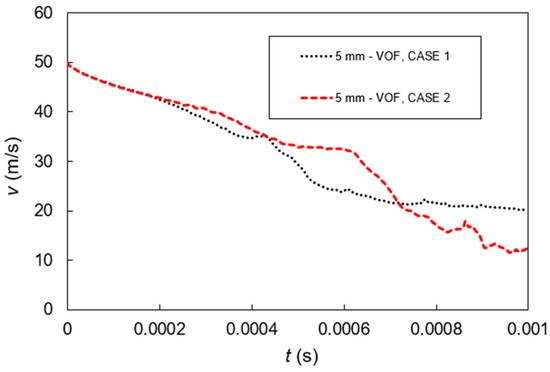
Figure 12.
Mainstream velocity (m/s) variations at the mid-point along the normalized downstream distance (x/D) at 0.001 s: Comparison of VOF Models (cases 1 and 2).
At the domain outlet, the flow exhibits the long-term consequences of initial film stability (Figure 13a). For regimes beginning with stable injection, the primary feature is the classic development of a laminar or transitional boundary layer [74] over the smooth film, as evidenced by a monotonic velocity decay due to viscous growth. This confirms effective, low-loss momentum transport across the entire plate. For regimes originating from disruptive injection, the severe near-field separation and turbulence have largely dissipated by the outlet. The flow has reattached and is developing a new, thicker boundary layer. While this results in partial recovery of the mean velocity profile, the process incurs higher viscous losses compared to the stable case. In contrast, regimes characterized by sustained interfacial waves exhibit a fundamentally different downstream state (Figure 13b). The convective passage of waves continuously perturbs the gas boundary layer, preventing it from achieving a steady, developed profile. Each wave crest acts as a recurring local obstruction, maintaining flow unsteadiness and inhibiting acceleration far downstream. This demonstrates that while gross flow separation can recover, persistent interfacial instability imposes a continuous momentum penalty that propagates throughout the domain.
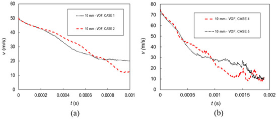
Figure 13.
Comparison of mainstream velocity (m/s) at the end of the plate using the VOF model. (a) Cases 1 and 2 at 0.001 s; (b) Cases 4 and 5 at 0.0019 s.
3.6. Analysis of Temperature Variations
The initial thermal response is governed by the competing fluxes of convective heating from the hot gas and convective/evaporative cooling from the liquid film (Figure 14). A clear performance hierarchy emerges, directly correlated with the coolant flow rate and the consequent stability of the near-injection film. Cases with higher injection momentum and flow rate establish a robust, persistent liquid film that effectively blankets the surface. This stable film provides continuous cooling through sensible heat absorption and, critically, enables efficient evaporative heat transfer due to sustained liquid-gas contact. The result is a rapid, deep temperature drop with minimal fluctuations, indicating a dominant cooling flux. In contrast, lower flow rates produce a weak, intermittent film that is readily entrained by the gas stream. This leads to insufficient thermal mass for heat absorption and periodic exposure of the surface to hot gas. The cooling flux is thus overcome by the heating flux, resulting in a shallower temperature reduction with greater unsteadiness, signaling inadequate thermal protection. The terminal temperature at the injection point therefore serves as a direct indicator of the local cooling efficiency, which is fundamentally controlled by the liquid film’s ability to maintain coverage and promote phase-change heat transfer.
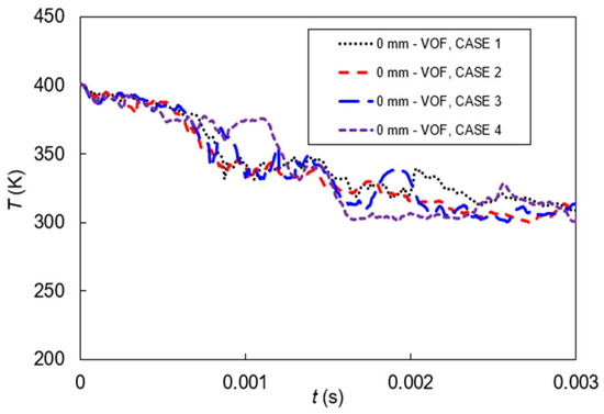
Figure 14.
Temperature Variation along the normalized distance (x/D) at the Injection Point at t = 0.003 s (Cases 1, 2, 3, 4): Comparison of VOF Models.
Downstream thermal performance bifurcates into two distinct regimes dictated by interfacial stability (Figure 15). Successful cooling is achieved when sufficient injection momentum establishes a continuous liquid film that adheres and propagates. This film provides effective thermal protection through convective cooling and, critically, evaporative heat transfer, balancing the gas-side heating flux and maintaining a low surface temperature. In contrast, insufficient injection momentum leads to immediate film disintegration via shear-driven entrainment. The liquid is atomized and carried away, causing dry-out upstream of the measurement location. This exposes the surface directly to the hot gas, resulting in location thermal equilibrium at a significantly elevated temperature.
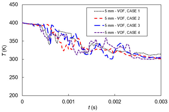
Figure 15.
Temperature Variation Mid-Point along the normalized distance (x/D) at t = 0.003 s (Cases 1, 2, 3, 4): Comparison of VOF Models.
The mid-point temperature thus serves as a definitive marker of the film’s hydrodynamic integrity. A low temperature confirms the presence of a persistent, cooling-capable film, while a high temperature signals catastrophic dry-out due to inadequate momentum to resist interfacial shear.
The final thermal state at the plate outlet (Figure 16) confirms a direct relationship between liquid film integrity and cooling efficacy. The performance gradient correlates precisely with the coolant’s capacity to establish and maintain a continuous protective layer against the hot gas stream. Optimal cooling is achieved when sufficient injection momentum creates a thick, stable film that adheres and propagates rapidly. This film provides effective insulation and, due to its greater thermal mass and capacity for evaporative cooling, establishes a dominant heat sink, resulting in a sharp, sustained temperature drop. Conversely, lower injection momentum leads to progressive degradation. The film becomes thinner, intermittent, and susceptible to shear-driven breakdown. This results in partial or complete dry-out, where the surface is periodically or wholly exposed to convective heating, leading to a diminished and delayed cooling response. The weakest injection produces immediate film disintegration, yielding negligible thermal protection. The terminal temperature profile is therefore a direct signature of the film’s hydrodynamic stability. The cooling hierarchy demonstrates that the critical threshold for effective thermal management is the injection condition required to overcome interfacial shear and prevent dry-out.
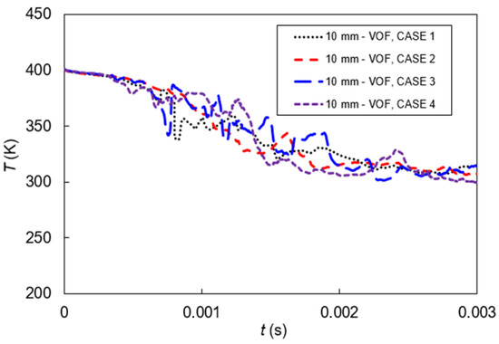
Figure 16.
Temperature Variation along the normalized distance (x/D) at the End of the isothermal plate for t = 0.003 s (Cases 1, 2, 3, 4): Comparison of VOF Models.
The numerical results demonstrate qualitative agreement with established experimental trends for liquid film cooling. Key phenomena such as film thinning, lateral spread, and the onset of liquid film lift-off are consistent with observations in the literature [69]. Furthermore, the simulations successfully capture the interfacial dynamics driven by shear: Kelvin-Helmholtz instability generates waves at the air-liquid interface, which amplify downstream and lead to film rupture and droplet formation.
4. Conclusions
This study has successfully developed and compared a dual-methodology numerical framework, combining SPH and VOF methods, to investigate the complex, transient behavior of liquid coolant films under high-shear gas flow. This research provides a comprehensive, physics-based model that directly links hydrodynamic film stability to surface thermal management efficacy, moving beyond mere observation to establish predictive principles.
This investigation yielded three primary scientific insights into film behavior. First, film stability is not a binary state but a lifecycle sensitive to the precise balance of inertial, viscous, and capillary forces, with sonic speed in the gas stream emerging as a dominant control parameter. Second, the initial injection conditions—specifically, the achievement of a critical coolant momentum threshold—dictate the ultimate thermal performance by determining early-stage flow attachment or separation. Third, a robust cross-comparison between the SPH and VOF models confirmed the physical reality of key simulated dynamics, such as acceleration-thinning and capillary recovery. This methodological comparison also highlighted SPH’s superior fidelity in resolving fine-scale interfacial instabilities, a critical capability for simulating violent breakup processes.
More broadly, this work offers two key contributions to the field of active cooling simulation. It establishes that overall cooling effectiveness is governed by initial flow conditions, underscoring the paramount importance of stable injection design. Furthermore, it identifies the rapid temperature drop associated with a stable film as a key diagnostic metric for optimal performance, providing a clear, causal link between hydrodynamic stability and thermal outcome.
Future Work
This comparative framework and its insights pave the way for several important research directions:
- The observed crest and trough dynamics—including wavelength, amplitude, and growth/decay rates—provide a clear, quantitative signature for future theoretical linear stability analysis. This will allow for the derivation of instability thresholds and growth rates directly from first principles, deepening the theoretical foundation of our numerical observations.
- Future studies will implement a systematic parametric sweep of key governing dimensionless numbers, particularly the Mach and Reynolds numbers, to construct a detailed flow regime map. This map will explicitly link simulation outcomes to classical laminar-wavy-transition flow theory, enabling predictive design for different operating conditions.
- Building on the established link between hydrodynamics and cooling, this work provides a foundation for optimizing injector geometry to reliably achieve and maintain the stable film regime identified here.
- The framework is also extensible to exploring more complex fluids (e.g., non-Newtonian coolants), multi-jet interactions, and the full integration of conjugate heat transfer models to further close the loop between flow prediction and thermal system design.
Author Contributions
E.M.U.: conceptualization, methodology, software, investigation, formal analysis, data curation, visualization, writing—original draft preparation, writing—review and editing. H.L.: conceptualization, software, methodology, investigation, writing—review, and editing. X.Y.: methodology, software, resources, supervision, project administration, funding acquisition, writing—review, and editing. D.A.U.: software, investigation, writing—review, and editing. N.K.: software, investigation, writing—review, and editing. All authors have read and agreed to the published version of the manuscript.
Funding
This work was supported by the National Natural Science Foundation of China (Grant No. 12172049) and the National Key Laboratory of Aircraft Configuration Design Foundation (Grant No. ZYTS-202405).
Data Availability Statement
The datasets presented in this study are available within this article. Any additional data required to support the findings are available from the corresponding author upon reasonable request.
Conflicts of Interest
Each author has declared no conflicts of interest. Additionally, the funders had no role in this study’s design, data collection, analysis, data interpretation, manuscript writing, or the decision to publish this work.
Nomenclature
| c | Sonic speed (unit: m/s) |
| Specific heat (unit: J/(kg.K)) | |
| ρ | Density (unit: kg/m3) |
| h | Film thickness (unit: mm)/smoothing length |
| k | Thermal conductivity (unit: W/(m.K)) |
| p | Pressure (unit: Pa) |
| t | Time (unit: s) |
| q | Heat flux vector |
| S | Stress tensor |
| T | Temperature (unit: K) |
| μ | Viscosity (unit: Pa.s) |
| v | Velocity (unit: m/s) |
| x/D | Downstream distance |
| D | Coolant jet slot diameter (unit: mm) |
| DR | Density ratio |
| ds | Initial particle spacing |
| H | Height of the computational domain |
| L/D | Length-to-diameter ratio |
| θ | Injection angle (unit: degrees) |
| Subscript | |
| b | boundary/computational domain |
| E | true thickness/coverage |
| S | calculated thickness/coverage |
| i | fixed particle |
| J | neighbouring particle |
| RC | relative error in the film coverage |
| RT | relative error in the film thickness |
| x, y, l | Source terms |
| Abbreviation | |
| CFD | Computational Fluid Dynamics |
| FSI | Fluid Structure Interaction |
| FSTI | Free-Stream Turbulence Intensity |
| FVM | Finite Volume Method |
| SPH | Smoothed Particle Hydrodynamics |
| VOF | Volume of Fluid |
| TIT | Turbine inlet temperature |
References
- Peters, A.B.; Zhang, D.; Chen, S.; Ott, C.; Oses, C.; Curtarolo, S.; McCue, I.; Pollock, T.M.; Prameela, S.E. Materials design for hypersonics. Nat. Commun. 2024, 15, 3328. [Google Scholar] [CrossRef]
- Liu, J.; Xu, M.; Guo, W.; Xi, W.; Liu, C.; Sunden, B. Flow and Heat Transfer Mechanism of a Regenerative Cooling Channel Mounted with Pin-Fins Using Supercritical CO2 as Coolant. Int. J. Therm. Sci. 2025, 208, 109425. [Google Scholar] [CrossRef]
- Umana, E.M.; Yang, X. Review of Film Cooling Techniques for Aerospace Vehicles. Energies 2025, 18, 3085. [Google Scholar] [CrossRef]
- Shine, S.R.; Shri Nidhi, S. Review on film cooling of liquid rocket engines. J. Propuls. Power Res. 2018, 7, 1–18. [Google Scholar] [CrossRef]
- Montis, M.; Ciorciari, R.; Salvadori, S.; Carnevale, M.; Niehuis, R. Numerical prediction of cooling losses in a high-pressure gas turbine airfoil. Proc. Inst. Mech. Eng. Part A J. Power Energy 2014, 228, 903–923. [Google Scholar] [CrossRef]
- Ba, W.; Li, X.; Ren, X.; Gu, C. Aero-thermal coupled through-flow method for cooled turbines with new cooling model. Proc. Inst. Mech. Eng. Part A J. Power Energy 2018, 232, 254–265. [Google Scholar] [CrossRef]
- Heufer, K.A.; Olivier, H. Experimental and numerical study of cooling gas injection in laminar supersonic flow. AIAA J. 2008, 46, 2741–2751. [Google Scholar] [CrossRef]
- Juhany, K.A.; Hunt, M.L.; Sivo, J.M. Influence of injectant Mach number and temperature on supersonic film cooling. J. Thermophys. Heat Transf. 1994, 8, 59–67. [Google Scholar] [CrossRef]
- Zhou, C.; Wang, Z.; Hou, T. Heat transfer analysis of thermal protection structures for hypersonic vehicles. IOP Conf. Ser. Mater. Sci. Eng. 2017, 269, 12020. [Google Scholar] [CrossRef]
- Shine, S.R.; Kumar, S.S.; Suresh, B.N. Internal wall-jet film cooling with compound angle cylindrical holes. Energy Convers. Manag. 2013, 68, 54–62. [Google Scholar] [CrossRef]
- Papell, S.S. Effect on Gaseous Film Cooling Injection Through Angled Slots and Normal Holes; NASA TN-D-299; National Aeronautics and Space Administration (NASA): Washington, DC, USA, 1960. [Google Scholar]
- Hartnett, J.P.; Birkebak, R.C.; Eckert, E.R.G. Velocity distributions, temperature distributions, effectiveness, and heat transfer for air injected through a tangential slot into a turbulent boundary layer. ASME J. Heat Transf. 1961, 83, 293–305. [Google Scholar] [CrossRef]
- Seban, R.A.; Back, L.H. Effectiveness and heat transfer for a turbulent boundary layer with tangential Injection and variable free-stream velocity. ASME J. Heat Transf. 1962, 84, 235–242. [Google Scholar] [CrossRef]
- Burns, W.K.; Stollery, J.L. The Influence of foreign gas injection and slot geometry on film cooling effectiveness. Int. J. Heat Mass Transf. 1969, 12, 935–995. [Google Scholar] [CrossRef]
- Goldstein, R.J.; Eckert, R.G.; Bljrgciraf, F. Effects of hole geometry and density on three-dimensional film cooling. Int. J. Heat Mass Transf. 1974, 17, 595–607. [Google Scholar] [CrossRef]
- Pedersen, D.R.; Eckert, E.R.G.; Goldstein, R.J. Film cooling with large density differences between the mainstream and the secondary fluid measured by the heat-mass transfer analogy. ASME J. Heat Transf. 1977, 99, 620–627. [Google Scholar] [CrossRef]
- Wright, L.M.; McClain, S.T.; Clemenson, M.D. Effect of density ratio on flat plate film cooling with shaped holes using PSP. ASME J. Turbomach. 2011, 133, 041011. [Google Scholar] [CrossRef]
- Cho, H.; Rhee, D.H.; Kim, B.G. Enhancement of film cooling performance using a shaped film cooling hole with compound angle injection. JSME 2001, 44, 99–109. [Google Scholar] [CrossRef]
- Haven, B.A.; Kurosaka, M. Kidney and anti-kidney vortices in crossflow jets. ASME J. Fluid Mech. 1997, 352, 27–64. [Google Scholar] [CrossRef]
- Saumweber, C.; Schulz, A.; Wittig, S. Free-stream turbulence effects on film cooling with shaped holes. J. Turbomach. 2003, 125, 65–73. [Google Scholar] [CrossRef]
- Kuldeep, S.; Premachandran, B.; Ravi, M.R. Experimental assessment of film cooling performance of short cylindrical holes on a flat surface. J. Heat Mass Transf. 2016, 52, 2849–2862. [Google Scholar] [CrossRef]
- Dhungel, A.; Lu, Y.; Phillips, W.; Ekkad, S.V.; Heidmann, J. Film cooling from a row of holes supplemented with antivortex holes. J. Turbomach. 2009, 131, 021007. [Google Scholar] [CrossRef]
- Yiping, L.; Dhungel, A.; Ekkad, S.V.; Bunker, R.S. Film cooling measurements for cratered cylindrical inclined holes. ASME J. Turbomach. 2009, 131, 011005. [Google Scholar]
- Yiping, L.; Dhungel, A.; Ekkad, S.V.; Bunker, R.S. Effect of trench width and depth on film cooling from cylindrical holes embedded in trenches. ASME J. Turbomach. 2009, 131, 011003. [Google Scholar]
- Burd, S.; Kaszeta, R.W.; Simon, T. Measurements in film cooling flows: Hole L/D and turbulence intensity effects. ASME J. Turbomach. 1998, 120, 791–798. [Google Scholar] [CrossRef]
- Ligrani, P.M.; Bell, C.M. Film cooling subject to bulk flow pulsations: Effects of density ratio, hole length-to-diameter ratio, and pulsation frequency. Int. J. Heat Fluid Flow 2001, 44, 2005–2009. [Google Scholar] [CrossRef]
- Gritsch, M.; Colban, W.; Schär, H.; Döbbeling, K. Effect of hole geometry on the thermal performance of fan-shaped film cooling holes. J. Turbomach. 2005, 127, 718–725. [Google Scholar] [CrossRef]
- Wilfert, G.; Wolff, S. Influence of internal flow on film cooling effectiveness. J. Turbomach. 2000, 122, 327–333. [Google Scholar] [CrossRef]
- Hale, C.A.; Plesniak, M.W.; Ramadhyani, S. Film Cooling Effectiveness for Short Film Cooling Holes Fed by a Narrow Plenum. J. Turbomach. 2000, 122, 553–557. [Google Scholar] [CrossRef]
- Lutum, E.; Johnson, B.V. Influence of the hole length-to-diameter ratio on film cooling with cylindrical holes. ASME J. Turbomach. 1999, 121, 209–216. [Google Scholar] [CrossRef]
- Morrell, G. Investigation of Internal Film Cooling of a 1000-Pound-Thrust Liquid-Ammonia-Liquid-Oxygen Rocket-Engine Combustion Chamber; Technical Report; NACA RME51E04; NTRS: Washington, DC, USA, 1951; pp. 1–40. [Google Scholar]
- Kesselring, R.C.; Knight, R.M.; McFarland, B.L.; Gurnitz, R.N. Boundary Cooled Rocket Engines for Space Storable Propellants; Technical Report; Rocketdyne Report No. R-8766; NTRS: Washington, DC, USA, 1972; pp. 1–264. [Google Scholar]
- Shine, S.R.; Kumar, S.S.; Suresh, B.N. Influence of coolant injector configuration on film cooling effectiveness for gaseous and liquid film coolants. Heat Mass Transf. 2012, 48, 849–861. [Google Scholar] [CrossRef]
- Knuth, E.L. The Mechanics of Film Cooling. Ph.D. Thesis, California Institute of Technology, Pasadena, CA, USA, 1954; pp. 1–108. [Google Scholar]
- Zhang, H.W.; Tao, W.Q.; He, Y.L.; Zhang, W. Numerical study of liquid film cooling in a rocket combustion chamber. Int. J. Heat Mass Transf. 2006, 49, 349–358. [Google Scholar] [CrossRef]
- Yu, Y.C.; Schuff, R.Z.; Anderson, W.E. Liquid film cooling using swirl in rocket combustors. In Proceedings of the 40th AIAA/ASME/SAE/ASEE Joint Propulsion Conference and Exhibit, Paper No. AIAA 2004-3360. Fort Lauderdale, FL, USA, 11–14 July 2004. [Google Scholar]
- Zaitsev, D.; Kochkin, D.; Kabov, O. Dynamics of liquid film rupture under local heating. Int. J. Heat Mass Transf. 2022, 184, 122376. [Google Scholar] [CrossRef]
- Oron, A.; Davis, S.H.; Bankoff, S.G. Long-scale evolution of thin liquid films. Rev. Mod. Phys. 1997, 69, 931–980. [Google Scholar] [CrossRef]
- Liu, J.; Schneider, J.B.; Gollub, J.P. Three-dimensional instabilities of film flows. Phys. Fluids 1995, 7, 55–67. [Google Scholar] [CrossRef]
- Pshenichnikov, A.F.; Tokmenina, G.A. Deformation of the free surface of a liquid by thermocapillary motion. Fluid Dyn. 1983, 18, 463–465. [Google Scholar] [CrossRef]
- Burelbach, J.P.; Bankoff, S.G.; Davis, S.H. Steady thermocapillary flows of thin liquid layers. II. Experiment. Phys. Fluids A Fluid Dyn. 1990, 2, 322–333. [Google Scholar] [CrossRef]
- Orell, A.; Bankoff, S.G. Formation of a dry spot in a horizontal liquid film heated from below. Int. J. Heat Mass Transf. 1971, 14, 1835–1842. [Google Scholar] [CrossRef]
- Kabov, O.A. Heat transfer from a small heater to a falling liquid film. Heat Transf. Res. 1996, 27, 221–226. [Google Scholar]
- Kabov, O.A. Breakdown of a liquid film flowing over the surface with a local heat source. Thermophys. Aeromech 2000, 7, 513–520. [Google Scholar]
- Bezuglyi, B.A.; Ivanova, N.A.; Zueva, A.Y. Laser–induced thermocapillary deformation of a thin liquid layer. J. Appl. Mech. Tech. Phys. 2001, 42, 493–496. [Google Scholar] [CrossRef]
- Ajaev, V.S.; Kabov, O.A. Heat and mass transfer near contact lines on heated surfaces. Int. J. Heat Mass Transf. 2017, 108, 918–932. [Google Scholar] [CrossRef]
- Kabov, O.A.; Zaitsev, D.V.; Kirichenko, D.P.; Ajaev, V.S. Interaction of levitating microdroplets with moist air flow in the contact line region. Nanoscale Microscale Thermophys. Eng. 2017, 21, 60–69. [Google Scholar] [CrossRef]
- Ajaev, V.S. Instability and rupture of thin liquid films on solid substrates. Interfac. Phenom. Heat Transf. 2013, 1, 81–92. [Google Scholar] [CrossRef]
- Zaitsev, D.V.; Kabov, O.A. An experimental modeling of gravity effect on rupture of a locally heated liquid film. Microgravity Sci. Technol. 2007, 19, 174–177. [Google Scholar] [CrossRef]
- Chhokar, C.; Ebadi, M.; Bahrami, M. The Total Heat Transfer Rate in the Evaporating Thin Film: A New Analytical Solution. Int. Commun. Heat Mass Transf. 2025, 162, 108653. [Google Scholar] [CrossRef]
- Wang, H.; Garimella, S.V.; Murthy, J.Y. Characteristics of an Evaporating Thin Film in a Microchannel. Int. J. Heat Mass Transf. 2007, 50, 3933–3942. [Google Scholar] [CrossRef]
- Potash, M.; Wayner, P.C. Evaporation from a Two-Dimensional Extended Meniscus. Int. J. Heat Mass Transf. 1972, 15, 1851–1863. [Google Scholar] [CrossRef]
- Wayner, P.C.; Kao, Y.K.; LaCroix, L.V. The Interline Heat-Transfer Coefficient of an Evaporating Wetting Film. Int. J. Heat Mass Transf. 1976, 19, 487–492. [Google Scholar] [CrossRef]
- Schrage, R.W. A Theoretical Study of Interphase Mass Transfer; Columbia University Press: New York, NY, USA, 1953. [Google Scholar] [CrossRef]
- Schonberg, J.A.; Wayner, P.C. An Analytical Solution for the Integral Contact Line Evaporative Heat Sink. J. Thermophys. Heat Transf. 1992, 6, 128–134. [Google Scholar] [CrossRef]
- DasGupta, S.; Schonberg, J.A.; Wayner, P.C. Investigation of an Evaporating Extended Meniscus Based on the Augmented Young–Laplace Equation. J. Heat Transf. 1993, 115, 201–208. [Google Scholar] [CrossRef]
- Stephan, P.C.; Busse, C.A. Analysis of the Heat Transfer Coefficient of Grooved Heat Pipe Evaporator Walls. Int. J. Heat Mass Transf. 1992, 35, 383–391. [Google Scholar] [CrossRef]
- Hallinan, K.P.; Chebaro, H.C.; Kim, S.J.; Chang, W.S. Evaporation from an Extended Meniscus for Nonisothermal Interfacial Conditions. J. Thermophys. Heat Transf. 1994, 8, 709–716. [Google Scholar] [CrossRef]
- Wee, S.K.; Kihm, K.D.; Hallinan, K.P. Effects of the Liquid Polarity and the Wall Slip on the Heat and Mass Transport Characteristics of the Micro-Scale Evaporating Transition Film. Int. J. Heat Mass Transf. 2005, 48, 265–278. [Google Scholar] [CrossRef]
- Akkuş, Y.; Dursunkaya, Z. A New Approach to Thin Film Evaporation Modeling. Int. J. Heat Mass Transf. 2016, 101, 742–748. [Google Scholar] [CrossRef]
- Wang, H.; Garimella, S.V.; Murthy, J.Y. An Analytical Solution for the Total Heat Transfer in the Thin-Film Region of an Evaporating Meniscus. Int. J. Heat Mass Transf. 2008, 51, 6317–6322. [Google Scholar] [CrossRef]
- Monaghan, J.J. Simulating free surface flows with SPH. J. Comput. Phys. 1994, 110, 399–406. [Google Scholar] [CrossRef]
- Long, S.; Wong, K.K.L.; Fan, X.; Guo, X.; Yang, C. Smoothed particle hydrodynamics method for free surface flow based on MPI parallel computing. Front. Phys. 2023, 11, 1141972. [Google Scholar] [CrossRef]
- Dutra Fraga Filho, C.A. Smoothed Particle Hydrodynamics. Fundamentals and Basic Applications in Continuum Mechanics; Springer: Cham, Switzerland, 2019. [Google Scholar] [CrossRef]
- Yang, X.; Kong, S.-C. Smoothed Particle Hydrodynamics Modeling of Fuel Drop Impact on a Heated Surface at Atmospheric and Elevated Pressures. Phys. Rev. E 2020, 102, 033313. [Google Scholar] [CrossRef] [PubMed]
- Yang, X.; Kong, S.-C. Smoothed Particle Hydrodynamics Method for Evaporating Multiphase Flows. Phys. Rev. E 2017, 96, 033309. [Google Scholar] [CrossRef] [PubMed]
- Monaghan, J.J. Smoothed Particle Hydrodynamics. Annu. Rev. Astron. Astrophys. 1992, 30, 543–574. [Google Scholar] [CrossRef]
- Versteeg, H.K.; Malalasekera, W. An Introduction to Computational Fluid Dynamics: The Finite Volume Method, 2nd ed.; Pearson Prentice Hall: Harlow, UK, 2007. [Google Scholar]
- Luo, Y.; Han, G.; Qian, L.; Jiang, Z.; Liu, M. Study on hypersonic boundary layer liquid film evolution and cooling mechanism. Chin. J. Theor. Appl. Mech. 2023, 55, 1039–1052. [Google Scholar] [CrossRef]
- Harrington, M.K.; McWaters, M.A.; Bogard, D.G.; Lemmon, C.A.; Karen, A.; Thole, K.A. Full-Coverage Film Cooling with Short Normal Injection Holes. J. Turbomach. 2001, 123, 798–805. [Google Scholar] [CrossRef]
- Xiao, F.; Dianat, M.; McGuirk, J.J. Large eddy simulation of liquid-jet primary breakup in air crossflow. AIAA J. 2013, 51, 2878–2893. [Google Scholar] [CrossRef]
- Zhou, Y.; Li, C.; Li, C. Prediction of liquid jet trajectory in supersonic crossflow continuous liquid column model. Acta Phys. Sin. 2020, 69, 219–232. (In Chinese) [Google Scholar] [CrossRef]
- Colagrossi, A.; Landrini, M. Numerical simulation of interfacial flows by smoothed particle hydrodynamics. J. Comput. Phys. 2003, 191, 448–475. [Google Scholar] [CrossRef]
- Guo, K.; Zhong, Y.; Li, S.; Chen, R.; Wang, M.; Wang, Y.; Qiu, S.; Tian, W. Numerical investigations of the Kelvin-Helmholtz instability based on a multi-resolution Moving particle Semi-implicit method. Nucl. Eng. Des. 2024, 427, 113418. [Google Scholar] [CrossRef]
- Charru, F. Hydrodynamic Instabilities; Cambridge University Press: Cambridge, UK, 2011. [Google Scholar]


Disclaimer/Publisher’s Note: The statements, opinions and data contained in all publications are solely those of the individual author(s) and contributor(s) and not of MDPI and/or the editor(s). MDPI and/or the editor(s) disclaim responsibility for any injury to people or property resulting from any ideas, methods, instructions or products referred to in the content. |
© 2026 by the authors. Licensee MDPI, Basel, Switzerland. This article is an open access article distributed under the terms and conditions of the Creative Commons Attribution (CC BY) license.