Thermal Analysis of the Electronic Equipment Cabin of Vehicles Under Long-Endurance and High-Speed Flight Conditions

Abstract

Under long-duration and high-speed flight conditions, the combined effects of external aeroheating and internal heat dissipation pose complex and challenging thermal design issues for the electronic equipment cabin of flight vehicles. This study employs a partitioned modeling strategy. By comparing the complexity of heat transfer pathways, the contact surface between the thermal protection structure (TPS) and the skin is selected as the interface. A two-way thermal coupling analysis model is established to investigate heat flux transport characteristics and coupling mechanisms between internal and external thermal environments of the electronic equipment cabin. The results indicate that the external thermal environment affects the internal environment primarily through the consumption of heat sink capacity by aeroheating penetrating the TPS, and the coupling effect intensifies with flight speed and duration. The internal thermal environment influences the external thermal environment by suppressing the penetration of aeroheating, and the coupling strength shows high sensitivity to the total internal heat dissipation. Heat conduction accounts for over 70% of the total heat transfer within the electronic equipment cabin, underscoring the importance of optimizing conductive heat transfer in thermal design. Compared to the conventional serial design approach based on the one-way coupling model, the collaborative thermal design derived from the two-way coupling model can achieve lower redundancy, lighter weight, and higher reliability. This paper is expected to provide support for the accurate thermal response prediction and collaborative thermal design of high-speed flight vehicles.

1. Introduction

Hypersonic vehicles refer to aircraft capable of cruising at speeds equal to or exceeding 5 Ma, operating within or across the atmosphere. They are characterized by their high speed, strong penetration capability, good stealth, and short reaction time, offering broad application prospects in both military and civilian fields [1,2,3]. When vehicles fly at high speed within the atmosphere, the surrounding air undergoes intense shock wave compression and viscous friction, leading to a rapid increase in both pressure and temperature, thus creating a severe thermal environment. This subjects the vehicle to extreme heat flux [4,5]. Relevant research indicates that the stagnation heat flux during re-entry can reach 14 MW/m², and the total temperature of the vehicle increases by approximately 556 K for every additional 1 Ma in flight speed [6,7]. The electronic equipment cabin, housing critical systems such as the navigation system, communication system, flight control system, and power management system, is vital for the safe and reliable operation of the vehicle.

With the increasing diversity and complexity of application scenarios, high-speed vehicles have significantly expanded in terms of speed range, flight altitude, and cruise duration. The number, power consumption, and integration density of electronic equipment have substantially increased. This has led to prominent cumulative effects of external aeroheating and internal device heat, further compounded by the coupled effect between the internal and external thermal environment, resulting in complex and severe thermal design issues for flight vehicles [8,9,10]. Accurate prediction of the thermal response characteristics of the structure and equipment is crucial for overcoming the “thermal barrier” for high-speed flight vehicles. Conducting research on precise thermal response prediction is of significant importance for achieving lightweight and low-redundancy design of the thermal protection system, maintaining the functional stability of electronic equipment, and advancing highly coordinated thermal design. Tabiei A et al. [11] established a fluid–thermal–structural coupling analysis model for hypersonic reentry vehicles based on the loosely coupled strategy, using commercial codes Fluent and LS-DYNA with user-defined programming. They investigated the surface recession of thermal protection structures resulting from ablation during reentry. Jia et al. [12] built a partitioned staggered coupling analysis model that includes hypersonic flow field, temperature field, and structural field of the skin, based on the ANSYS Workbench R17.0. They investigated the formation mechanism of hot-wall heat flux, and pointed out that the influence of the wall temperature at the fluid–solid interface on the aeroheating load cannot be ignored. Huang et al. [13] established a two-way explicit coupling analysis model for hypersonic flow field and skin temperature field based on the finite volume method, investigating the interaction mechanism between aerodynamic heating and skin temperature, as well as the effect of time step on the convergence performance of the coupled model. Wang et al. [14] investigated the thermal–fluid–structure interaction mechanisms by establishing a coupled analysis model for hypersonic vehicles, and quantitatively analyzed the influence patterns of hypersonic aeroheating environment on the thermal response and structural response. Chen et al. [15] employed a two-temperature model (which uses two independent temperature variables to describe the translational and vibrational energy of air molecules, addressing asynchronous energy transfer under hypersonic conditions) and a loosely coupled method based on timescale analysis to establish a flow–thermal–structural coupling model for hypersonic vehicles. They investigated the thermal coupling characteristics and interaction mechanisms between the hypersonic flow field and the vehicle at various trajectory points, as well as the skin and the frame. However, current research primarily focuses on aerodynamic thermal environment and the skin, investigating the coupled effects between the high-speed flow field and the temperature field or the structural field of the skin. There is relatively less research on the coupled modeling and interaction mechanisms between thermal environments inside and outside the high-speed vehicle.

The main aim of this paper is to investigate the heat flux transfer characteristics and the coupling mechanism between the internal and external thermal environments of the vehicle under long-duration, high-speed flight conditions. First, a two-way thermal coupling analysis model for a high-speed vehicle is established based on a partitioned modeling strategy (which divides a complex system into subsystems for independent modeling before integration through interface data transfer). Then, the mathematical physics models involved in the thermal coupling analysis, including the heat transfer model, interface variable mapping model, and convergence criterion, are described. Based on the thermal coupling analysis model, the heat flux transport characteristics, the impact of internal power dissipation, the comparison between one-way and two-way thermal coupling analysis, and the benefits of thermal insulation assembly for the skin and stringers are analyzed. Finally, a summary is given. This paper is expected to provide support for the precise prediction of thermal response characteristics and collaborative thermal design of high-speed vehicles.

2. Two-Way Thermal Coupling Modeling Strategy

The thermal coupling analysis of high-speed flight vehicles primarily involves two types of media: solids and fluids. Solids encompass the thermal protection structure (TPS), the skin, the equipment and structural components, while fluids include high-temperature gas outside the vehicle and the air domain inside the vehicle. As shown in Figure 1, the high-speed flow field outside vehicles and the transient temperature field of TPS influence each other through heat convection and heat radiation. The transient temperature field of TPS and skin interacts through heat conduction. The transient temperature field of the skin and the internal thermal environment (including equipment, structural components, and internal air domain) influence each other through heat conduction, heat convection, and heat radiation. During this process, external aerodynamic heating and power dissipation of internal equipment are active factors, while the temperature responses of other components are passive factors.

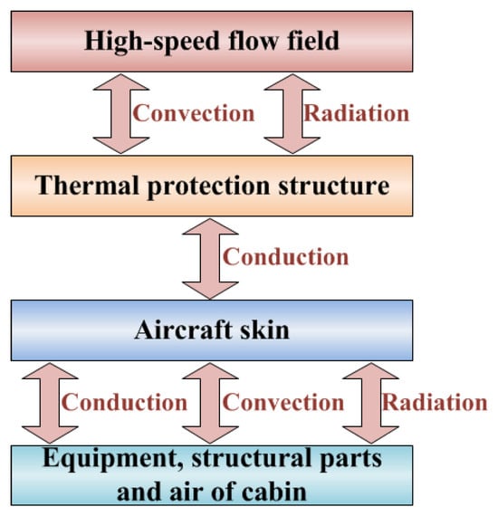
Figure 1. Physical processes involved in thermal analysis of high-speed vehicles.

Compared to the complex coupling mechanisms between the high-speed flow field and the TPS, as well as between the skin and internal thermal environment, the interaction between the TPS and the skin is relatively simple, based solely on heat conduction. Therefore, the contact surface between the TPS and the skin is selected as the coupled interaction interface. The high-speed flow field and the TPS are assigned to Partition 1, while the skin and internal thermal environment are assigned to Partition 2. Heat flux and temperature are chosen as the coupled interaction variables. Based on this, a thermal coupling analysis model for high-speed flight vehicles is established, as shown in Figure 2a.

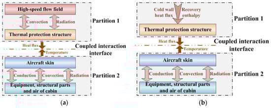
Figure 2. Thermal coupling modeling strategy for high-speed flight vehicles. (a) Thermal coupling analysis model; (b) Simplified thermal coupling analysis model.

In engineering practice, the calculation of high-speed aeroheating typically employs a decoupled computational strategy that proceeds from cold-wall heat flux to hot-wall heat flux. First, under the assumption of the wall temperature of 0 K, the cold-wall heat flux is computed using either engineering methods or numerical simulations [16]. Subsequently, during vehicle thermal analysis, this cold-wall heat flux is imported and converted into hot-wall heat flux (the actual aeroheating experienced by the vehicle) through correction formulas that account for real wall–temperature effects and wall–radiation heat transfer. This strategy decouples the complex aeroheating problem from the vehicle thermal analysis, allowing efficient and independent computation of core thermodynamic parameters in high-speed flow fields at relatively manageable computational cost. It avoids the substantial numerical burden and convergence difficulties associated with fully coupled thermal analyses while preserving computational accuracy. This approach ensures reliable and efficient transfer of aeroheating from high-speed flow field to the vehicle, providing an effective technical pathway for thermal analysis and thermal design of the vehicle that balances accuracy with feasibility.

This paper adopts the above strategy, and the aeroheating is simplified as boundary conditions that include cold-wall heat flux and recovery enthalpy. The simplified thermal coupling modeling strategy is shown in Figure 2b. The correction formula of cold-wall heat flux is shown in Equation (1), where the first term on the right side accounts for the real wall temperature effect, and the second term accounts for wall radiation heat transfer:

$$q_h(t)=q_c(t)(1-{\displaystyle \frac{T_w(t)+273.15}{T_h(t)+273.15}})-\epsilon \sigma {(T_w(t)+273.15)}^4$$

(1)

where q_h is hot-wall heat flux, [W/m²], which is the actual aeroheating experienced by the vehicle; q_c is cold-wall heat flux, [W/m²], which is the aeroheating under the assumption the wall temperature of 0 K; T_w is wall temperature, [°C]; T_h is recovery temperature derived from the recovery enthalpy, [°C]; t is time, [s]; ε is emissivity; σ is the Stefan–Boltzmann constant, 5.67 × 10⁻⁸ W/(m²·K⁴).

To ensure the prediction accuracy of the thermal response of high-speed vehicles, the implicit two-way coupling method is adopted. The thermal coupling analysis process is shown in Figure 3:

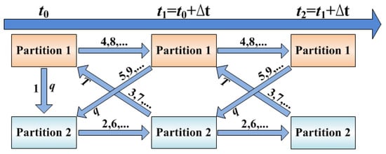
Figure 3. The two-way thermal coupling analysis process of high-speed flight vehicles (“…” denotes the third and subsequent iteration rounds).

• Based on the initial temperature field, perform the thermal analysis of Partition 1, and transfer the heat flux of the coupled interaction interface at time t0 from Partition 1 to Partition 2;
• Read the heat flux of the coupled interaction interface, perform the thermal analysis of Partition 2 from time t0 to (t0 + ∆t) to obtain the temperature distribution of the skin, equipment, structural components, and internal air domain at time t1;
• Transfer the temperature of the coupled interaction interface at time t1 from Partition 2 to Partition 1;
• Read the temperature of the coupled interaction interface, perform the thermal analysis of Partition 1 from time t0 to (t0 + ∆t) to obtain the hot-wall heat flux and temperature distribution of the TPS at time t1;
• Transfer the temperature of the coupled interaction interface at time t1 from Partition 1 to Partition 2;
• Repeat steps 2 to 5 until interaction variables satisfy the convergence criterion for iteration or reach the preset maximum number of iterations;
• Proceed to the next coupling time step until the preset end time is reached.

3. Mathematical Physics Model

The two-way thermal coupling analysis of high-speed vehicles involves transient conductive heat transfer within solid domains and between contacting solid domains, transient convective heat transfer between solid domains and internal air domains, transient radiative heat transfer between non-contacting solid domains, and the transfer and iteration of variables across partitions. To reduce model complexity, the following assumptions are made:

• Except for the TPS and printed circuit boards (PCB), the material of each component is uniformly distributed, isotropic, and the physical properties do not change with temperature.
• The electronic equipment cabin is an airtight compartment.
• The internal air is treated as an incompressible ideal gas, and the Boussinesq approximation is applied to account for buoyancy effects driven by temperature gradients. This simplification is based on the fact of an extremely low Mach number for internal natural convection (Ma < 0.3) and limited relative density change expected from the temperature rise (estimated < 10%). It is a common and effective approach for handling such natural convection problems in enclosed spaces. For extreme cases with very high temperature gradients within the cabin, the validity of this assumption would need re-evaluation, and a variable-density model should be employed for more precise analysis [17].
• The internal air does not participate in radiative heat transfer.
• All internal surfaces are assumed to be diffuse-gray. Although actual electronic component surfaces may exhibit non-gray or non-diffuse (specular) properties, employing representative average emissivity is a common engineering simplification in system-level thermal analysis.

3.1. Transient Conductive Heat Transfer Model

The transient conductive heat transfer within solid domains is modeled using Fourier’s law of heat conduction and the law of conservation of energy [18]:

$${\displaystyle \frac{{\rho }_s{c}_s}{{\kappa }_s}}{\displaystyle \frac{𝜕T_s}{𝜕t}}={\nabla }^2{T}_s+{\displaystyle \frac{{\theta }_s}{{\kappa }_s}}$$

(2)

where ρ is density, [kg/m³]; c is specific heat, [J/(kg·K)]; κ is thermal conductivity, [W/(m·K)]; T is temperature, [°C]; t is time, [s]; θ is volumetric power dissipation, [W/m³]; the subscript s represents solid domains.

The transient conductive heat transfer between contacting solid domains is described by the following:

$$\left\{\begin{array}{l}{q}_{s1-s2}=-{\kappa }_{s1}{A}_{s1-s2}{\left.{\displaystyle \frac{𝜕T_{s1}}{𝜕{\mathit{e}}_n}}\right|}_{\Gamma }={\kappa }_{s2}{A}_{s1-s2}{\left.{\displaystyle \frac{𝜕T_{s2}}{𝜕{\mathit{e}}_n}}\right|}_{\Gamma }\\ {\left.T_{s1}\right|}_{\Gamma }={\left.T_{s2}\right|}_{\Gamma }+r_{thCH}{A}_{s1-s2}\cdot (-{\kappa }_{s1}{\left.{\displaystyle \frac{𝜕T_{s1}}{𝜕{\mathit{e}}_{\mathrm{n}}}}\right|}_{\Gamma })\end{array}\right.$$

(3)

where q_s1-s2 is the conductive heat flux between contacting solid domains, [W/m²]; A_s1-s2 is the contact area between contacting solid domains, [m²]; r_thCH is the contact thermal resistance per unit area, [K/(W·m²)]; e_n is the normal direction to the interface; Γ is the contact interface; subscripts s1 and s2 represent the two solid domains that are in contact.

The contact surface between the solid domain and internal air domain is a boundary for convective and radiative heat transfer:

$$-{\kappa }_s{\left.{\displaystyle \frac{𝜕T_s}{𝜕{\mathit{e}}_n}}\right|}_{\Gamma }=h_{s-air}({\left.T_s\right|}_{\Gamma }-T_{air})+q_{rad-in,s}$$

(4)

where h_s-air is the convective heat transfer coefficient between the solid domain and internal air domain, [W/(m²·K)]; q_rad-in,s is the net absorbed radiative heat flux, [W/m²].

3.2. Natural Convective Heat Transfer Model in Confined Space

Natural convection is a fluid motion and heat transfer phenomenon driven by density differences induced by temperature gradients. An uneven temperature field leads to an uneven density field, which in turn generates the buoyancy force that drives natural convection. To simplify the solution of natural convective heat transfer, the Boussinesq approximation is introduced. This approximation considers density variation only in the buoyancy force term while treating density as constant in other terms, such as the continuity equation, the inertial and viscous terms in the momentum conservation equation, and the energy conservation equation [19]. Research indicates that under conditions where the fluid is incompressible and the temperature gradient is not significant, the Boussinesq approximation can accurately capture the effect of temperature variations on fluid motion while significantly reducing the complexity of natural convection problems. After introducing the Boussinesq approximation, the density of the internal air domain can be calculated by Equation (5), and the buoyancy force can be calculated by Equation (6):

$${\rho }_{air}={\rho }_{air-0}[1-{\beta }_{air}(T_{air}-T_{air-0})]$$

(5)

$$f_{buoyancy}=g{\beta }_{air}(T_{air}-T_{air-0})$$

(6)

where ρ_air-0 is reference density of air, [kg/m³]; β is thermal expansion coefficient, [K⁻¹]; T_air-0 is reference temperature of air, [°C]; f_buoyancy is buoyancy force, [N/kg]; g is gravitational acceleration, [m/s²]; the subscript air represents the air domain.

The solution of natural convective heat transfer in confined space involves the continuity equation, the momentum conservation equation, and the energy conservation equation [20]. The continuity equation describes mass transfer within the air domain:

$$\nabla \cdot {\mathit{U}}_{air}=0$$

(7)

where U is the velocity vector, [m/s].

The momentum conservation equation describes velocity transfer within the air domain:

$$\left\{\begin{array}{l}{\displaystyle \frac{𝜕u_{air}}{𝜕t}}+\nabla \cdot (u_{air}{\mathit{U}}_{air})=-{\displaystyle \frac{1}{{\rho }_{air}}}{\displaystyle \frac{𝜕{\mathrm{p}}_{air}}{𝜕x}}+{\displaystyle \frac{{\mu }_{air}}{{\rho }_{air}}}{\nabla }^2{u}_{air}+g_x{\beta }_{air}(T_{air}-T_{air-0})\\ {\displaystyle \frac{𝜕v_{air}}{𝜕t}}+\nabla \cdot (v_{air}{\mathit{U}}_{air})=-{\displaystyle \frac{1}{{\rho }_{air}}}{\displaystyle \frac{𝜕{\mathrm{p}}_{air}}{𝜕y}}+{\displaystyle \frac{{\mu }_{air}}{{\rho }_{air}}}{\nabla }^2{v}_{air}+g_y{\beta }_{air}(T_{air}-T_{air-0})\\ {\displaystyle \frac{𝜕w_{air}}{𝜕t}}+\nabla \cdot (w_{air}{\mathit{U}}_{air})=-{\displaystyle \frac{1}{{\rho }_{air}}}{\displaystyle \frac{𝜕{\mathrm{p}}_{air}}{𝜕z}}+{\displaystyle \frac{{\mu }_{air}}{{\rho }_{air}}}{\nabla }^2{w}_{air}+g_z{\beta }_{air}(T_{air}-T_{air-0})\end{array}\right.$$

(8)

where U is the velocity vector, u, v, w are components of U in x, y, z directions, [m/s]; p is the pressure, [Pa]; μ is the viscosity, [Pa·s]; g_x, g_y, g_z are components of the gravitational acceleration in x, y, z directions, [m/s²].

The energy conservation equation describes heat transfer within the air domain:

$${\rho }_{air}{c}_{air}({\displaystyle \frac{𝜕T_{air}}{𝜕t}}+{\mathit{U}}_{air}\cdot \nabla T_{air})={\kappa }_{air}{\nabla }^2{T}_{air}+{\theta }_{air}$$

(9)

where θ is viscous dissipation in fluid, [W/m³], representing the portion of mechanical energy converted into thermal energy due to viscous friction. In macroscopic scale flows, θ can be neglected; thus, θ_air = 0.

The interface between the internal air domain and the solid domains is a no-slip boundary:

$${\left.{\mathit{U}}_{air}\right|}_{\Gamma }=0$$

(10)

$${\left.T_{air}\right|}_{\Gamma }={\left.T_s\right|}_{\Gamma }$$

(11)

$$h_{s-air}({\left.T_{air}\right|}_{\Gamma }-\overline{T_{air}})=-{\kappa }_{air}{\left.{\displaystyle \frac{𝜕T_{air}}{𝜕{\mathit{e}}_n}}\right|}_{\Gamma }$$

(12)

3.3. Transient Radiative Heat Transfer Model in Confined Space

Radiative heat transfer refers to the process by which objects exchange heat through emission and absorption of electromagnetic waves. The amount of radiative heat transfer depends on factors such as temperature differences, surface emissivity, and the view factor between surfaces. The fundamental law governing the magnitude of radiative heat transfer is the Stefan–Boltzmann law. The actual radiative heat flux capability can be calculated based on corrections to the Stefan–Boltzmann law, as shown in Equation (13):

$$q_{rad}=\epsilon \sigma {(T+273.15)}^4$$

(13)

where q_rad is radiative heat flux, [W/m²]; ε is surface emissivity; T is temperature, [°C]; σ is Stefan–Boltzmann constant, 5.67 × 10⁸ W/(m²·K⁴).

For a closed space composed of n surfaces, the net absorbed radiative heat of surface k is the difference between the total absorbed radiative heat from other surfaces and the total emitted radiative heat to other surfaces, as shown in Equation (14):

$$Q_{rad-in,k}={\displaystyle \sum _{j=1}^{n-1}{A}_j{\epsilon }_j\sigma T_j^4{F}_{j,k}}-A_k{\epsilon }_k\sigma T_k^4$$

(14)

where Q_rad-in,k is the net absorbed radiative heat of surface k, [W]; A is area, [m²]; F_j,k is the view factor from surface j to surface k; the subscript k represents surface k; the subscript j represents surface j.

From the properties of the view factor,

$$A_k{F}_{k,j}=A_j{F}_{j,k}$$

(15)

where F_k,j is the view factor from surface k to surface j.

Substituting Equation (15) into Equation (14) yields the following:

$$q_{rad-in,k}={\displaystyle \sum _{j=1}^{n-1}{\epsilon }_j\sigma T_j^4{F}_{k,j}}-{\epsilon }_k\sigma T_k^4$$

(16)

Equation (16) shows that calculating the view factor is key to solving radiation heat transfer in a confined space. The Monte Carlo method can accommodate surface geometries of any shape, accurately handle complex occlusion relationships, and offer high computational stability with controllable error margins. Therefore, it is adopted in this study to calculate view factors between multiple surfaces inside the vehicle.

The Monte Carlo method is based on probability statistics and equates the radiative heat transfer process to random motion processes of photons, such as emission, projection, reflection, absorption, and scattering. By randomly sampling the microscopic behavior of photons and statistically processing the results, macroscopic radiative heat transfer characteristics can be obtained. This method was first applied to radiative heat transfer by Howell and Perlmutter [21]. Due to its advantages, such as a simple and clear physical model and flexible application, it has been widely adopted [22].

The basic steps for calculating the view factor from face i to face j using the Monte Carlo method are as follows [23,24]:

• Determine the geometric shape and position information of face i and face j.
• Set the total number of photons N_total emitted from face i, and initialize the counter N_i,j.
• Under consistent area-weighted probability conditions, randomly select a photon emission point P₁ on face i.
• Generate the emission direction d₁ based on Lambert’s cosine law.
• Emit a photon from P₁ along d₁. If it intersects with face j, increment the counter N_i,j by 1.
• After repeating steps 3 to 5 N_total times, the view factor F_i,j from face i to face j is calculated as F_i,j = N_i,j/N_total.

3.4. Variable Transfer Model at Coupling Interface

For the thermal coupling modeling strategy established in Section 2, the meshes of Partition 1 and Partition 2 typically have different topological structures and distribution densities, leading to non-corresponding grids at the coupling interface. This results in the challenge of accurate variable transfer between non-matching meshes, which is essentially an interpolation problem. For scalar-type variables, variables before and after interpolation should follow consistent spatial distribution rules; for vector-type variables, the variables before and after interpolation should also satisfy the flux conservation property. Therefore, this paper employs the radial basis function interpolation method for heat flux and the inverse distance weighting interpolation method for temperature.

3.4.1. Transfer Model for Heat Flux

Construct interpolation function f(x,y,z) with the following Equation:

$$\left\{\begin{array}{l}f(x,y,z)={\displaystyle \sum _{j=1}^m{\lambda }_j}\phi (‖\mathit{r}-{\mathit{r}}_j‖)\\ \phi (‖\mathit{r}-{\mathit{r}}_j‖)=\sqrt{{(x-x_j)}^2+{(y-y_j)}^2+{(z-z_j)}^2+{(1.25{\displaystyle \frac{D}{\sqrt{m}}})}^2}\end{array}\right.$$

(17)

where m is the number of nodes on the inner surface of the TPS; λ is weight coefficient matrix, λ = (λ₁, λ₂,…λ_m); φ(||r − r_j||) is basis function; r is direction vector; ||r − r_j|| is Euclidean distance from vector r to vector r_j, [m]; D is the diameter of node domain on the inner surface of the TPS, [m].

Substituting the heat flux q(x_i,y_i,z_i) of each node on the inner surface of the TPS into Equation (17) yields the linear equation system Equation (18). By solving Equation (18), the weight coefficient matrix λ is obtained. The heat flux q(X,Y,Z) of any node on the outer surface of the skin can be calculated using Equation (19):

$$q(x_i,y_i,z_i)={\displaystyle \sum _{j=1}^m{\lambda }_j\phi }(‖{\mathit{r}}_i-{\mathit{r}}_j‖)$$

(18)

$$\left\{\begin{array}{l}q(X,Y,Z)={\displaystyle \sum _{j=1}^m{\lambda }_j\phi }(‖\mathit{R}-{\mathit{r}}_j‖)\\ \phi (‖\mathit{R}-{\mathit{r}}_j‖)=\sqrt{{(X-x_i)}^2+{(Y-y_i)}^2+{(Z-z_i)}^2+{(1.25{\displaystyle \frac{D}{\sqrt{m}}})}^2}\end{array}\right.$$

(19)

where (x,y,z) is the coordinate of any node on the inner surface of TPS; (X,Y,Z) is the coordinate of any node on the inner surface of the skin.

3.4.2. Transfer Model for Temperature

Since the nodes on the outer surface of the skin are evenly distributed, a fixed number of nearest neighboring nodes is used for interpolation. Through debugging and cross-validation, it is found that selecting 30 nearest neighbors yields the optimal balance between accuracy and smoothness in the interpolation results. For any node (x,y,z) on the inner surface of the TPS, read the temperature of the 30 nearest neighboring nodes on the outer surface of the skin. Substituting them into Equation (20) yields the node temperature T(x,y,z):

$$\left\{\begin{array}{l}T(x,y,z)={\displaystyle \sum _{i=1}^{30}{w}_{i}T(X_i,Y_i,Z_i)}\\ w_i={\displaystyle \frac{{\sqrt{{(x-X_i)}^2+{(y-Y_i)}^2+{(z-Z_i)}^2}}^{-2}}{{\displaystyle \sum _{j=1}^{30}{\sqrt{{(x-X_j)}^2+{(y-Y_j)}^2+{(z-Z_i)}^2}}^{-2}}}}\end{array}\right.$$

(20)

where w is the weight coefficient.

3.5. Convergence Criterion for Thermal Coupling Iteration

$$\left\{\begin{array}{l}{\epsilon }_q={\displaystyle \frac{{\left({\displaystyle {\int }_{\Gamma }{\left(q_n^{m+1}-q_n^m\right)}^{2}d\Gamma }\right)}^{1/2}}{{\displaystyle {\int }_{\Gamma }{\left(q_n^m\right)}^{2}d\Gamma }}}\le 0.01\\ {\epsilon }_T={\displaystyle \frac{{\left({\displaystyle {\int }_{\Gamma }{\left(T_n^{m+1}-T_n^m\right)}^{2}d\Gamma }\right)}^{1/2}}{{\displaystyle {\int }_{\Gamma }{\left(T_n^m\right)}^{2}d\Gamma }}}\le 0.01\end{array}\right.$$

(21)

where ε_q is the iteration convergence criterion of heat flux; ε_T is the iteration convergence criterion of temperature; n is the time step for thermal coupling calculation; m is the sub-iteration count within the time step for thermal coupling calculation.

4. Thermal Coupling Analysis of the Electronic Equipment Cabin

4.1. Model

This section analyzes the heat flux transport characteristics and investigates the coupling mechanisms between internal and external thermal environments for the electronic equipment cabin shown in Figure 4, under long-duration and high-speed flight conditions. As shown in Figure 4a, the electronic equipment cabin has a length of 150 mm and a diameter of 300 mm, comprising components such as the TPS, the skin, stringers, the frame, the thermal battery module, the electronic module 1 (EM1), and the electronic module 2 (EM2). The TPS is made of phenolic resin-based ablative material with a thickness of 8 mm. The thermal battery is made of aluminum alloy and installed on a phenolic resin mounting plate. The quantity and layout of electronic components of both EM1 and EM2 are identical. However, electronic components of EM2 are tightly mounted against the module frame with a thermal conductive pad installed, enhancing heat transfer from electronic components to the frame, as shown in Figure 4b. The thermal property parameters of components of the electronic equipment cabin are detailed in Figure 5 and Table 1.

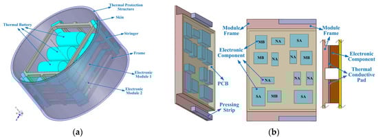
Figure 4. The electronic equipment cabin of a high-speed flight vehicle. (a) Structure composition of the electronic equipment cabin. (b) Structure composition of the electronic module.

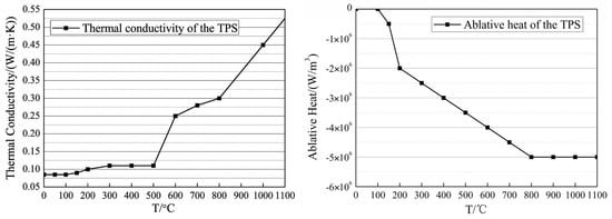
Figure 5. Thermal conductivity and ablative heat of the TPS.

Table 1. Thermal property parameters of the electronic equipment cabin.

Component	Density [kg/m3]	Specific Heat [J/(kg·K)]	Thermal Conductivity [W/(m·K)]	Emissivity	Power Dissipation [W]
TPS	980	1140	Figure 5	0.85	Figure 5
Skin	2800	904	142	0.20	-
Stringer	2800	921	121	0.20	-
Frame	2800	921	121	0.20	-
Thermal battery	2800	921	121	0.20
Mounting plate	1045	1500	0.2	0.85
Module frame	2800	921	121	0.20	-
Pressing strip	2800	921	121	0.20
PCB	2200	300	tangential: 32.5 normal: 0.8	0.85	-
SA 1	2800	1047	121	0.20	9.5
NA 1	4000	840	15	0.85	4.5
MB 1	900	800	10	0.85	6.4
Internal air domain	1.225	1006.4	0.0242	-	-

¹ The SA, NA, and MB are electronic components in EM1 and EM2.

The external thermal environment is shown in Figure 6, with a flight duration of about 1200 s, a peak cold-wall heat flux of about 500 kW/m², and a peak recovery enthalpy of about 2500 kJ/kg. The surface temperature of thermal batteries during the discharge process is shown in Figure 7, with a peak side-surface temperature of about 300 °C, and a peak terminal-surface temperature of about 240 °C. The initial temperature of the electronic equipment cabin is set to 60 °C.

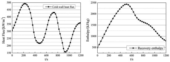
Figure 6. External thermal environment.

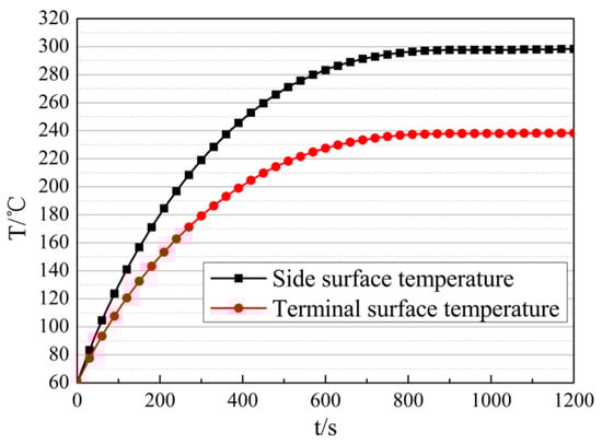
Figure 7. Surface temperature of the thermal battery during the discharge process.

4.2. Grid Independence Verification

The thermal coupling numerical calculation model is developed based on the commercial code Ansys Workbench, combined with user-defined programming. The model is discretized with a polyhedral mesh, as depicted in Figure 8. A grid independence study is carried out to balance computational cost and accuracy by determining the optimal number of grid cells. Three mesh schemes, summarized in Table 2, are evaluated by monitoring the temperature of device MB in EM1 and device NA in EM2. As shown in Figure 9, when the grid cell count exceeds 3,596,798, the temperature of MB and NA stabilizes with negligible fluctuations. Therefore, Meshing Scheme 2, shown in Table 2, is selected for all subsequent simulations.

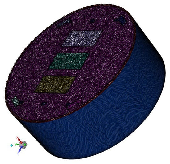
Figure 8. Schematic of mesh discretization.

Table 2. Meshing scheme.

Meshing Scheme	Minimum Size [mm]	Maximum Size [mm]	Grid Count
1	0.40	4.00	2,198,506
2	0.25	2.50	3,596,798
3	0.20	2.00	4,831,564

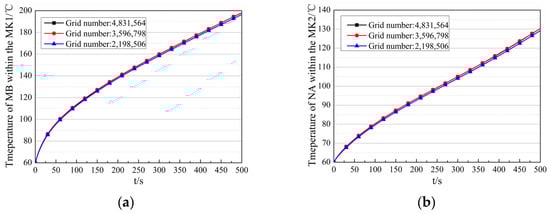
Figure 9. Grid independence verification. (a) Temperature of MB in the MK1 under different meshing schemes. (b) Temperature of NA in the MK2 under different meshing schemes.

4.3. Analysis of Heat Flux Transport Characteristics

At the end of the flight (t = 1200 s), the temperature distribution of the electronic equipment cabin is as shown in Figure 10. The temperature ranges from 195 °C to 466 °C, with the highest temperature observed in the TPS region, followed by the thermal battery and EM1 region. The temperature in the skin, frame, and EM2 region is relatively lower.

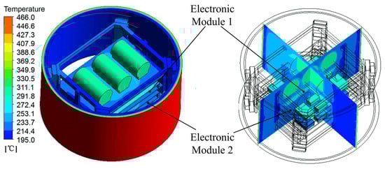
Figure 10. Temperature distribution of the electronic equipment cabin at the end of the flight.

The external surface temperature of the TPS and the maximum skin temperature during flight are shown in Figure 11a. The TPS temperature reaches a maximum of 911 °C, while the skin temperature peaks at 266 °C, below the maximum allowable temperature for aluminum alloy. The aeroheating and the aeroheating penetrated through the TPS are shown in Figure 11b. Both continue to increase during flight. The total aeroheating transferred into the electronic equipment cabin is 4465.07 kJ, with 398.03 kJ penetrating through the TPS. This indicates that the TPS blocked 91.09% of the aeroheating, demonstrating that the design of the 8 mm-thick phenolic resin-based ablative material TPS is effective.

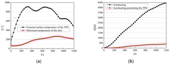
Figure 11. Thermal response characteristics of the TPS and the skin during flight. (a) External surface temperature of the TPS and maximum temperature of the skin. (b) Aeroheating and aeroheating penetrating the TPS.

The average temperature and enthalpy increment of structural components during flight are shown in Figure 12a,b. At the end of flight (t = 1200 s), the average skin temperature decreases to 207 °C, with an enthalpy increment of 160.54 kJ; the average temperature of stringers increases to 214 °C, with an enthalpy increment of 74.22 kJ; the average temperature of the frame increases to 214 °C, with an enthalpy increment of 94.4 kJ; and the average temperature of the air domain increases to 226 °C, with an enthalpy increment of 0.83 kJ.

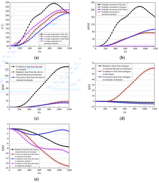
Figure 12. Thermal response characteristics of structural components during flight. (a) The average temperature of structural components and the air domain. (b) The enthalpy increment of structural components and the air domain. (c) The heat is transferred from the skin to the internal thermal environment. (d) The heat is transferred from the stringers to the internal thermal environment. (e) The heat is transferred from the frame to the internal thermal environment.

The heat transfer between structural components and the internal thermal environment is shown in Figure 12c–e. The total heat transferred from the skin to the internal thermal environment is 159.61 kJ, with 128.41 kJ transferred to stringers via conduction, accounting for 80.45%; 13.49 kJ transferred to the air domain via convection, accounting for 8.45%; and 17.71 kJ transferred to the internal thermal environment via radiation, accounting for 11.10%. The total heat transferred from stringers to the internal thermal environment is 54.17 kJ, with 60.84 kJ transferred to the frame via conduction, 4.62 kJ absorbed from the air domain via convection, and 2.05 kJ absorbed from the internal thermal environment via radiation. The total heat transferred from the internal thermal environment to the frame is 94.43 kJ, with 0.99 kJ absorbed from the EM1 via conduction, 9.97 kJ absorbed from the EM2 via conduction, 15.30 kJ absorbed from the air domain via convection, and 7.34 kJ absorbed from the internal thermal environment via radiation.

The heat flux transport within the electronic equipment cabin is summarized in Figure 13, and the analysis reveals the following:

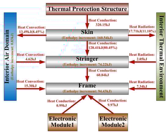
Figure 13. Schematic of heat flux transport within the electronic equipment cabin.

• The total aeroheating transferred into the internal thermal environment is 159.61 kJ, with conduction contributing 80.45%, convection contributing 8.45%, and radiation contributing 11.10%. This indicates that the aeroheating mainly affects the internal thermal environment through heat conduction.
• As the primary heat sink components, the frame and stringer experience a total enthalpy increase of 168.65 kJ. Of this, 128.41 kJ is absorbed from aeroheating via conduction, accounting for 76.14%; 10.96 kJ is absorbed from the electronic modules via conduction, accounting for 6.5%. Consequently, more than 76.14% of the heat sink capacity of stringers and the frame is consumed by aeroheating, which significantly impairs their ability to dissipate heat from electronic modules.
• The enthalpy increase in the air domain is only 0.83 kJ, indicating that the air domain has poor heat sink capacity and primarily acts as a heat transfer medium between components.

At the end of the flight (t = 1200 s), the temperature distribution of electronic modules is shown in Figure 14. The temperature of the EM1 ranges from 232 °C to 295 °C, while that of EM2 ranges from 224 °C to 234 °C. Compared to the EM1, the EM2 has a lower temperature rise and better temperature uniformity.

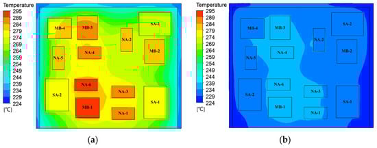
Figure 14. Temperature distribution of electronic modules. (a) Temperature distribution of the EM1. (b) Temperature distribution of the EM2.

The average temperature and enthalpy increment of components within the EM1 during the flight are presented in Figure 15a,b. At the end of the flight (t = 1200 s), the structural components (including module frame and pressing strips) reach an average temperature of 220 °C with an enthalpy increment of 48.57 kJ. In comparison, the PCB, MBs, SAs, and NAs exhibit higher average temperatures of 267 °C, 284 °C, 275 °C, and 286 °C, accompanied by enthalpy increments of 5.80 kJ, 3.70 kJ, 16.51 kJ, and 14.82 kJ, respectively. The resultant temperature differences between the structural components and MBs, SAs, and NAs are 65 °C, 55 °C, and 66 °C. This indicates that the thermal design of the EM1 fails to effectively utilize the heat sink capacity of the structural components.

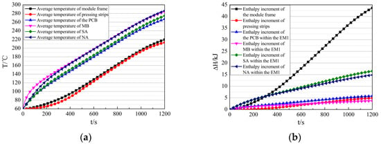
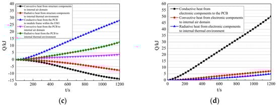
Figure 15. Thermal response characteristics of the EM1 during flight. (a) The average temperature of the components in the EM1. (b) The enthalpy increment of components in the EM1. (c) The heat transfer between structural components in the EM1 and the internal thermal environment. (d) The heat transfer between electronic components in the EM1 and the internal thermal environment.

The heat transfer between components within the EM1 and the internal thermal environment is shown in Figure 15c,d. The structural components absorb 13.80 kJ from the air domain via convection and 7.62 kJ from the internal thermal environment via radiation. The PCB within the EM1 transfers 28.11 kJ to structural components via conduction, transfers 3.68 kJ to the air domain via convection, and transfers 12.54 kJ to the internal thermal environment via radiation. The electronic components within the EM1 transfer 50.15 kJ to the PCB via conduction, transfer 7.14 kJ to the air domain via convection, and transfer 4.99 kJ to the internal thermal environment via radiation.

The heat flux transport within the EM1 is summarized in Figure 16, and the analysis reveals the following:

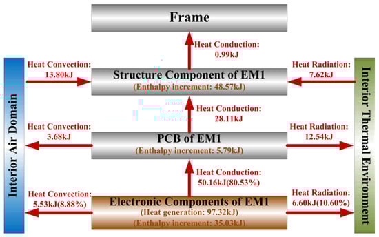
Figure 16. Schematic of heat flux transport within the EM1.

• The total heat generation in the EM1 is 97.32 kJ, with 0.99 kJ dissipated to the frame via conduction, accounting for 1.02%; with 6.94 kJ dissipated to the internal thermal environment via convection and radiation, accounting for 7.13%. This indicates that the thermal design of the electronic equipment cabin fails to effectively dissipate the heat generation within the EM1.
• The PCB absorbs 50.15 kJ from electronic components via conduction, with 5.79 kJ converted into its enthalpy increase, accounting for 11.55%. This suggests that the PCB possesses limited heat sink capacity.
• The total heat dissipated from electronic components within the EM1 is 62.28 kJ, of which 50.15 kJ (80.52%) is dissipated via conduction, 7.14 kJ (11.46%) is dissipated via convection, and 4.99 kJ (8.02%) is dissipated via radiation. This demonstrates that heat conduction serves as the primary and most effective dissipation mechanism for the electronic components. Therefore, the thermal management design of electronic modules should prioritize enhancing conductive heat transfer.

The average temperature and enthalpy increment of components within the EM2 during the flight are presented in Figure 17a,b. At the end of the flight (t = 1200 s), the structural components (including module frame and pressing strips) reach an average temperature of 228 °C with an enthalpy increment of 60.54 kJ. In comparison, the PCB, MBs, SAs, and NAs exhibit average temperatures of 233 °C, 236 °C, 235 °C, and 234 °C, accompanied by enthalpy increments of 4.82 kJ, 2.88 kJ, 13.19 kJ, and 11.51 kJ, respectively. The resultant temperature differences between the structural components and MBs, SAs, and NAs are 9 °C, 7 °C, and 6 °C. This indicates that the thermal design of the EM2 effectively utilizes the heat sink capacity of the structural components.

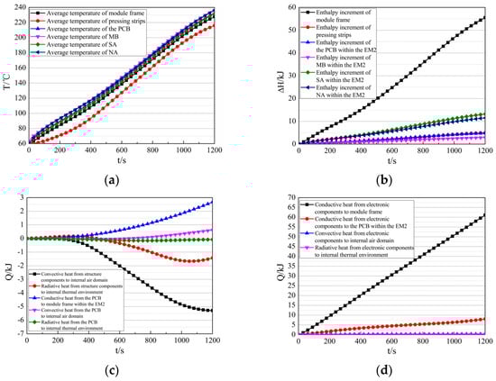
Figure 17. Thermal response characteristics of the EM2 during flight. (a) The average temperature of the components within the EM2. (b) The enthalpy increment of components within the EM2. (c) The heat transfer between structural components in the EM2 and the internal thermal environment. (d) The heat transfer between electronic components in the EM2 and the internal thermal environment.

The heat transfer between components within the EM2 and the internal thermal environment is shown in Figure 17c,d. The structural components absorb 5.29 kJ from the air domain via convection, and 1.43 kJ from the internal thermal environment via radiation. The PCB transfers 2.67 kJ to the module frame via conduction, transfers 0.62 kJ to the air domain via convection, and absorbs 0.08 kJ to the internal thermal environment via radiation. The electronic components within the EM2 transfer 61.12 kJ to the module frame via conduction, transfer 8.03 kJ to the PCB via conduction, transfer 0.32 kJ to the air domain via convection, and transfer 0.27 kJ to the internal thermal environment via radiation.

The heat flux transport within the EM2 is summarized in Figure 18, and the analysis reveals the following:

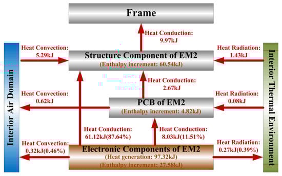
Figure 18. Schematic of heat flux transport within the EM2.

• The total heat generation in EM2 is 97.32 kJ, of which only 9.97 kJ (10.24%) is dissipated to the frame via conduction. This low proportion further confirms that the thermal design of the electronic equipment cabin fails to effectively dissipate the heat generation within electronic modules.
• Of the total 69.65 kJ dissipated from the electronic components within EM2, heat conduction serves as the dominant dissipation path: 61.12 kJ (87.75%) is dissipated to the module frame, while 8.03 kJ (11.54%) is dissipated to the PCB. In comparison, combined convection and radiation contribute only 0.59 kJ (0.71%).
• Compared with the EM1, the average temperature of the MBs, SAs, and NAs in the EM2 decreased significantly by 48 °C (16.9%), 40 °C (14.5%), and 52 °C (18.2%), respectively. These improvements confirm that mounting electronic components directly against the module frame with integrated thermal conductive pads can improve the utilization of the module’s heat sink capacity and substantially reduce the temperature rise in critical components.

4.4. Impact Analysis of Internal Power Dissipation

To analyze the impact of internal power dissipation, thermal coupling analysis was performed with the internal power dissipation increased to 2, 4, 6, and 8 times its original value. The results are compared in Figure 19. As illustrated in Figure 19a,b, both the aeroheating and the outer surface temperature of the TPS remain consistent across different internal power dissipation conditions. This suggests that these parameters are governed exclusively by the external aerodynamic thermal environment and the thermophysical properties of the TPS, independent of internal power dissipation.

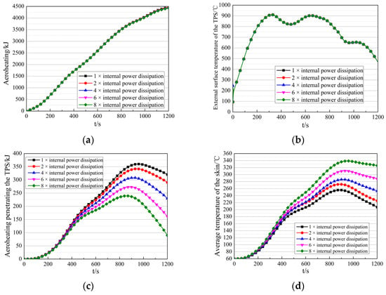
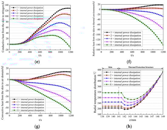
Figure 19. Results of thermal coupling analysis under different internal power dissipation conditions. (a) Comparison of the aeroheating. (b) Comparison of the outer surface temperature of the TPS. (c) Comparison of the aeroheating penetrating the TPS. (d) Comparison of the average skin temperature. (e) Comparison of the conductive heat transferred from the skin to the stringers. (f) Comparison of the radiative heat transferred from the skin to the internal thermal environment. (g) Comparison of the convective heat transferred from the skin to the air domain. (h) The radial temperature distribution across the TPS and the skin.

Figure 19c–g present comparisons of the aeroheating penetrating the TPS, the average skin temperature, and the heat transferred from the skin to the internal thermal environment. As internal power dissipation increases, several key trends are observed:

• The aeroheating penetrating the TPS decreases significantly, from 320.26 kJ to 290.50 kJ, 229.70 kJ, 161.78 kJ, and 89.66 kJ. This represents reductions of 9.3%, 28.3%, 49.5%, and 72.0%, respectively.
• The average skin temperature rises substantially, from 207 °C to 225 °C, 253 °C, 288 °C, and 326 °C. The corresponding increases are 18 °C, 46 °C, 81 °C, and 119 °C.
• The heat transfer from the skin to the internal environment is strongly suppressed and eventually reverses direction:

  ○

  Conductive heat to stringers drops from 128.41 kJ to 104.56 kJ, 62.22 kJ, 22.95 kJ, and −12.76 kJ.

  ○

  Radiative heat transfer drops from 17.71 kJ to 2.98 kJ, −28.01 kJ, −77.19 kJ, and −141.07 kJ.

  ○

  Convective heat to the air domain drops from 13.50 kJ to 6.00 kJ, −19.60 kJ, −40.11 kJ, and −57.62 kJ.

  ○

  The total heat transfer from the skin thus decreases from 159.62 kJ to 113.54 kJ, 14.61 kJ, −94.35 kJ, and −211.45 kJ (negative values indicate the skin absorbs heat from the internal environment).

Figure 19h shows the radial temperature distribution across the TPS and skin at the end of the flight (t = 1200 s). The temperature rise in the TPS region increases gradually along the radial direction, whereas the temperature increase in the skin region remains nearly uniform radially.

The analysis leads to the following conclusions:

• The aeroheating and the outer surface temperature of the TPS are governed exclusively by the external aerodynamic thermal environment and the thermophysical properties of the TPS, independent of internal power dissipation.
• Increasing internal power dissipation raises the internal temperature, thereby reducing the temperature gradient between the interior and exterior of the cabin. This suppresses both aeroheating penetration and heat transfer from the skin to the internal environment, indirectly elevating the temperature of the TPS and the skin.
• The temperature of the TPS and skin, the aeroheating penetrating the TPS, and the heat transfer from the skin to the internal environment all exhibit high sensitivity to increases in internal power dissipation, with relative changes exceeding the percentage increase in power dissipation itself.

4.5. Comparison of One-Way and Two-Way Thermal Coupling Analysis

The one-way thermal coupling model employs a sequential approach: it first analyzes the thermal response of the TPS and skin, assuming an adiabatic inner skin surface, then uses the penetrated aeroheating as the boundary condition to analyze the internal components. Taking the electronic equipment cabin shown in Figure 4 as the object, a comparison between the one-way and two-way thermal coupling analysis results is presented in Figure 20 and Table 3.

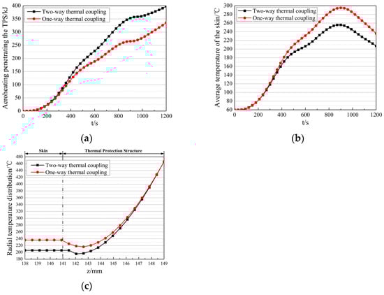
Figure 20. The comparison between the one-way and two-way thermal coupling analysis results. (a) Comparison of the aeroheating penetrating the TPS. (b) Comparison of the average skin temperature. (c) The radial temperature distribution across the TPS and the skin.

Table 3. Comparison of the temperature of electronic components.

Electronic Component	Two-Way Thermal Coupling	One-Way Thermal Coupling	Difference
MB 1 of EM1	285 °C	274 °C	11 °C
NA 1 of EM1	286 °C	275 °C	11 °C
SA 1 of EM1	275 °C	265 °C	10 °C
MB 1 of EM2	236 °C	220 °C	16 °C
NA 1 of EM2	236 °C	220 °C	16 °C
SA 1 of EM2	232 °C	216 °C	16 °C

¹ The SA, NA, and MB are electronic components in EM1 and EM2.

Significant deviations are observed between the one-way and two-way coupling results:

• For the aeroheating penetrating the TPS, the one-way model predicts 335.78 kJ, which is 62.23 kJ lower than the two-way model.
• For the maximum skin temperature, the one-way model predicts 295 °C, which is 39 °C higher than the two-way model.
• For the average temperature of electronic components in the EM1 (MBs, NAs, SAs), the one-way model predicts values lower than the two-way model by 11 °C, 11 °C, and 10 °C, respectively.
• For the average temperature of electronic components in the EM2 (MBs, NAs, SAs), the one-way model predicts values lower than the two-way model by 16 °C.
• In the TPS and skin region, temperatures from the one-way analysis are consistently higher than those from the two-way analysis, with the deviation increasing radially and stabilizing at 30 °C in the skin region.

The analysis leads to the following conclusions:

• The one-way thermal coupling analysis uses a serial iteration modeling strategy from external to internal, which fails to fully capture the interaction between inner and outer thermal environments. This leads to an overestimation of the temperature rise for the TPS and skin, and an underestimation for the electronic components. These predictive deviations accumulate with the duration of aeroheating and internal power dissipation.
• Overestimating the skin temperature leads to excessive design margin for the TPS, increasing vehicle weight and cost.
• Underestimating the temperature of electronic components leads to failure to identify overheating risks, reducing the reliability and safety of vehicle operation. Therefore, for long-duration and high-speed flight conditions, thermal analysis and design should be based on the two-way thermal coupling model.

4.6. Impact Analysis of Thermal Insulation Assembly Between the Skin and Stringers

From previous analyses, aeroheating entering the cabin consumes heat sink capacity, causing additional temperature rise in components and increasing thermal failure risk for sensitive devices. Since over 80% of aeroheating enters via conduction between the skin and stringers, reducing this heat flux is expected to preserve heat sink capacity. This section evaluates the benefit of installing thermal insulation pads between the skin and stringers.

Four types of thermal insulation pads, with materials of titanium alloy (TC4) and phenolic resin, and thicknesses of 2 mm and 4 mm, are analyzed. Their thermal properties are listed in Table 4.

Table 4. Thermal property parameters of thermal insulation pads.

Material	Density [kg/m3]	Specific Heat [J/(kg·K)]	Thermal Conductivity [W/(m·K)]
Titanium Alloy	4440	624	7.4
Phenolic Resin	1045	1500	0.2

The results of thermal coupling analysis for different thermal insulation pads are shown in Figure 21 and Table 5. All insulation pads reduce the aeroheating penetration and conductive heat transfer to the stringers, leading to lower electronic component temperatures. The phenolic resin pads, due to their lower thermal conductivity, perform significantly better than the titanium alloy pads:

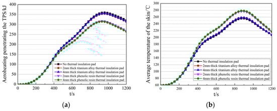
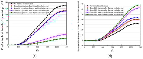
Figure 21. The results of thermal coupling analysis for different thermal insulation pads. (a) Comparison of the aeroheating penetrating the TPS. (b) Comparison of the skin temperature. (c) Comparison of the heat transferred from the skin to the stringers. (d) Comparison of heat transferred from the skin to the internal thermal environment via convection and radiation.

Table 5. Temperature of electronic components for different thermal insulation pads.

Electronic Component	No Thermal Insulation Pad	2 mm TC4	4 mm TC4	2 mm Resin	4 mm Resin
MB 1 of EM1	284 °C	281 °C	281 °C	270 °C	267 °C
NA 1 of EM1	286 °C	283 °C	283 °C	273 °C	271 °C
SA 1 of EM1	275 °C	271 °C	271 °C	259 °C	257 °C
MB 1 of EM2	236 °C	232 °C	232 °C	216 °C	214 °C
NA 1 of EM2	236 °C	232 °C	232 °C	216 °C	214 °C
SA 1 of EM2	232 °C	228 °C	227 °C	211 °C	209 °C

¹ The SA, NA, and MB are electronic components in EM1 and EM2.

• Compared to the non-insulated case, the aeroheating penetrating the TPS is reduced by 5.33 kJ (2 mm TC4), 7.14 kJ (4 mm TC4), 51.70 kJ (2 mm Resin), and 56.51 kJ (4 mm Resin).
• Conductive heat transfer from skin to stringers is reduced by 15.49 kJ (2 mm TC4), 16.85 kJ (4 mm TC4), 93.13 kJ (2 mm Resin), and 105.64 kJ (4 mm Resin).
• The average skin temperature increases slightly by 0.2 °C (2 mm TC4), 0.3 °C (4 mm TC4), 8 °C (2 mm Resin), and 10 °C (4 mm Resin), as less heat is dissipated.
• Temperature reductions for electronic components in the EM1 are 3 °C (2 mm TC4), 4 °C (4 mm TC4), 15 °C (2 mm Resin), and 17 °C (4 mm Resin).
• Temperature reductions for electronic components in the EM2 are 4 °C (2 mm TC4), 5 °C (4 mm TC4), 20 °C (2 mm Resin), and 23 °C (4 mm Resin).

The analysis leads to the following conclusions:

• Installing thermal insulation pads between the skin and stringers reduces both aeroheating penetration and conductive heat transfer from the skin to stringers. This decreases the consumption of heat sink capacity by aeroheating, lowers the temperature rise in electronic components, and improves their operational reliability.
• Both reducing the thermal conductivity and increasing the thickness of the thermal insulation pad enhance the suppression of aeroheating consumption. However, reducing thermal conductivity yields significantly greater benefits compared to increasing thickness.
• In the thermal design of high-speed vehicles, thermal insulation pads should be installed between the skin and stringers in cabins containing temperature-sensitive equipment to mitigate heat sink consumption by aeroheating. Pads with lower thermal conductivity should be prioritized, and their thickness should be appropriately increased.

5. Conclusions and Prospects

A two-way thermal coupling analysis model for high-speed vehicles under long-duration flight conditions is established using a partitioned modeling strategy. This study investigates the heat flux transport characteristics, the impact of internal power dissipation, the comparison between one-way and two-way thermal coupling analysis, and the benefits of thermal insulation between the skin and stringers. The results are intended to support accurate thermal response prediction and collaborative thermal design of high-speed vehicles. The main conclusions are as follows:

• The coupling effect of the external thermal environment on the internal thermal environment manifests as the consumption of internal heat sink capacity by aeroheating. This limits the component’s heat dissipation, causes additional temperature rise, and increases the risk of thermal failure. The coupling intensity increases with flight time and speed.
• The coupling effect of the internal thermal environment on the external thermal environment manifests as the suppression of aeroheating penetration, as well as heat transfer from the skin to the internal environment. The coupling strength is highly sensitive to increases in internal power dissipation.
• As more than 70% of heat transfer inside the electronic equipment cabin occurs via conduction, thermal design strategies should prioritize enhancing or inhibiting conductive heat transfer efficiency.
• For electronic modules, given the poor thermal capacity and conductivity of PCBs, measures such as mounting electronic components against the module structures with thermal conductive pads should be adopted to enhance heat dissipation, heat sink utilization, and module temperature uniformity.
• For cabins housing thermally sensitive equipment, thermal insulation pads should be installed between the skin and stringers to decrease the consumption of heat sink capacity by aeroheating. Pads with lower thermal conductivity should be prioritized, and their thickness should be appropriately increased.
• Thermal design based on one-way thermal coupling analysis, which fails to fully capture internal–external thermal interactions, leads to excessive margins in thermal protection design and inadequate internal thermal management design. Conversely, collaborative thermal design based on two-way coupling analysis is proven to achieve lighter weight, lower redundancy, higher reliability, and better safety. Therefore, for long-duration and high-speed flight conditions, thermal analysis and design of vehicles should be based on the two-way thermal coupling model.

The two-way thermal coupling model proposed in this paper provides an effective numerical approach for the thermal analysis of high-speed vehicle electronic equipment cabins. However, as a methodological investigation, the current work has not yet undergone direct experimental validation, which represents a notable limitation. In future research, we plan to construct a ground-based equivalent thermal test system using a quartz lamp array to simulate external aeroheating of typical-flight profiles. The temperature responses of key components, such as the skin and electronic modules, will be measured to validate and calibrate the thermal coupling model.

Several necessary simplifications are adopted in the modeling process, for instance, treating the internal air as an incompressible ideal gas and assuming all internal surfaces to be diffuse-gray. These simplifications help reveal the main physical mechanisms with acceptable computational complexity, though they may introduce some uncertainty into absolute temperature predictions. In subsequent work, we intend to develop a fully coupled CFD model and incorporate more precise surface radiation property data to support high-fidelity optimization design.

References

- Bertin, J.J.; Cummings, R.M. Fifty years of hypersonic: Where we’ve been, where we’re going. Prog. Aerosp. Sci. 2003, 39, 511–536. [Google Scholar] [CrossRef]
- Sziroczak, D.; Smith, H. A review of design issues specific to hypersonic flight vehicles. Prog. Aerosp. Sci. 2016, 84, 1–28. [Google Scholar] [CrossRef]
- Ding, Y.; Yue, X.; Chen, G.; Si, J. Review of control and guidance technology on hypersonic vehicle. Chin. J. Aeronaut. 2022, 35, 1–18. [Google Scholar] [CrossRef]
- Salas, M. A review of hypersonics aerothermodynamics and plasmadynamics activities within NASA’s fundamental aeronautics program. In Proceedings of the 39th AIAA Thermophysics Conference, Miami, FL, USA, 25 June 2007. [Google Scholar]
- Peng, Z.Y.; Shi, Y.L.; Gong, H.M.; Li, Z.H.; Luo, Y.C. Hypersonic aeroheating prediction technique and its trend of development. Acta Aeronaut. Et Astronaut. Sin. 2015, 36, 325–345. [Google Scholar]
- Jackson, T.A.; Eklund, D.R.; Fink, A.J. High speed propulsion: Performance advantage of advanced materials. J. Mater. Sci. 2004, 39, 5905–5913. [Google Scholar] [CrossRef]
- Song, K.D.; Choi, S.H.; Scotti, S.J. Transpiration cooling experiment for scramjet engine combustion chamber by high heat fluxes. J. Propul. Power 2006, 22, 96–102. [Google Scholar] [CrossRef]
- Marley, C.D. Thermal Management in a Scramjet Powered Hypersonic Cruise Vehicle. Ph.D. Dissertation, Aerospace Engineering. University Michigan, Ann Arbor, MI, USA, 2018. [Google Scholar]
- Uyanna, O.; Najafi, H. Thermal protection systems for space vehicles: A review on technology development, current challenges and future prospects. Acta Astronaut. 2020, 176, 341–356. [Google Scholar] [CrossRef]
- Yewei, G.U.I.; Lei, L.I.U.; Dong, W.E.I. Combined thermal phenomena issues of long endurance hypersonic vehicles. ACTA Aerodyn. Sin. 2020, 38, 641–650. [Google Scholar]
- Tabiei, A.; Sockalingam, S. Multiphysics coupled fluid/thermal/structural simulation for hypersonic reentry vehicles. J. Aerosp. Eng. 2012, 25, 273–281. [Google Scholar] [CrossRef]
- Jia, Z.X.; Wu, Z.G.; Wu, J.G.; Liu, Z.H.; Ren, F.; Hou, C.T. Study of two-way coupled fluid-structure-thermal analysis for hypersonic vehicles. Struct. Environ. Eng. 2019, 46, 17–23. [Google Scholar]
- Huang, J.; Yao, W.X.; Shan, X.Y. Integrated coupling analysis for hypersonic aerodynamic heating/structural temperature field. Mach. Des. Manuf. Eng. 2021, 50, 55–58. [Google Scholar]
- Wang, W.J.; Qian, W.; Bai, Y.G.; Wang, K.M. Numerical studies on the thermal-fluid-structure coupling analysis method of hypersonic flight vehicle. Therm. Sci. Eng. Prog. 2023, 40, 101792. [Google Scholar] [CrossRef]
- Chen, G.; Chen, W.D.; Ji, L.L.; Gao, T.S.; Lu, S.Z. Trajectory-based flow-thermal-structural coupling analysis for hypersonic vehicles. Phys. Fluids 2025, 37, 035192. [Google Scholar] [CrossRef]
- Hamilton, H.H.; Weilmuenster, K.J.; Dejarnette, F.R. Approximate method for computing convective heating on hypersonic vehicles using unstructured grids. J. Spacecr. Rocket. 2014, 51, 1288–1305. [Google Scholar] [CrossRef]
- Duan, C.A.; Bai, X.H.; Tang, Y.L.; Wang, Z.W.; Liu, C.L. Numerical study on the cooling characteristic of a novel laminated cooling configuration with chained beam turbulator in an afterburner heat shield. Int. Commun. Heat Mass Transf. 2025, 167, 109256. [Google Scholar] [CrossRef]
- Yang, S.M.; Tao, W.Q. Heat Transfer, 4th ed.; Higher Education Press: Beijing, China, 2006; pp. 115–123. [Google Scholar]
- Barletta, A. The Boussinesq approximation for buoyant flows. Mech. Res. Commun. 2022, 124, 103939. [Google Scholar] [CrossRef]
- Choi, S.K.; Kim, S.O. Turbulence modeling of natural convection in enclosures: A review. J. Mech. Sci. Technol. 2012, 26, 283–297. [Google Scholar] [CrossRef]
- Howell, J.R.; Perlmutter, M. Monte Carlo solution of thermal transfer though radiant media between gray walls. J. Heat Transf. 1964, 86, 547–560. [Google Scholar] [CrossRef]
- Fang, Q.Q.; Fang, W.; Yang, Z.L.; Yu, B.X.; Hu, H.B. A Monte Carlo method for calculating the angle factor of diffuse cavities. Metrologia 2012, 49, 572–576. [Google Scholar] [CrossRef]
- Liu, H.D.; Zhou, H.C.; Wang, D.D.; Han, Y.F. Performance comparison of two Monte Carlo ray-tracing methods for calculationg radiative heat transfer. J. Quant. Spectrosc. Radiat. Transf. 2020, 256, 107305. [Google Scholar] [CrossRef]
- Li, G.J.; Zhong, J.Q.; Wang, X.D. An improved Monte Carlo method for radiative heat transfer in participating media. J. Quant. Spectrosc. Radiat. Transf. 2020, 251, 107081. [Google Scholar] [CrossRef]
Disclaimer/Publisher’s Note: The statements, opinions and data contained in all publications are solely those of the individual author(s) and contributor(s) and not of MDPI and/or the editor(s). MDPI and/or the editor(s) disclaim responsibility for any injury to people or property resulting from any ideas, methods, instructions or products referred to in the content. |
© 2025 by the authors. Licensee MDPI, Basel, Switzerland. This article is an open access article distributed under the terms and conditions of the Creative Commons Attribution (CC BY) license.