Warping Deformation Prediction of Smart Skin Composite Airfoil Structure with Inverse Finite Element Approach

Abstract

The design of smart skin with lightweight requirements utilizes high-performance composite materials, resulting in thin structural characteristics. When subjected to complex aerodynamic loads, the smart skin structure experiences warping deformation, which significantly impacts both flight efficiency and structural integrity. However, this deformation behavior has been largely overlooked in current shape sensing methods embedded within the structural health monitoring (SHM) systems of smart skin, leading to insufficient monitoring capabilities. To address this issue, this paper proposes a novel shape sensing methodology for the real-time monitoring of warping deformation in smart skin. Initially, the structural displacement field of the smart skin and the warping function are mathematically defined, incorporating constitutive relations and considering the influence of material parameters on sectional strains. Subsequently, the inverse finite element method (iFEM) is employed to establish a shape sensing model. The interpolation function and the actual sectional strains, derived from discrete strain measurements, are calculated based on the current constitutive equations. Finally, to validate the accuracy of the proposed iFEM for monitoring warping deformation, numerical tests are conducted on curved skin structures. The results indicate that the proposed methodology enhances reconstruction capability, with a 10% improvement in accuracy compared to traditional iFEM methods. Consequently, the shape sensing algorithm can be seamlessly integrated into the SHM system of smart skin to ensure the predicted performance.

1. Introduction

Laminated composite (LC) smart skin, with numerous advantages such as light weight, high strength, and corrosion resistance, has found broad applications in various engineering fields, including aerospace [1], aircraft [2,3], navigation [4,5], and more. As a result, a significant number of researchers have been drawn to the development of laminated composite structures and the accurate prediction of their structural responses. This paper cites only a select few representative references, and for more comprehensive details, the reader is referred to [6]. The assessment of structural conditions is crucial in ensuring the safe operation of industrial equipment. Safety is particularly critical in aviation, where structural integrity is paramount, as a failure can often result in catastrophic consequences. For this reason, the structural health monitoring (SHM) technique is proposed for real-time assessment of structures. It utilizes real-time measurements, such as strain, acceleration, and temperature, from discrete sensors mounted on the structure to predict the health state of the structure [7,8]. This approach is effective in reducing operating costs and manpower, while improving overall structural safety [9]. Shape sensing technology is a critical component of SHM systems, providing robust technical support for the development of monitoring and control strategies for deformed structures. Structural shape sensing allows for real-time displacement reconstruction through discrete strain measurements, which highlights its nature as an inverse problem.

In recent years, various methods for anti-shape sensing problems have become a core research focus. This paper provides a brief overview and comparison of their main contributions. The structural kinematic variables, i.e., displacements and rotations, are predicted by integrating measured strains [10]. This methodology was originally proposed for plate elements and has been improved for beam and plate structures [11,12]. Additionally, the structural deformation field can also be regarded as a weighted superposition of basis functions [13]. However, this approach requires a priori interpolation basis functions or the vibrational mode shapes of the estimated structures [14], from which displacements can be determined by calculating the unknown weight coefficients from the discrete strain measurements [15]. In order to reduce the dependence of deformation monitoring on mathematical models and prior experience, an FBG-based approach, along with a data-driven and finite element model, has been proposed [16]. Among the various algorithms derived from existing literature, the inverse finite element method (iFEM) uses mathematical models to calculate structural displacement fields based on strain measurement results. Furthermore, this approach does not require any prior knowledge of material parameters or load conditions, but rather performs analysis based solely on strain measurement data. Moreover, it is convenient for the iFEM methodology to obtain strain measurements, where the strain sensors are typically bonded to the external surface of beam or plate structures [17]. Compared to the reconstruction methods mentioned above, the iFEM formulation has likely received the most widespread attention and recognition, as it is independent of interpolated shape functions or prior knowledge of the modal characteristics of structures and does not require an extensive model to produce reliable projections [18].

The iFEM approach was originally presented for shape sensing of plate and shell elements. As a result, many inverse-shell elements have been developed, including the three-node shell element (iMIN3) [19], four-node shell element (iQS4) [20], and the 8-node curved shell element [21]. These efforts have been further enhanced and applied to analyze composite structures, with engineering applications in wing-shaped geometries [22,23], stiffened panels [24,25], and marine structures [26,27]. Moreover, in order to avoid the non-invertibility of the reconstruction matrix, strain sensor placement optimization models have been established through a multi-objective particle swarm optimization algorithm [28,29]. Specifically, Ghasemzadeh et al. coupled iFEM with the genetic algorithm (GA) to reduce the number of sensors while maintaining displacement reconstruction accuracy [30]. Furthermore, the iFEM formulation has also been applied to detect damage in metallic and composite structures [31,32]. In addition, researchers such as Gherlone developed a theoretical method based on 1D iFEM to address the limitations of the 2D iFEM method in accurately reconstructing deformation in beams and frame structures [33]. Subsequently, this approach has been utilized to tackle cross-sectional complexities and composite structures [34]. The engineering performance of the 1D iFEM formulation has been demonstrated based on circular and airfoil beams [34], radio telescope reflectors [35], and subsea pipelines [36], among others.

In recent years, Zhao et al. coupled the iFEM with strain gradient theory to address geometrically nonlinear deformation problems of the Timoshenko beam, Euler-Bernoulli beam, and composite beam [37,38,39]. Li et al. developed an iterative linearization iFEM formulation based on the iQS4 unit, which predicts geometric nonlinear deformation by linearizing nonlinear responses [40]. To enhance the computational capability of nonlinear iFEM models, Wu et al. proposed an element-by-element iFEM approach constructed from the absolute nodal coordinate formulation (ANCF) [41].

Although previous shape sensing methods have been proven effective in many studies and supported by numerical calculations and experimental validations, their applicability to smart skin structures with warping deformations has not been thoroughly explored. This is particularly true for smart skin structures, especially in composite material structures, which exhibit different properties. Under loading, the anisotropic behavior of the materials leads to the simultaneous occurrence of bending, torsion, and warping. Due to the shear deformation of these multilayer materials, the cross-section undergoes warping, which significantly affects the overall deformation. However, traditional iFEM beam and shell models are typically based on classical beam theory (such as Euler–Bernoulli beam or Timoshenko beam theory), which assumes that the beam cross-section remains planar during deformation and does not account for warping deformations. In contrast, the method presented in this paper incorporates a more detailed geometric description and material response model, introducing a warping function that considers the effects of warping deformation on the cross-section.

To address this issue, a new iFEM method is proposed in this paper, specifically designed for modeling warping deformations in smart skin structures. This method effectively describes warping deformations in smart skins by defining a warping function and integrating it into the deformation theory of laminated smart skin structures. Validation results on a smart skin composite airfoil structure demonstrate that the proposed shape sensing model can accurately capture warping deformations, providing a new and more precise solution for shape sensing in smart skins.

The structure of the manuscript is delineated as follows: Section 2 reviews the displacement field theory, defines the warping function, and derives the constitutive equations. In Section 3, the shape sensing model is formulated based on the variational approach. Section 4 presents the determination of the reconstruction input, including the displacement interpolation functions and experimental section strain functions. Section 5 elaborates on the numerical calculations and experimental tests to validate the reconstruction accuracy of the proposed iFEM. The conclusions of this work, along with potential avenues for future investigation, are discussed in Section 6.

2. Basic Theory

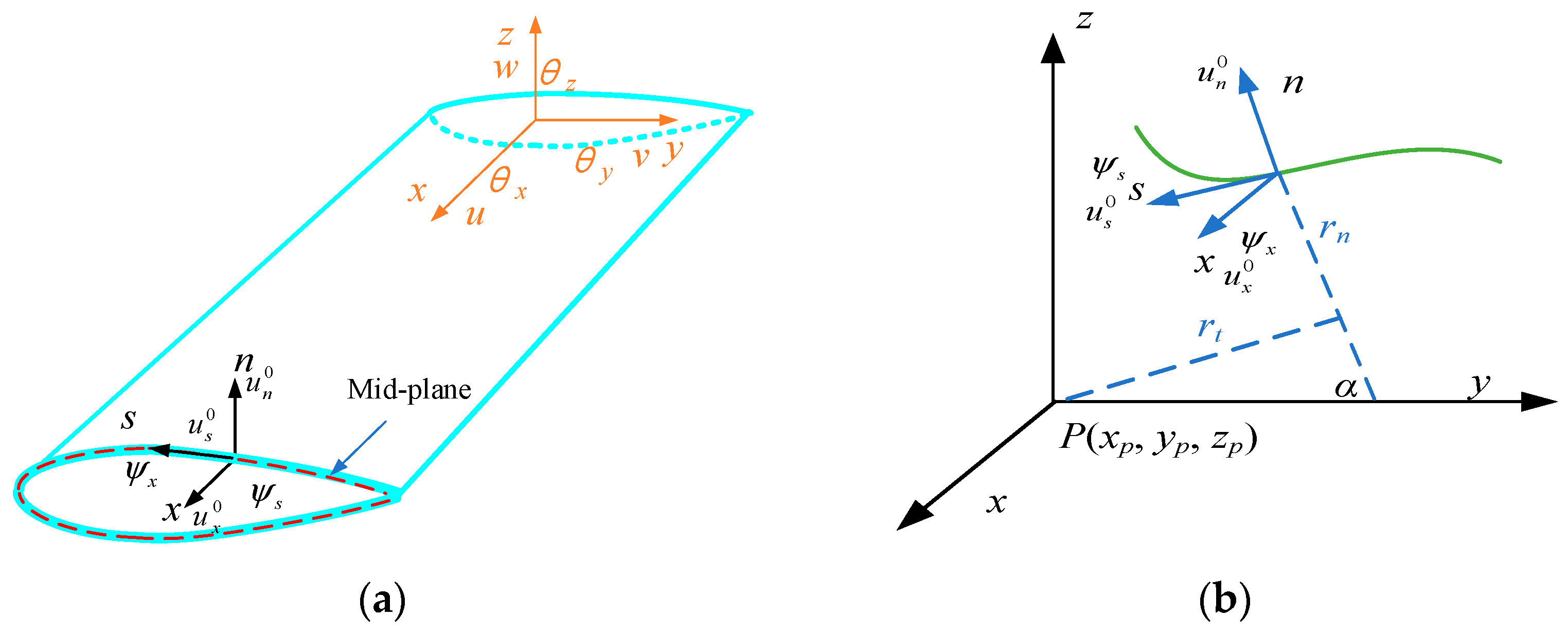
Consider a straight-line smart skin wing-shaped beam with a constant cross-sectional geometry. For the global structure, an orthogonal Cartesian coordinate system (x, y, z) is employed as the reference frame; for the local shell wall, a curvilinear coordinate system (x, s, n) is adopted, as presented in Figure 1. In each reference system, displacement and rotation are defined according to the forward direction of the coordinate axis. The pole P with coordinate (x_p, y_p, z_p) is the shear center of the airfoil cross-section (see Figure 1b). For the deformation description of the airfoil structure, the following assumptions are made:

Figure 1. Schematic of reference coordinate frames: (a) geometrical structure and kinematic variables; (b) local and global coordinate systems.

(i)

The cross-section contour of the airfoil structure is assumed to remain rigid within its own plane, with no consideration given to sectional distortion.

(ii)

After deformation, the normal on the undeformed median plane remains perpendicular to the deformed median plane.

(iii)

The warping function is defined with respect to point P or the central shear.

(iv)

The stress components σxx, σxs, and σxn, as well as the strains and curvature components εx, γxs, and γxn, are considered the most significant, and other components are assumed to be negligible.

According to small strain assumption theory, the mid-plane deformation of the shell wall can be expressed in terms of three Cartesian components of the displacement vector as follows:

$$\begin{array}{l}{u}_x^0(x,s,n)=u(x)+z(s)q_y(x)-y(s)q_z+{\varpi }_x(x,s,n)\\ u_s^0(x,s,n)=y_{,s}v(x)+z_{,s}w(x)+r_n(s){\theta }_x(x)\\ u_n^0(x,s,n)=z_{,s}v(x)-y_{,s}w(x)-r_t(s){\theta }_x(x)\\ {\psi }_x^0=-y_{,s}{\theta }_y-z_{,s}{\theta }_z+r_t{\theta }_{,x},{\psi }_s^0={\theta }_x\end{array}$$

(1)

where y_,s and z_,s are the trigonometric functions $-\mathit{sin}\alpha$ and $\mathit{cos}\alpha$, respectively. Angle α represents the orientation between n- and y-axes, as shown in Figure 1b. ($u_x^0$, $u_s^0$, $u_n^0$, ${\psi }_x^0$, ${\psi }_n^0$) are the kinematic variables of the shell mid-plane; (u, v, w, θ_x, θ_y, θ_z) are the global kinematic variables, which represent the displacements and rotations of the shell. The symbols r_n and r_t represent the normal and tangential coordinates of point P (x, y, z) on the shell mid-plane along n- and s-axes, respectively. By iterating through the local coordinates along the airfoil cross-section, the normal coordinate r_n and tangential coordinate r_t of any point can be calculated. ${\varpi }_x$ is an additional kinematic variable and is used to describe the warping deformation of the cross-section, which can be defined as follows:

$${\varpi }_x=-{\theta }_{x,x}\left({\displaystyle {\int }_0^s{r}_n(s)}\mathrm{ds}-{\mathrm{nr}}_t(s)\right)=-{\theta }_{x,x}p(s,n)$$

(2a)

where the functions r_n and r_t are expressed in the following form:

$$r_n(s)=Z(s){\displaystyle \frac{\mathit{dY}}{\mathit{ds}}}-Y(s){\displaystyle \frac{\mathit{dZ}}{\mathit{ds}}}; r_t(s)=Y(s){\displaystyle \frac{\mathit{dY}}{\mathit{ds}}}+Z(s){\displaystyle \frac{\mathit{dZ}}{\mathit{ds}}}$$

(2b)

with

$$y(s)=Y(s)-n{\displaystyle \frac{\mathit{dZ}}{\mathit{ds}}}; z(s)=Z(s)+n{\displaystyle \frac{\mathit{dY}}{\mathit{ds}}}$$

(2c)

The functions Z(s) and Y(s) are defined by the relationship between the arc length coordinate s and the global coordinates y and z, with the explicit form provided in the following sections. The coordinates y(s) and z(s) of a generic point in the cross-section are defined relative to the middle-line coordinates Y(s) and Z(s). Pursuant to the small-strain–displacement theory, the strain field is obtained

$$\begin{gathered} {\epsilon }_{\mathit{xx}}^0=u_{,x}+{z\theta }_{y,x}-{y\theta }_{z,x}+{\varpi }_{x,x}, {\gamma }_{\mathit{xs}}^0={\gamma }_{\mathit{xs}}^y+{\gamma }_{\mathit{xs}}^z+r_n{\theta }_{x,x}+{\varpi }_{x,s} \\ {\kappa }_{\mathit{xx}}={\psi }_{x,x}, {\kappa }_{\mathit{ss}}={\psi }_{s,s}, {\kappa }_{\mathit{xs}}={\psi }_{x,s}+{\psi }_{s,x}, \\ {\gamma }_{\mathit{xn}}=u_{n,x}^0+{\psi }_x, {\gamma }_{\mathit{xn}}=u_{n,s}^0+{\psi }_s \end{gathered}$$

(3a)

with

$${\gamma }_{\mathit{xs}}^y(x,s)=y_{,s}{v}_{,x}(x)-g_{,s}(s){\theta }_z(x)=G_0(s){\gamma }_{\mathit{xs},\mathit{max}}^y(x)$$

(3b)

$${\gamma }_{\mathit{xs}}^z(x,s)=z_{,s}{w}_{,x}(x)+f_{,s}(s){\theta }_y(x)=F_0(s){\gamma }_{\mathit{xs},\mathit{max}}^z(x)$$

(3c)

where transverse coordinates (y, z) can be expressed in terms of arc length coordinate s, such as z = f(s), y = g(s), which can be determined based on the cross-sectional shape of the specific airfoil structure. G₀ and F₀ are the distribution functions of the shear strains. Due to the two transverse shear loads, ${\gamma }_{\mathit{xs},\mathit{max}}^y$ and ${\gamma }_{\mathit{xs},\mathit{max}}^z$ refer to the maximal shear strains present at the contour coordinates of the cross-section, respectively. Furthermore, based on our previous research results [42], the strain terms ${\gamma }_{\mathit{xs},\mathit{max}}^y$ and ${\gamma }_{\mathit{xs},\mathit{max}}^z$ can be described by the section strains (e₄ and e₅) as follows:

$${\gamma }_{\mathit{xs},\mathit{max}}^y(x)={\displaystyle \frac{1}{k_{\epsilon y}}}{e}_5(x), {\gamma }_{\mathit{xs},\mathit{max}}^z(x)={\displaystyle \frac{1}{k_{\epsilon z}}}{e}_4(x).$$

(3d)

where $e_4(x)=w_{,x}(x)+{\theta }_z(x)$ and $e_5(x)=v_{,x}(x)-{\theta }_z(x)$. $k_{\epsilon y}$ and $k_{\epsilon z}$ are constant and are determined according to the presented calculation procedure in the literature [42]. Meanwhile, Equation (3a) can be expressed in another manner as follows:

$${\epsilon }_{\mathit{xx}}^0(x,s,n)=e_1(x)+z(s)e_2(x)-y(s)e_3(x)-p(s,n)e_{6,x}$$

(4a)

$${\gamma }_{\mathit{xs}}^0(x,s)={\displaystyle \frac{1}{k_{\epsilon y}}}{G}_0(s)e_5(x,s)+{\displaystyle \frac{1}{k_{\epsilon z}}}{F}_0(s)e_4(x,s)-{\mathit{nr}}_{t,s}(s)e_6(x)$$

(4b)

where e(u) = {e₁, e₂, e₃, e₄, e₅, e₆}^T are the theoretical section strains and are presented as

$$e_1(x)=u_{,x}(x), e_2(x)={\theta }_{y,x}(x), e_3(x)={\theta }_{z,x}(x), e_6(x)={\theta }_{x,x}(x),$$

(4c)

According to classical thin plate theory, the correlation between the resultant stress, stress coupling, and shell strain is given as follows [43]:

$$\left[\begin{array}{l}{N}_x\hfill \\ N_s\hfill \\ N_{\mathit{xs}}\hfill \\ M_x\hfill \\ M_s\hfill \\ M_{\mathit{xs}}\hfill \\ V_x\hfill \\ V_s\hfill \end{array}\right]=\left[\begin{array}{llllllll}{A}_{11}\hfill & A_{12}\hfill & A_{16}\hfill & B_{11}\hfill & B_{12}\hfill & B_{16}\hfill & 0\hfill & 0\hfill \\ A_{12}\hfill & A_{22}\hfill & 0\hfill & B_{12}\hfill & 0\hfill & 0\hfill & 0\hfill & 0\hfill \\ 0\hfill & 0\hfill & A_{66}\hfill & 0\hfill & 0\hfill & B_{66}\hfill & 0\hfill & 0\hfill \\ B_{11}\hfill & B_{42}\hfill & 0\hfill & D_{11}\hfill & D_{12}\hfill & 0\hfill & 0\hfill & 0\hfill \\ B_{42}\hfill & B_{11}\hfill & 0\hfill & D_{12}\hfill & D_{11}\hfill & 0\hfill & 0\hfill & 0\hfill \\ 0\hfill & 0\hfill & 0\hfill & 0\hfill & 0\hfill & D_{66}\hfill & 0\hfill & 0\hfill \\ 0\hfill & 0\hfill & 0\hfill & 0\hfill & 0\hfill & 0\hfill & {\mathit{kA}}_{44}\hfill & 0\hfill \\ 0\hfill & 0\hfill & 0\hfill & 0\hfill & 0\hfill & 0\hfill & 0\hfill & {\mathit{kA}}_{55}\hfill \end{array}\right]\left[\begin{array}{l}{\epsilon }_x\hfill \\ {\epsilon }_s\hfill \\ {\gamma }_{\mathit{xs}}\hfill \\ {\kappa }_x\hfill \\ {\kappa }_s\hfill \\ {\kappa }_{\mathit{xs}}\hfill \\ {\gamma }_{\mathrm{xn}}\hfill \\ {\gamma }_{\mathrm{sn}}\hfill \end{array}\right]$$

(5a)

$$N={[N_x,N_s,N_{\mathit{xs}}]}^T, M={[M_x,M_s,M_{\mathit{xs}}]}^T, V={[V_x,V_s]}^T$$

(5b)

$$\epsilon ={[{\epsilon }_x,{\epsilon }_s,{\gamma }_{\mathit{xs}}]}^T, \kappa ={[{\kappa }_x{,\kappa }_s,{\kappa }_{\mathit{xs}}]}^T, \gamma ={[{\gamma }_{\mathrm{xn}},{\gamma }_{\mathrm{sn}}]}^T$$

(5c)

where N, M, and V represent the resultant stress and couple of the laminated structure; ε contains the strains and shear strains in the x-s plane; κ represents the curvatures of the airfoil structure; γ is the shear strain in the x-n plane. The symbol k is the shear correction coefficient. A_ij, B_ij, and D_ij are the reduced stiffness components of materials referenced to the x-s-n coordinate system, which can be expanded in the following form:

$$\begin{array}{l}(A_{\mathit{ij}})={\displaystyle \sum _{r=1}^n{\tilde{Q}}_{\mathit{ij}}^{(r)}(h_r-h_{r-1})} \mathit{for} i,j=1,2,3\\ (D_{\mathit{ij}})={\displaystyle \frac{1}{3}}{\displaystyle \sum _{r=1}^n{\tilde{Q}}_{\mathit{ij}}^{\left(r\right)}(h_r^3-h_{r-1}^3)} \mathit{for} i,j=1,2,3\\ (B_{\mathit{ij}})={\displaystyle \frac{1}{2}}{\displaystyle \sum _{r=1}^n{\tilde{Q}}_{\mathit{ij}}^{(r)}(h_r^2-h_{r-1}^2)} \mathit{for} i,j=1,2,3\\ D_{44}={\displaystyle \frac{5}{4}}{\displaystyle {\int }_{h_{r-1}}^{h_r}{\tilde{Q}}_{44}^{(r)}\left[1-4{\left(\frac{z}{h}\right)}^2\right]}\mathit{dz},\\ D_{55}={\displaystyle \frac{5}{4}}{\displaystyle {\int }_{h_{r-1}}^{h_r}{\tilde{Q}}_{55}^{(r)}\left[1-4{\left(\frac{z}{h}\right)}^2\right]}\mathit{dz}\end{array}$$

(5d)

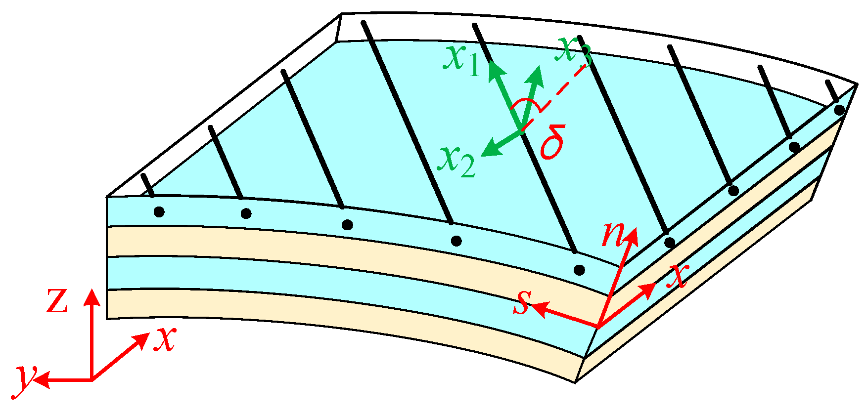
where n represents the overall number of layers in the wing structure; h_r and h_r−1 indicate the spacing from the shell reference surface to the outside and inside surfaces of the rth layer; $Q_{\mathit{ij}}^{(r)}$ is the transformed stiffness depending on the ply stiffness and fiber orientation δ, as shown in Figure 2, the specific matrix form can be found in [44]

Figure 2. Configuration of an n-layered airfoil beam.

These elastic material constants Q_ij are defined in the material coordinates (x₁, x₂, x₃) and are calculated based on the engineering constants, such as

$$Q_{11}={\displaystyle \frac{(1-{\mu }_{23}{\mu }_{32})}{\mathrm{\Pi }}}{E}_1, Q_{12}={\displaystyle \frac{({\mu }_{12}+{\mu }_{13}{\mu }_{32})}{\mathrm{\Pi }}}{E}_2, Q_{13}={\displaystyle \frac{({\mu }_{13}+{\mu }_{12}{\mu }_{23})}{\mathrm{\Pi }}}{E}_3$$

$$Q_{22}={\displaystyle \frac{(1-{\mu }_{13}{\mu }_{31})}{\mathrm{\Pi }}}{E}_2, Q_{23}={\displaystyle \frac{({\mu }_{23}+{\mu }_{21}{\mu }_{13})}{\mathrm{\Pi }}}{E}_3, Q_{33}={\displaystyle \frac{(1-{\mu }_{12}{\mu }_{21})}{\mathrm{\Pi }}}{E}_3$$

(5e)

$$Q_{44}=G_{13}, Q_{55}=G_{31}, Q_{66}=G_{12}$$

$$\mathrm{\Pi }={\displaystyle \frac{(1-{\mu }_{12}{\mu }_{21})}{\Pi }}{E}_3=1-{\mu }_{12}{\mu }_{21}-{\mu }_{23}{\mu }_{32}-{\mu }_{31}{\mu }_{13}-2{\mu }_{21}{\mu }_{32}{\mu }_{13}$$

where E is Yong’s modulus, G stands for the shear modulus, and μ stands for the Poisson ratio.

Furthermore, in the Cartesian coordinate system, the cross-section forces can be described in terms of the generalized beam strain and stiffness matrix (the derivative process can be found in reference [45]) as follows:

$$\mathbf{F}=\mathbf{Kq}$$

(6a)

in which

$$\mathbf{F}={\left[\begin{array}{lllllll}{F}_x\hfill & F_y\hfill & F_z\hfill & M_x\hfill & M_y\hfill & M_z\hfill & M_{\omega }\hfill \end{array}\right]}^T$$

(6b)

$$\mathbf{q}={\left[\begin{array}{lllllll}{u}_{,x}\hfill & {\gamma }_{\mathrm{xc},\mathit{max}}^y\hfill & {\gamma }_{\mathrm{xc},\mathit{max}}^z\hfill & {\theta }_{x,x}\hfill & {\theta }_{y,x}\hfill & {\theta }_{z,x}\hfill & {\theta }_{x,\mathrm{xx}}\hfill \end{array}\right]}^T$$

(6c)

Here, K is a (7 × 7) rearranged stiffness matrix, and non-zero elements can be defined as follows:

$$K_{11}=\left(A_{11}-{\displaystyle \frac{A_{12}^2}{A_{22}}}\right)b, K_{22}=kb{A}_{66}, K_{33}=kb{A}_{44}, K_{44}=4{\mathit{bD}}_{66}$$

(6d)

$$K_{55}=D_{11}-{\displaystyle \frac{D_{12}^2}{D_{22}}}, K_{66}={\displaystyle \frac{b^4}{12}}\left(A_{11}-{\displaystyle \frac{A_{12}^2}{A_{22}}}\right) K_{77}={\displaystyle \frac{b^3}{12}}\left(D_{11}-{\displaystyle \frac{D_{12}^2}{D_{22}}}\right)$$

(6e)

where b is the airfoil’s chord length. When the distributed loads q_x, q_y, and q_z are applied to the beam, the equilibrium equations are

$$F_{x,x}+q_x=0, F_{y,x}+q_y=0, F_{z,x}+q_z=0$$

$$M_{x,x}=0, M_{y,x}-F_z=0, M_{z,x}-F_y=0$$

(7a)

Combining Equations (6a) and (7a), the transformation relation can be obtained, as given by

$$e_5(x,s)={\displaystyle \frac{K_{55}}{K_{33}}}{e}_{2,x}=m_1{e}_{2,x}, e_4(x,s)={\displaystyle \frac{K_{66}}{K_{22}}}{e}_{3,x}=m_2{e}_{3,x}(x)$$

(7b)

3. iFEM Formulation for Airfoil Beams

In order to monitor the deformed shape of the airfoil beam structure, a least squares functional that matches the complete set of theoretical section strains, e(u), to the practical section strains, e^ε, is minimized with respect to the kinematic variables, u, which can be expressed as follows:

$$\mathbf{\Phi }={‖\mathbf{e}\left(\mathbf{u}\right)-{\mathbf{e}}^{\mathbf{\epsilon }}‖}^2$$

(8)

The airfoil beam can be discretized into elements. Thus, the element kinematic field in the pole-axes is calculated from an interpolation based on C⁰—continuous shape interpolation functions, i.e.,

$$\mathbf{u}(x)=\mathbf{N}(x){\mathbf{u}}^{\mathbf{e}}$$

(9)

where N(x) is the interpolation shape function, and u^e is the nodal degrees of freedom (DOF).

Then, plugging Equation (9) into Equation (4) yields the theoretical section strains in terms of DOF as

$$\mathbf{e}(x)=\mathbf{J}(x){\mathbf{u}}^e$$

(10)

where the matrix J includes the first derivatives of the shape function N(x). Equation (8) can be reformulated after the beam structure is discretized into n inverse-elements, as follows:

$${\mathrm{\Phi }}_k(x_i)={\displaystyle \frac{L}{n}}{\left[e_k(x_i)-e_k^{\epsilon i}\right]}^2(k=1–6)$$

(11)

where L stands for the length of the beam; x is the coordinate location for theoretical section calculation; the exponent εi represents the measured section strains, which are derived from the discrete surface strain measurements. Plugging Equation (10) into Equation (11) and then Equation (11) is able to be presented in quadratic form as follows:

$$\mathrm{\Phi }(x)={\displaystyle \frac{1}{2}}{({\mathbf{u}}^{\mathbf{e}})}^T{\mathbf{Ku}}^{\mathbf{e}}-{({\mathbf{u}}^{\mathbf{e}})}^T\mathbf{F}+{\mathbf{c}}^{\mathbf{e}}$$

(12)

where the parameter c^e is invariant. Meanwhile, matrices k^e and f^e are given by

$$\mathbf{K}={\displaystyle \sum _{k=1}^{1-6}{\mathbf{k}}_k^e} \mathbf{F}={\displaystyle \sum _{k=1}^{1-6}{\mathbf{f}}_k^e}$$

(13a)

and

$${\mathbf{k}}_k^e={\displaystyle \frac{L}{n}}{\displaystyle \sum _{i=1}^n\left({\mathbf{J}}_k^T{\mathbf{J}}_k\right)}, {\mathbf{f}}_k^e={\displaystyle \frac{L}{n}}{\displaystyle \sum _{i=1}^n\left(J_k^T{e}_k^{\epsilon i}\right)(k=1–6)}$$

(13b)

where matrices K and F are analogous stiffness matrix and load vectors, respectively. Matrix K is a function of section strain location x_i; the vector F is solely affected by the strain measurements. By minimizing function Φ and differentiating with respect to the nodal degrees of freedom u^e, a shape perception model can be obtained as follows:

$${\mathbf{Ku}}^{\mathbf{e}}=\mathbf{F}$$

(14)

The solution of the above equation for the unknown node DOF is efficient, which can be obtained based on the inverse operation of matrix K and the matrix–vector multiplication, u^e = K⁻¹F, where K⁻¹ remains unchanged for a set of determined strain sensor schemes.

4. Shape Functions and Experimental Section Strain Calculation

4.1. The NURBS Basis Functions

The non-uniform rational B-spline (NURBS) function is created by a linear combination of B-spline basis functions (R_i,p) and the corresponding control point (P_i). The basis functions are defined in a knot vector $\mathrm{\Xi }=[{\xi }_1,{\xi }_2,{\xi }_3,\dots {\xi }_i,\dots ,{\xi }_{n+p+1}]$, which is a set of non-decreasing numbers. Subscript n denotes the number of basis functions and control points, and p is the degree of the foundation functions. For an open knot vector, the knot is repeated p + l times at the first and last knots. The basis function can be defined recursively as follows:

$$R_{i,0}=\left\{\begin{array}{ll}1\hfill & {\xi }_i\le \xi \le {\xi }_{i+1}\hfill \\ 0\hfill & \mathit{otherwise}\hfill \end{array}\right.\mathrm{for} p=0$$

(15a)

and

$$R_{i,p}(\xi )={\displaystyle \frac{\xi -{\xi }_i}{{\xi }_{i+p}-{\xi }_i}}{R}_{i,p-1}(\xi )+{\displaystyle \frac{{\xi }_{i+p+1}-\xi }{{\xi }_{i+p+1}-{\xi }_{i+1}}}{R}_{i+1,p-1}(\xi ) \mathit{for} p\ge 1$$

(15b)

This paper employs the combination of basis functions and control points to describe the deformation fields, which are expressed as follows:

$$\mathbf{u}={\displaystyle \sum _{i=1}^n{R}_{i,p}{P}_i}=\mathbf{R}\mathbf{P}$$

(16)

where the order p of the basis function for the kinematic variables can be derived using the conclusion from Section 2. In Equation (6), when the section forces (F_x, F_y, F_z) and moments (M_x, M_y, M_z) are applied to the beam element, it can be concluded that e₁(i = 1, 6) are constants and e_i (i = 2, 3) follow a linear distribution by using Equations (6a) and (6b). Further, substituting the results into Equation (7b) shows that e_i (4, 5) are constants. It can be inferred that u and θ_x are linear functions, θ_y and θ_z are quadratic parabolic functions, and v and w are cubic polynomial functions. Among these, the longitudinal displacement function (y = z = 0) can be expressed as a basis function expansion:

$$\begin{array}{l}u={\displaystyle \sum _{i=1}^n{R}_{i,1}{u}_i}{\theta }_x={\displaystyle \sum _{i=1}^n{R}_{i,1}{\theta }_{\mathrm{xi}}}\\ {\theta }_y={\displaystyle \sum _{i=1}^n{R}_{i,2}{\theta }_{\mathit{yi}}}{\theta }_z={\displaystyle \sum _{i=1}^n{R}_{i,2}{\theta }_{\mathit{zi}}}\\ v={\displaystyle \sum _{i=1}^n{R}_{i,3}{v}_i}w={\displaystyle \sum _{i=1}^n{R}_{i,3}{w}_i}\end{array}$$

(17)

Furthermore, when the airfoil structure is subjected to uniformly distributed transverse loads (q_y, q_z), the section strains e_i (i = 2, 3) are parabolic, and e_i (i = 4, 5) are linear based on Equation (6) and Equation (7). Thus, v and w are quadratic, and θ_y and θ_z are cubic. Moreover, u and θ_x remain linear. Therefore, the displacement functions can be expressed as follows:

$$\begin{array}{l}{\theta }_y={\displaystyle \sum _{i=1}^n{R}_{i,3}{\theta }_{\mathit{yi}}}{\theta }_z={\displaystyle \sum _{i=1}^n{R}_{i,3}{\theta }_{\mathit{zi}}}\\ v={\displaystyle \sum _{i=1}^n{R}_{i,4}{v}_i}w={\displaystyle \sum _{i=1}^n{R}_{i,4}{w}_i}\end{array}$$

(18)

In order to ensure the expected C¹ continuity of twisting rotation (θ_x), as the strain vector (see Equation (4a)) comprises the second derivative of θ_x, this paper specifically uses a B-spline basis function of degree 3 to describe rotation distribution (refer to [46,47]):

$${\theta }_x={\displaystyle \sum _{i=1}^n{R}_{3,1}{\theta }_{\mathit{xi}}}$$

(19)

4.2. Section Strain Calculation

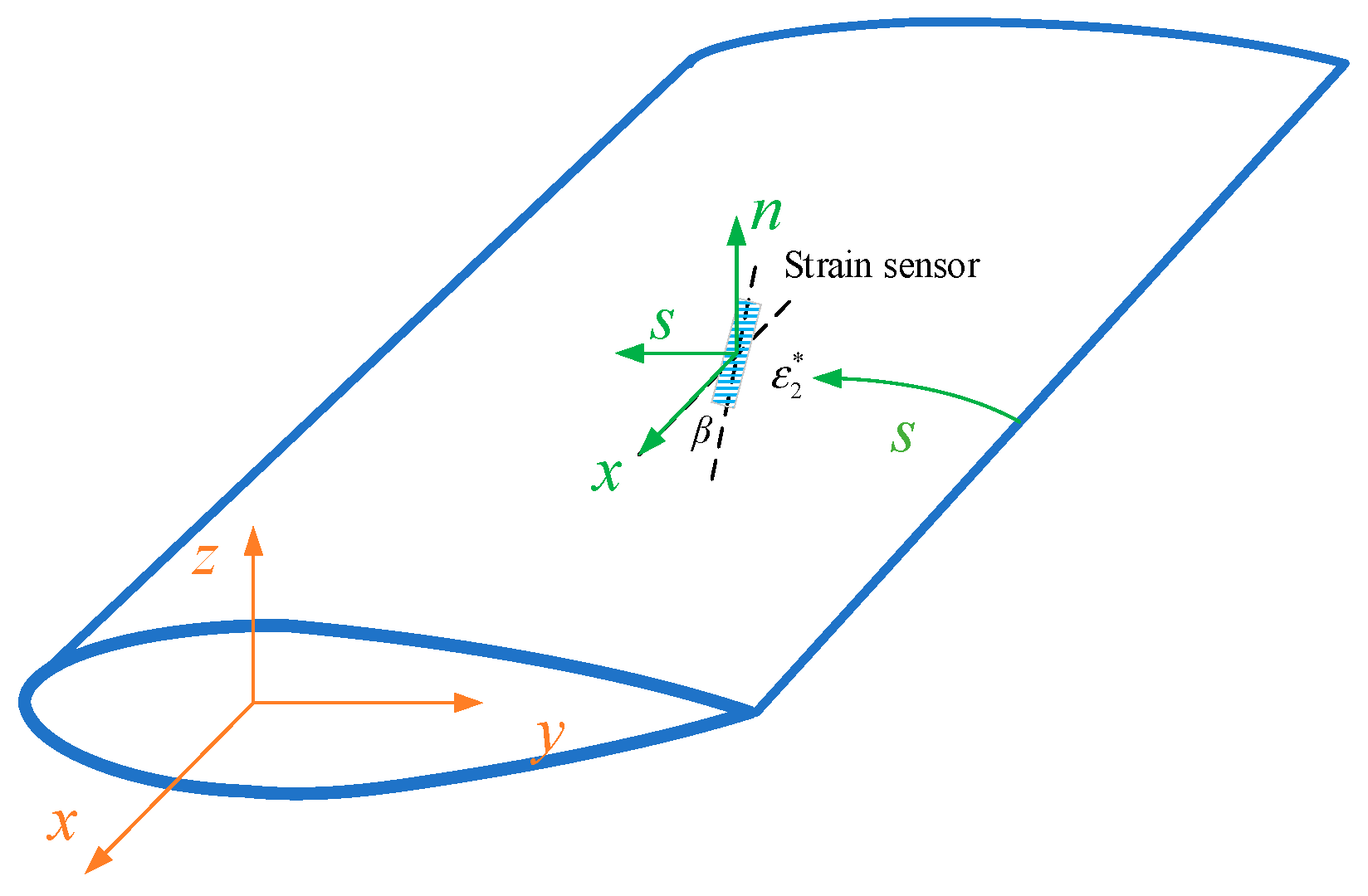
Calculating the experimental section strain e^ε from discrete surface strain measurements is a crucial step in the established iFEM formulations. In this section, the calculation process from the measured strain value to the four section strains is presented. To illustrate the procedure, the case study uses a thin airfoil structure. The Cartesian coordinate system (x, y, z) and curvilinear plane coordinate system (s, n) are shown in Figure 3.

Figure 3. Strain sensor location and its coordinate.

When a linear strain sensor is installed on the outer surface of the wing structure at position (x_i, y_i, z_i) or (x_i, s_i, n_i) and at an angle β to the wing axes, the relationship between the measured strain and the components of the plane strain tensor is given by the following formula:

$${\epsilon }_2^{*}={\epsilon }_x{\mathit{cos}}^2{\beta +\epsilon }_s{\mathit{sin}}^2{\beta +\gamma }_{\mathit{xs}}\mathit{cos}\beta \mathit{sin}\beta$$

(20a)

According to elastic deformation theory, Equation (20a) can be rewritten as

$${\epsilon }_2^{*}={\epsilon }_x\left({\mathit{cos}}^2\beta -{\mu \mathit{sin}}^2\beta \right)+{\gamma }_{\mathit{xs}}\mathit{cos}\beta \mathit{sin}\beta$$

(20b)

Then, substituting Equations (4a) and (4b) into Equation (20b) produces the relation between the measured strain and the four section strains is

$${\epsilon }_2^{*}(x_i,s_i,n_i,{\beta }_i)=\left(e_1+{\mathit{ze}}_2-{\mathit{ye}}_3-{\mathit{pe}}_{6,x}\right)\left(c^2\beta -{\mu s}^2\beta \right)+\left(G_0{m}_2{e}_{3,x}+F_0{m}_1{e}_{2,x}-{\mathit{nr}}_{t,s}{e}_6\right)c\beta s\beta$$

(20c)

where $c^2\beta ={\mathit{cos}}^2\beta$, $s^2\beta ={\mathit{sin}}^2\beta$, $c\beta =\mathit{cos}\beta$, and $s\beta =\mathit{sin}\beta$. When the strain sensors are positioned on the external surface and along the x-axis, where the angle β is 0, the relation can be simplified as follows:

$${\epsilon }_x^{*}(x_i,s_i,n_i)=e_1^{\epsilon }(x_i)+z(s_i)e_2^{\epsilon }(x_i)-y(s_i)e_3^{\epsilon }(x_i)-p(s_i,n_i)e_{6,x}^{\epsilon }(x_i)$$

(20d)

Meanwhile, according to the results deduced in Section 4.1, Equation (20) can be rewritten in terms of the matrix, such as

$${\epsilon }_{2i}^{*}(x_i,s_i,n_i)={\mathbf{POS}}_i(x_i,s_i,n_i)\cdot \mathbf{PAR}$$

(21a)

$$e^{\epsilon }(x_i)=\left[\begin{array}{l}{e}_1^{\epsilon }\hfill \\ e_2^{\epsilon }\hfill \\ e_3^{\epsilon }\hfill \\ e_{6,x}^{\epsilon }\hfill \end{array}\right]=\left[\begin{array}{lllllll}1\hfill & 0\hfill & 0\hfill & 0\hfill & 0\hfill & 0\hfill & 0\hfill \\ 0\hfill & x_i\hfill & 1\hfill & 0\hfill & 0\hfill & 0\hfill & 0\hfill \\ 0\hfill & 0\hfill & 0\hfill & x_i\hfill & 1\hfill & 0\hfill & 0\hfill \\ 0\hfill & 0\hfill & 0\hfill & 0\hfill & 0\hfill & x_i\hfill & 1\hfill \end{array}\right]\left[\begin{array}{l}{a}_1\hfill \\ a_2\hfill \\ a_3\hfill \\ a_4\hfill \\ a_5\hfill \\ a_6\hfill \\ a_7\hfill \end{array}\right]=C(x_i)\cdot \mathbf{PAR}$$

(21b)

with

$${\mathbf{POS}}_i=[1,x_i{z}_i,z_i,-x_i{y}_i,-y_i,-{\mathit{px}}_i,-p]\mathrm{and} e_6(x)={\displaystyle \frac{1}{2}}{a}_6{x}^2+a_{7}x+a_8$$

(21c)

where the subscript i denotes the ith strain sensor position. It can be seen from Equation (21b) that seven strain measurement values are needed to determine the unknown parameters a_i (i = 1–7), and the inverse solution is

$$\mathbf{PAR}={\mathbf{POS}}^{-1}{\epsilon }_2^{*}$$

(22)

where $\mathbf{POS}={[{\mathbf{POS}}_1,{\mathbf{POS}}_2,\dots ,{\mathbf{POS}}_6,{\mathbf{POS}}_7]}^T$, ${\epsilon }_2^{*}={\left[{\epsilon }_{21}^{*},{\epsilon }_{22}^{*},\dots ,{\epsilon }_{26}^{*},{\epsilon }_{27}^{*}\right]}^T$.

Therefore, substituting these parameters into Equation (21b) determines the section strains e_i (i = 1–3), and then substituting e₂ and e₃ into Equation (7b) presents e₄ and e₅ as follows:

$$e_5(x,s)=a_2{m}_1, e_4(x,s)=a_4{m}_2$$

(23)

where m_i (i = 1, 2) are known. Furthermore, when a linear strain sensor is placed at the airfoil surface with an angle β, the section strain e₆ can be determined by Equation (20c), i.e.,

$$e_6(x_i,s_i,n_i)=-\left({\displaystyle \frac{{\epsilon }_2^{*}-{\epsilon }_x^{*}}{\mathit{cos}\beta \mathit{sin}\beta }}-{\displaystyle \frac{1}{k_{\epsilon y}}}{G}_0{m}_2{a}_4-{\displaystyle \frac{1}{k_{\epsilon z}}}{F}_0{m}_1{a}_2\right)/{\mathrm{nr}}_{t,s}(s_i)$$

(24)

where ${\epsilon }_x^{*}(x_i,y_i,z_i)=\left(e_1(x_i)+z_i{e}_2(x_i)-y_i{e}_3(x_i)\right)\left({\mathit{cos}}^2\beta -{\mu \mathit{sin}}^2\beta \right)$. Then, combining the value $e_6(x_i,s_i,n_i)$ with Equation (21c) determines the unknown values a₈.

5. Applications

In this part, the finite element software is exploited to analyze the airfoil structure and thus verify the reconstruction accuracy of the proposed iFEM algorithm. The size of the airfoil is L = 2125 mm, width b = 200 mm, and height h = 25 mm. As presented in Figure 4, the airfoil structure is composed of a skeleton member and a skin, in which the composite stack is $[-{45}^{°} | {45}^{°} | 0^{°} | {45}^{°} | -{45}^{°} | -{45}^{°} | {90}^{°}]$_3s, and each layer is 0.3 mm thick. The mechanical property characteristics of the material are shown in Table 1, where E_i (i = x, y, z) is the elastic modulus, E_ij (i, j = x, y, z) is the shear modulus, and ${\mu }_{\mathit{ij}}\left(i,j=x,y,z\right)$ is Poisson’s ratio.

Figure 4. Composite material UAV wing structure: (a) finite element modeling and Cartesian coordinates; (b) finite element modeling and Cartesian coordinates.

Table 1. Performance parameters of composite wing skin materials.

Material Parameters	Ex (Gpa)	Ey	Ez	${\mathit{\mu }}_{\mathit{x}\mathit{y}}$	${\mathit{\mu }}_{\mathit{x}\mathit{z}}$	${\mathit{\mu }}_{\mathit{y}\mathit{z}}$	Gxy (Gpa)	Gxz	Gyz
Value	42.8	42.8	10.3	0.3	0.3	0.1	17.1	2.53	2.53

After modeling the composite airfoil in MSC Patran 2020 and establishing the 3D coordinate system (x, y, z) and local coordinate system (x, s, n) (shown in Figure 4a,b), shear and torsional loads are applied to the airfoil structure. The deformation field information can then be extracted from the analysis results.

5.1. Numerical Method for Calculating Coefficients and Variation Function

For a given airfoil structure, these variable functions {f₁, f₂, f₃} and parameters {k_εy, k_εz} can be further determined based on the results of the FE analysis, and their values are independent of the type and magnitude of external loads.

This section describes the specific solution steps: first, based on geometric principles, the transformation between the circumferential distance c of the airfoil and the coordinate y can be determined, as described by Equation (25).

$$\begin{array}{c}c\left(y\right)={\displaystyle \int \sqrt{1+{\left( d \prime \right)}^2}\mathit{dy}}\end{array}$$

(25)

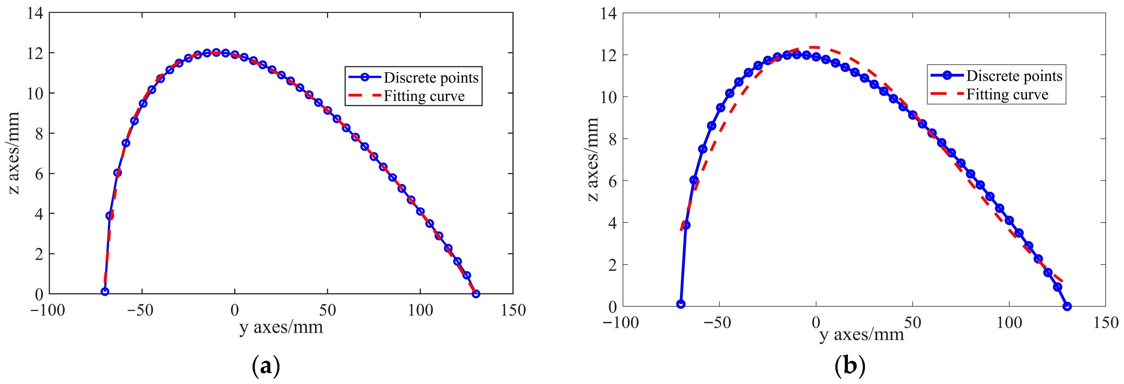
For the airfoil cross-sectional structure, the airfoil’s cross-sectional profile is represented by the function d(y), and the arc length c can be determined by the derivative of d(y). In this study, the coordinates of the nodes (x_i, y_i) on the section extracted from the finite element model are used to interpolate and fit d(y) using a 5/2 rational piecewise function. The geometric characteristics of the function d(y) and its mathematical expression are shown in Figure 5 and described by Equation (26) ($\begin{array}{c}y=\left(y-27.83\right)/60.88\end{array}$). Compared to traditional polynomial fitting methods, such as a third-order polynomial function, which exhibit significant errors in regions with large airfoil curvature, the 5/2 rational function provides a more accurate fit for complex airfoil geometries, particularly in regions with sharp bends and significant local geometric changes.

$$\begin{array}{c}d\left(y\right)=(-696y^5+645y^4-4750y^3-33090y^2+19903y+86350)/{(y}^2+4613y+8075)\end{array}$$

(26)

Figure 5. Fitted cross-section profile function image: (a) 5/2-times rational partition function; (b) third-degree polynomial function.

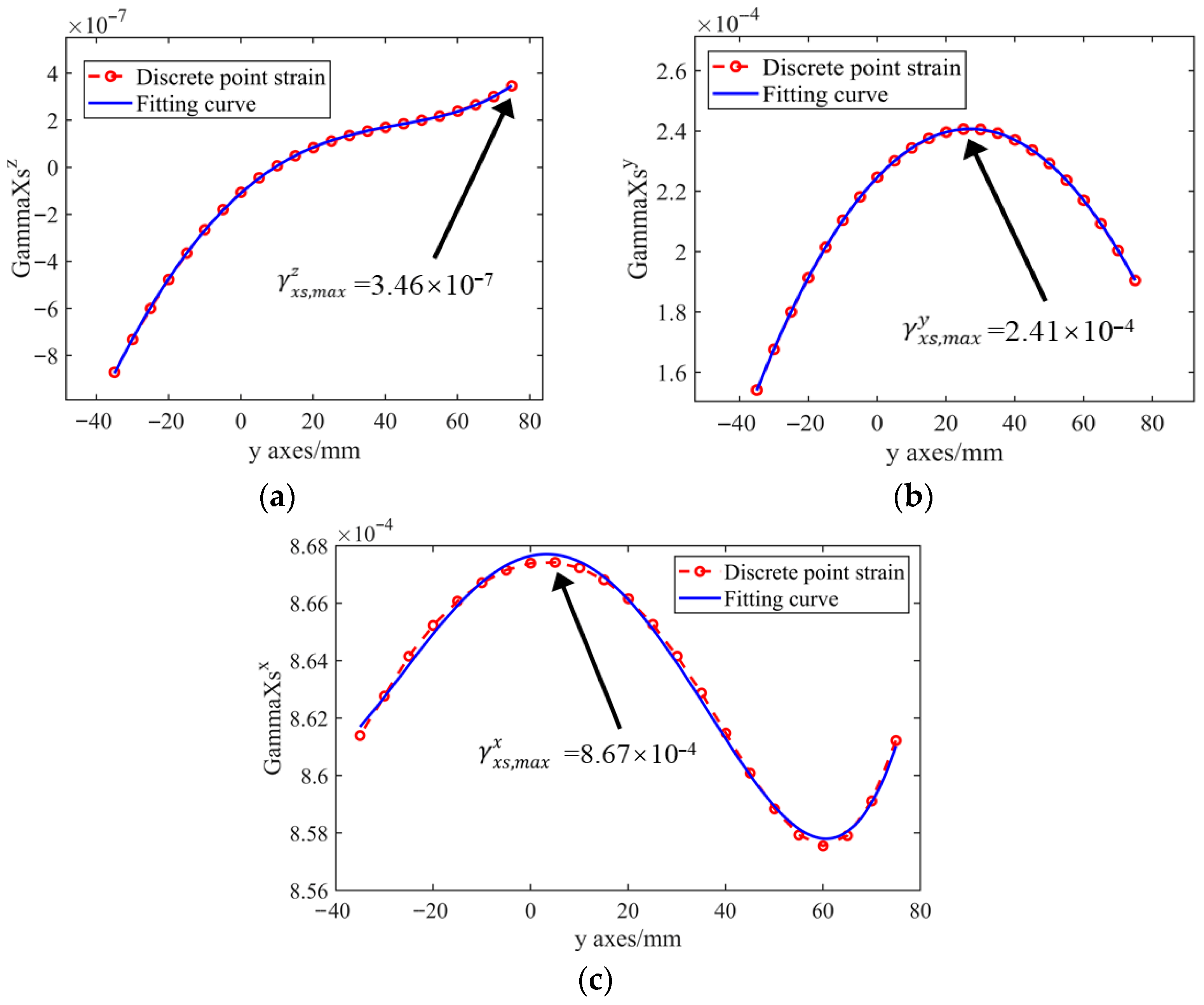
When shear loads and bending loads act separately on the wing structure, the shear strains ${\gamma }_{\mathit{xs}}^x$, ${\gamma }_{\mathit{xs}}^y$, and ${\gamma }_{\mathit{xs}}^z$ can be obtained at x_i = 1060 mm. By substituting the above shear strains and the cross-section angle function $\theta \left(k\right)=d_{,y}$ into Equation (27),

$$\begin{array}{c}{\gamma }_{\mathit{xs}}={\gamma }_{\mathrm{xy}}\left(c\right)\mathit{cos}\left(\theta \right)+{\gamma }_{\mathrm{xz}}\left(c\right)\mathit{sin}\left(\theta \right)\end{array}$$

(27)

Here, the shear strains ${\gamma }_{\mathit{xs}}^y\left(i\right)\left(i=1,2,\dots ,n\right)$ and ${\gamma }_{\mathit{xs}}^z\left(i\right)\left(i=1,2,\dots ,n\right)$ can be computed at all the nodes (see Figure 6 and Figure 7). For obtaining {f₁(c), f₂(c), f₃(c)} specifically, when load F_y or F_z is applied, the maximum value from the results of one iteration cycle is selected as ${\gamma }_{\mathit{xs},\mathit{max}}^y$ or ${\gamma }_{\mathit{xs},\mathit{max}}^z$. Combining this with Equation (28) allows f₂ and f₃ to be calculated; f₁ is obtained similarly.

$$\begin{array}{c}{f}_2\left(c\right)={\displaystyle \frac{{\gamma }_{xs}}{{\gamma }_{xs,max}^y}}\end{array}$$

(28)

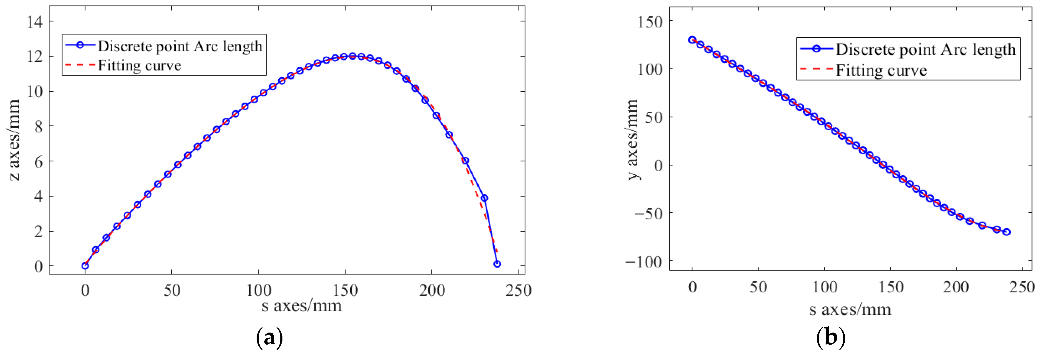
Figure 6. The relationship between arc length and cross-sectional coordinates: (a) Z(s); (b) Y(s).

Figure 7. Tangential shear strain distribution: (a) shear strain ${\gamma }_{\mathit{xs}}^z$; (b) shear strain ${\gamma }_{\mathit{xs}}^y$; (c) shear strain ${\gamma }_{\mathit{xs}}^x$.

Apply a unit torsional load M_x to the model and calculate f₁ using Equations (27) and (28).

Using the arc length formula, the arc length value corresponding to any point on the curve can be calculated. By associating this arc length value with the horizontal and vertical coordinates of the wing section, the functional relationships between arc length and the z-axis (Z(s)) and between arc length and the y-axis (Y(s)) are established and fitted with quartic polynomial curves, as shown in Equations (29) and (30). The fitting results are presented in Figure 6. Subsequently, substituting Equations (29) and (30) into Equation (2b), the r_n and r_t coordinates of any point P on the plane can be determined, thereby enabling the further derivation of the deformation function ${\varpi }_x$.

$$\begin{array}{c}Z\left(s\right)=-1.40\times {10}^{-8}{s}^4+3.02\times {10}^{-6}{s}^3-4.32\mathrm{e}\times {10}^{-4}{s}^2+0.123s+0.106\end{array}$$

(29)

$$\begin{array}{c}Y\left(s\right)=8.19\times {10}^{-8}{s}^4-2.87\times {10}^{-5}{s}^3+0.0025s^2-0.92s+130.9\end{array}$$

(30)

where s represents the arc length, while Z(s) and Y(s) represent the coordinate relationships of the cross-section along the z and y directions, respectively, as they vary with the arc length. The aforementioned polynomials are obtained through fitting and are used to describe the geometric distribution characteristics of the structure along the arc length direction.

$$\begin{array}{c}{f}_1^{\left(1\right)}\left(y\right)=4.53\times {10}^{-6}{y}^3-6.1\times {10}^{-4}{y}^2+0.037y-0.32\end{array}$$

(31)

$$\begin{array}{c}{f}_2^{\left(1\right)}\left(y\right)=3.15\times {10}^{-8}{y}^3-9.44\times {10}^{-5}{y}^2+0.05y+0.93\end{array}$$

(32)

$$\begin{array}{c}{f}_3^{\left(1\right)}\left(y\right)=1.13\times {10}^{-9}{y}^4-2.34\times {10}^{-8}{y}^3-6.55\times {10}^{-6}{y}^2+4.38\times {10}^{-5}y+1\end{array}$$

(33)

By substituting the variational functions $f_2^{(1)}$ = G₀ and $f_3^{(1)}$ = F₀, and the k_εy, k_εz obtained from [42] into Equation (24), the transformation relationship between the surface strain and the neutral axis strain can be established.

5.2. Verification of the iFEM Reconstruction Method

To validate the iFEM method, experimental studies were conducted on the airfoil structure under static loading conditions. Surface strain data were collected from the high-precision finite element model shown in Figure 4, with the extraction locations provided in Table 2. Using the deformation reconstruction model developed in this study, the wing displacement was reconstructed. To evaluate the load conditions that may be encountered in practical applications, two experimental setups involving shear and torsional loads were implemented to assess the reconstruction accuracy of the iFEM model under different loading conditions.

Table 2. Extracted surface strain point locations.

Strain Position Number	Strain Sensor Mounting Location
${\epsilon }_1$	$(1120\mathrm{mm},-30\mathrm{mm},12\mathrm{mm},0^{°})$
${\epsilon }_2$	$(1885\mathrm{mm},50\mathrm{mm},9\mathrm{mm},0^{°})$
${\epsilon }_3$	$(1090\mathrm{mm},-25\mathrm{mm},12\mathrm{mm},{45}^{°})$
${\epsilon }_4$	$(1530\mathrm{mm},20\mathrm{mm},11\mathrm{mm},0^{°})$
${\epsilon }_5$	$(1240\mathrm{mm},60\mathrm{mm},8\mathrm{mm},0^{°})$
${\epsilon }_6$	$(1685\mathrm{mm},40\mathrm{mm},10\mathrm{mm},0^{°})$
${\epsilon }_7$	$(385\mathrm{mm},45\mathrm{mm},10\mathrm{mm},{45}^{°})$

The sensor arrangement covers the entire span of the airfoil, including the leading edge, midsection, and trailing edge. This arrangement helps capture strain data at different locations on the airfoil, reflecting the varying load conditions experienced by the structure.

To comprehensively evaluate the reconstruction performance of the iFEM model proposed in this paper, this paper compares the Non-Warping-iFEM approach (based on classical beam theories such as Euler–Bernoulli and Timoshenko beams without considering warping deformation) with the Warping-iFEM approach (which accounts for warping deformation in this paper) under multiple loading conditions. The comparisons are conducted using displacement data extracted from Patran 2020 software. Additionally, this paper establishes evaluation criteria for reconstruction accuracy to quantify performance differences between the methods:

$$\begin{array}{c}\mathit{MER}=\mathit{Max}\left|{\mathit{disp}}^{\mathrm{reconstruction}}\left(x_i\right)-{\mathit{disp}}^{\mathit{PATRAN}}\left(x_i\right)\right|\end{array}$$

(34a)

$$\begin{array}{c}\mathit{RMS}=\sqrt{{\displaystyle \frac{1}{n}}{\displaystyle {\displaystyle \sum }_{i=1}^n}{\left({\mathit{disp}}^{\mathrm{reconstruction}}\left(x_i\right)-{\mathit{disp}}^{\mathit{PATRAN}}\left(x_i\right)\right)}^2}\end{array}$$

(34b)

$$\begin{array}{c}\mathit{RRMS}={\displaystyle \frac{\mathit{RMS}}{\mathit{Max}\left|{\mathit{disp}}^{\mathit{PATRAN}}\left(x_i\right)\right|}}\times \mathrm{100\%}\end{array}$$

(34c)

Here, the maximum absolute displacement error is denoted as MER, and disp(x) shows the displacement of each observation point along the longitudinal axes at the midpoint of the upper surface of the wing. The superscripts “reconstruction” and “PATRAN” refer to displacement data obtained using the deformation reconstruction method and Patran 2020 analysis, respectively. To further assess the accuracy of displacement estimation, the root mean square error (RMS) serves as an indicator; additionally, the relative root mean square error (RRMS) is introduced, defined as the proportion of the RMS value to the maximum displacement value in PATRAN analysis.

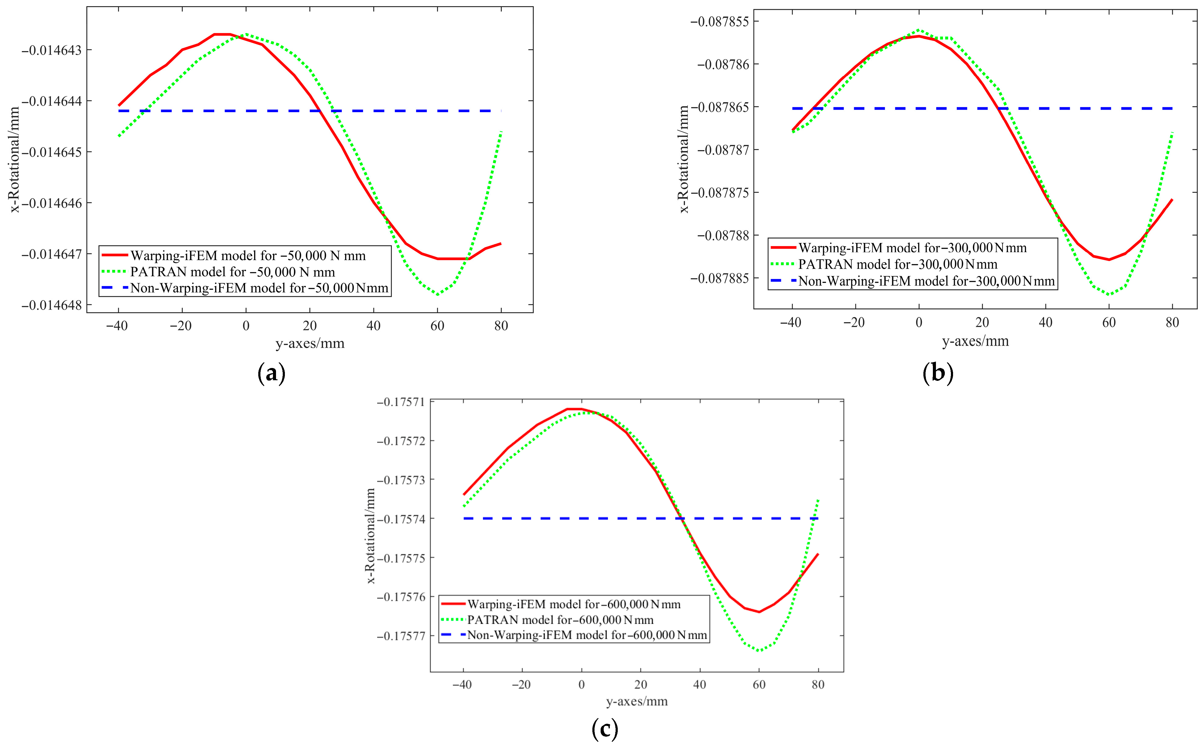
Under torsional loads, Figure 8a–c show significant warping deformation characteristics in the wing cross-section. According to the sectional twist angle results, the Warping-iFEM calculation exhibits a non-uniform distribution along the y-axis, which is highly consistent with the Patran 2020 results. In contrast, the Non-Warping-iFEM results approach a horizontal distribution, with significant deviations from the finite element solution, indicating that neglecting the warping effect underestimates the local torsional deformation. Furthermore, under different loading conditions (Mx = −50,000 N·mm, −300,000 N·mm, and −600,000 N·mm), the fluctuations in the twist angle caused by warping increase with increasing load, in accordance with the physical laws of structural twist deformation. Therefore, considering the warping effect is crucial for accurately predicting the torsional deformation of wing cross-sections.

Figure 8. Comparison of reconstructed rotation angle and theoretical rotation angle under torsional load: (a) Mx = −50,000 N·mm; (b) Mx = −300,000 N·mm; (c) Mx = −600,000 N·mm.

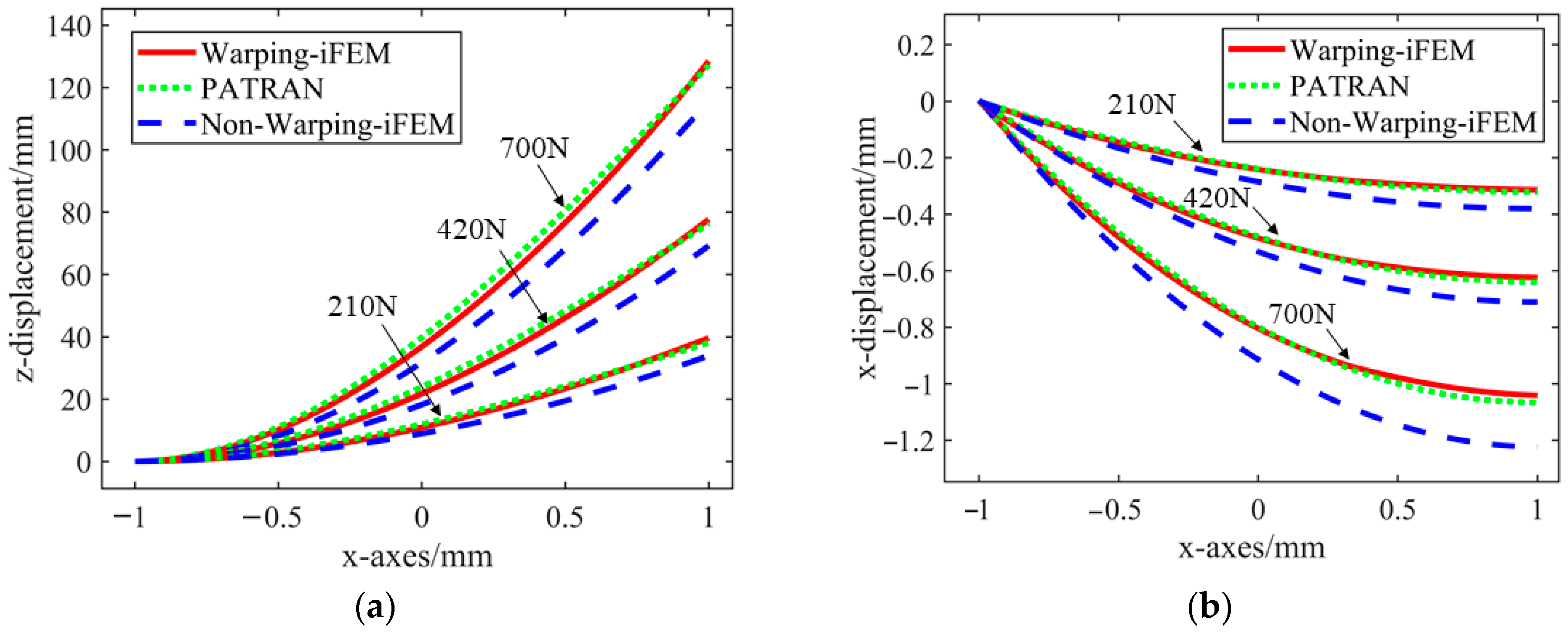
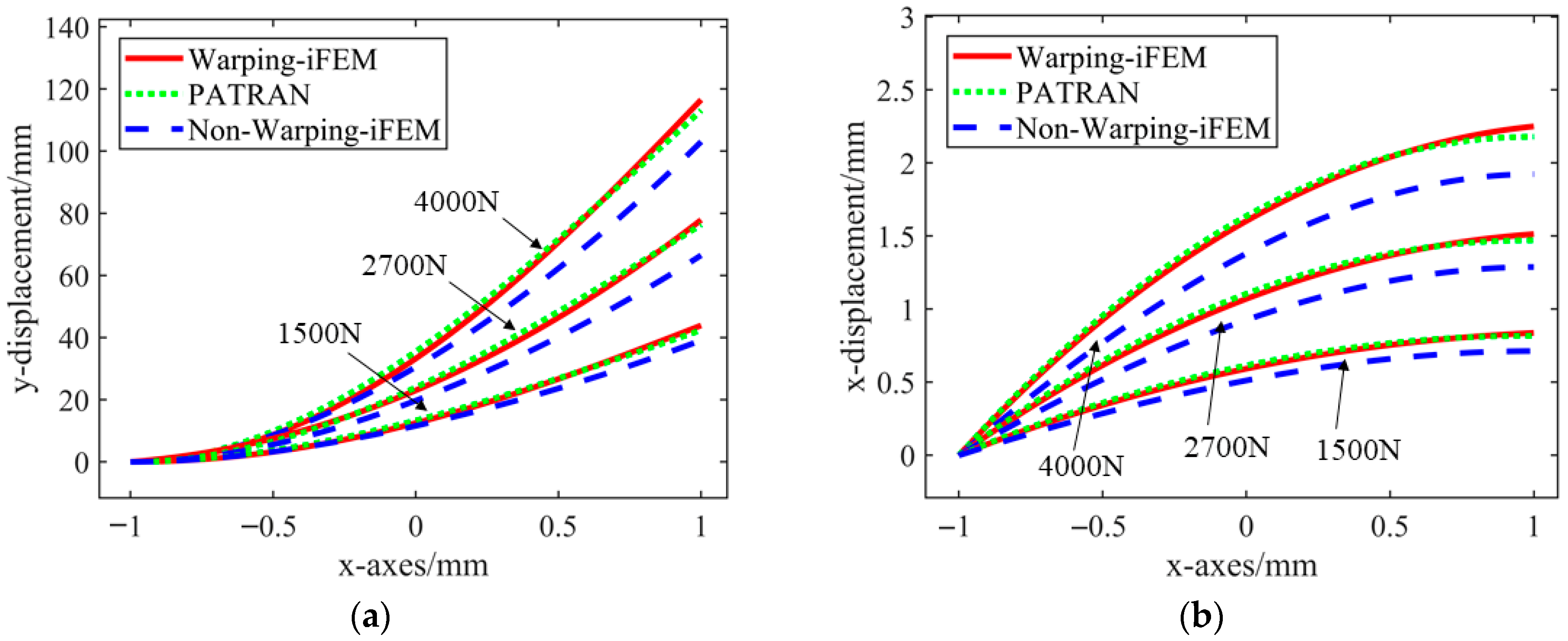
When applying concentrated loads, the Warping-iFEM method developed in this study and the conventional Non-Warping-iFEM method reconstruct displacement based on the obtained independent stress information (typically predicting times less than one second). Figure 9 and Figure 10 and Table A1, Table A2, Table A3, Table A4, Table A5 and Table A6 show the reconstruction accuracy analysis.

Figure 9. Comparison of reconstructed displacement and theoretical displacement under shear load in the Z direction: (a) z-axis displacement; (b) x-axis displacement.

Figure 10. Comparison of reconstructed displacement and theoretical displacement under shear load in the Y direction: (a) y-axis displacement; (b) x-axis displacement.

The figure shows a comparison of shear displacement in the Z direction. Figure 9a,b show that the reconstructed displacement is close to the theoretical displacement under the three applied loads.

Table A1, Table A2 and Table A3 show that the proposed Warping-iFEM method achieves significantly higher accuracy compared to the Non-Warping-iFEM strategy. Specifically, both MER and RRMS are significantly reduced. In the x-direction, MER decreased from approximately 0.16 mm to 0.013 mm, and RRMS decreased from nearly 12% to 1.78%; in the z-direction, MER decreased from approximately 12.63 mm to 3.85 mm, and RRMS decreased from 7.5% to 1.75%. Additionally, RRMS continued to decrease with increasing load, indicating that the influence of iFEM error weakens as deformation increases, with the error level ultimately converging to within 2%.

Figure 10 shows a comparison of shear displacement in the Y direction. Figure 10a,b show that the reconstructed displacement is close to the theoretical displacement under the three applied loads.

Similarly, as shown in Table A4, Table A5 and Table A6, the proposed Warping-iFEM significantly improves reconstruction accuracy. Specifically, both MER and RRMS are significantly reduced: in the x-direction, MER decreases from approximately 0.27 mm to 0.07 mm, and RRMS decreases from nearly 11% to 1.77%; in the y-direction, MER decreases from approximately 10.63 mm to 3.43 mm, and RRMS decreases from 7.58% to 1.77%. Additionally, as the load increases, RRMS continues to decrease, indicating that the iFEM error influence weakens as deformation increases, ultimately converging to within 2%.

In addition, Figure 9 and Figure 10 reveal that the Warping-iFEM method proposed in this paper more accurately matches the theoretical displacement curves in three directions (x, y, and z) compared to the conventional Non-Warping-iFEM strategy. In contrast, in the Non-Warping-iFEM method, the blue curve deviates significantly from the theoretical displacement. This is because the effects of distortion deformation on shear strain and wing beam section deformation have not been taken into account.

Due to unavoidable measurement errors caused by noise or the acquisition system in strain gauge measurements, to validate the reliability and robustness of the proposed Warping-iFEM method, measurement errors were simulated by introducing a randomly distributed normal noise signal into the extraction of surface strain information, as shown in Equation (33):

$${\epsilon }^{\mathrm{noisy}}={\epsilon }^{\mathrm{true}}\left(1+\mathrm{\Delta }r\right)$$

(35)

where ε^noisy and ε^ture represent strain data with and without noise influence, respectively; Δr denotes a Gaussian random number with mean 0 and standard deviation σ(Δr). Based on the method proposed in this paper, under the operating condition of F_z = 700 N, normally distributed noise signals with a mean of 0 and standard deviations of 1% and 2% of the strain were added. The reconstruction comparison results are shown in Table 3.

Table 3. Comparison of noise effects and actual results under F_z = 700 N. Unit: mm.

Method	PATRAN		Warping-iFEM-1%		Warping-iFEM-2%
Distance	x	z	x	z	x	z
85	−0.08	0.38	−0.0855	0.337	−0.0855	0.337
680	−0.57	17.51	−0.587	16.098	−0.587	16.029
850	−0.68	26.51	−0.693	24.364	−0.694	24.233
1020	−0.78	36.98	−0.784	34.047	−0.784	33.835
1360	−0.93	61.52	−0.921	57.351	−0.921	56.957
1700	−1.02	89.58	−0.996	85.705	−0.994	85.256
1955	−1.060	111.99	−1.029	110.423	−1.027	110.218
2040	−1.064	119.58	−1.035	119.377	−1.033	119.348
2125 (MD)	−1.066	127.24	−1.0388	128.710	−1.037	128.919
MER			0.031	4.167	0.033	4.561
RMS			0.0203	2.408	0.022	2.639
RRMS			1.90%	1.89%	2.02%	2.07%

The comparison results demonstrate that the Warping-iFEM method maintains high reconstruction accuracy even after introducing 1% and 2% noise. Although the MER and RMS in the x and z directions slightly increased with the elevated noise levels, the RRMS consistently remained between 1.90% and 2.07%. This demonstrates the method’s strong robustness to noise, enabling it to effectively handle measurement errors and validating its reliability and robustness for practical applications.

Based on all the analysis results presented above, it can be concluded that the Warping-iFEM model proposed in this paper demonstrates exceptional reconstruction capabilities, making it a reliable and precise tool for predicting the spatial state of UAV wing structures.

6. Conclusions

In response to the demand for accurate aircraft structural deformation sensing, this paper proposes an inverse finite element method (Warping-iFEM) for composite airfoils that explicitly accounts for cross-section warping, overcoming the limitations of traditional homogeneous or non-warping beam models. Based on theory for laminated composite beams, a cross-section strain–displacement relationship is constructed in which the shear strain distribution is described by the product of shear correction coefficients and variational functions. Subsequently, a dynamic conversion model was established between surface strain measurements and corrected cross-sectional strain, incorporating a warping function to capture warping deformation, thereby significantly enhancing reconstruction accuracy.

Experimental validation on a UAV wing beam under distributed loading shows that the proposed Warping-iFEM reduces transverse shear load reconstruction errors by more than 10% compared with conventional iFEM and achieves much better agreement with the theoretical displacement curves in all three directions (x, y, and z) than the Non-Warping-iFEM formulation. As evidenced by Table A4, Table A5 and Table A6, both MER and RRMS are markedly reduced. Moreover, when 1% and 2% normally distributed measurement noise are superimposed on the strain data, the reconstruction errors remain low, with RRMS consistently controlled at around 2% in the displacement components, demonstrating that the method maintains high accuracy and robustness under realistic measurement uncertainties. Overall, these results indicate that the Warping-iFEM model is a reliable and precise tool for predicting the spatial deformation state of UAV wing structures and offers a promising framework for real-time deformation feedback and structural health monitoring in aerospace, marine engineering, and civil structures under complex operating conditions.

References

1. Blala, H.; Lang, L.H.; Khan, S.; Li, L.; Sijia, S.; Guelailia, A.; Slimane, S.A.; Alexandrov, S. Forming challenges of small and complex fiber metal laminate parts in aerospace applications-a review. Int. J. Adv. Manuf. Technol. 2023, 126, 2509–2543. [Google Scholar] [CrossRef]
2. Mcgurk, M.; Stodieck, O.; Yuan, J. Probabilistic aeroelastic analysis of high-fidelity composite aircraft wing with manufacturing variability. Compos. Struct. 2024, 329, 117794. [Google Scholar] [CrossRef]
3. Ren, L.; Zhang, W.; Zhang, Y. Dynamic Snap-Through and nonlinear vibrations of bistable asymmetric Cross-Ply composite laminated cantilever shell under external excitation. Mech. Syst. Signal Process. 2023, 195, 110193. [Google Scholar] [CrossRef]
4. Pacheco-Blazquez, R.; Capua, D.D.; Garcia-Espinosa, J.; Casals, O.; Hakkarainen, T.; Tissari, A.; Korkealaakso, A. A new computational method for the assessment of the passive fire protection applied to a composite containership. Eng. Struct. 2023, 286, 116051. [Google Scholar] [CrossRef]
5. Jang, J.; Maydison, M.; Kim, Y. Effect of void content on the mechanical properties of GFRP for ship design. J. Mar. Sci. Eng. 2023, 11, 1251. [Google Scholar] [CrossRef]
6. Mittelstedt, C. Buckling and post-buckling of thin-walled composite laminated beams—A review of engineering analysis methods. Appl. Mech. Rev. 2020, 72, 020802. [Google Scholar] [CrossRef]
7. Simon, J.; Moll, J.; Krozer, V. Trend Decomposition for Temperature Compensation in a Radar-Based Structural Health Monitoring System of Wind Turbine Blades. Sensors 2024, 24, 800. [Google Scholar] [CrossRef] [PubMed]
8. Guo, Y.H.; Wang, K.; Leng, G.J.; Zhao, F.; Bao, H. Real-time temperature field reconstruction using a few measurement points and RPIM-AGQ6 interpolation. Measurement 2024, 225, 114041. [Google Scholar] [CrossRef]
9. Sofla, A.Y.N.; Meguid, S.A.; Tan, K.T.; Yeo, W.K. Shape morphing of aircraft wing: Status and challenges. Mater. Des. 2010, 31, 1284–1292. [Google Scholar] [CrossRef]
10. Ko, W.L.; Richards, W.L.; Tran, V. Displacement Theories for In-Flight Deformed Shape Predictions of Aerospace Structures; NASA/TP-2007-214612; NASA: Washington, DC, USA, 2007.
11. Smoker, J.; Baz, A. Monitoring the bending and twist of morphing structures. Sens. Smart Struct. Technol. Civ. Mech. Aerosp. Syst. 2008, 6932, 69321X. [Google Scholar]
12. Heaney, P.S.; Ivanco, T.G.; Bilgen, O. Distributed sensing of a cantilever beam and plate using a fiber optic sensing system. In Proceedings of the 2018 Applied Aerodynamics Conference, Atlanta, GA, USA, 25–29 June 2018; pp. 1–28. [Google Scholar]
13. Kim, N.S.; Cho, N.S. Estimating deflection of a simple beam model using fiber optic Bragg-grating sensors. Exp. Mech. 2004, 44, 433–439. [Google Scholar] [CrossRef]
14. Glaser, R.; Caccese, V.; Shahinpoor, M. Shape monitoring of a beam structure from measured strain or curvature. Exp. Mech. 2012, 52, 591–606. [Google Scholar] [CrossRef]
15. Pak, C.G. Wing shape sensing from measured strain. AIAA J. 2016, 54, 1064–1073. [Google Scholar] [CrossRef]
16. Wu, H.F.; Dong, R.; Liu, Z. Deformation monitoring and shape reconstruction of flexible planer structures based on FBG. Micromachines 2022, 13, 1237. [Google Scholar] [CrossRef]
17. Kefal, A.; Emami, I.; Yildiz, M. A smoothed iFEM approach for efficient shape-sensing applications: Numerical and experimental validation on composite structures. Mech. Syst. Signal Process. 2021, 152, 107486. [Google Scholar] [CrossRef]
18. Gherlone, M.; Cerracchio, P.; Mattone, M. Shape sensing methods: Review and experimental comparison on a wing-shaped plate. Prog. Aerosp. Sci. 2018, 99, 14–26. [Google Scholar] [CrossRef]
19. Tessler, A.; Spangler, J. Inverse FEM for full-Field reconstruction of elastic deformations in shear deformable plates and shells. In Proceedings of the Second European Workshop on Structural Health Monitoring, Munich, Germany, 7–9 July 2004; pp. 83–90. [Google Scholar]
20. Oterkus, A.K.E.; Tessler, A. A quadrilateral inverse-shell element with drilling degrees of freedom for shape sensing and structural health monitoring. Eng. Sci. Technol. Int. J. 2016, 19, 1299–1313. [Google Scholar] [CrossRef]
21. Kefal, A. An efficient curved inverse-shell element for shape sensing and structural health monitoring of cylindrical marine structures. Ocean. Eng. 2019, 188, 106262. [Google Scholar] [CrossRef]
22. Kefal, A.; Tabrizi, I.E.; Tansan, M.; Kisa, E.; Yildiz, M. An experimental implementation of inverse finite element method for real-time shape and strain sensing of composite and sandwich structures. Compos. Struct. 2021, 258, 113431. [Google Scholar] [CrossRef]
23. Esposito, M.; Roy, R.; Surace, C.; Gherlone, M. Hybrid Shell-Beam Inverse Finite Element Method for the Shape Sensing of Stiffened Thin-Walled Structures: Formulation and Experimental Validation on a Composite Wing-Shaped Panel. Sensors 2023, 23, 5962. [Google Scholar] [CrossRef]
24. Oboe, D.; Colombo, L.; Sbarufatti, C. Shape sensing of a complex aeronautical structure with inverse finite element method. Sensors 2021, 21, 1388. [Google Scholar] [CrossRef] [PubMed]
25. Esposito, M.; Mattone, M.; Gherlone, M. Experimental shape sensing and load identification on a stiffened panel: A comparative study. Sensors 2022, 22, 1064. [Google Scholar] [CrossRef]
26. Kefal, A.; Oterkus, E. Displacement and stress monitoring of a Panamax container ship using inverse finite element method. Ocean. Eng. 2016, 119, 16–29. [Google Scholar] [CrossRef]
27. Liu, M.; Zhang, X.; Song, H.; Zhou, S.; Zhou, Z.; Zhou, W. Inverse Finite Element Method for Reconstruction of Deformation in the Gantry Structure of Heavy-Duty Machine Tool Using FBG Sensors. Sensors 2018, 18, 2173. [Google Scholar] [CrossRef]
28. Zhao, F.F.; Bao, H.; Xue, S. Multi-objective particle swarm optimization of sensor distribution scheme with consideration of the accuracy and the robustness for deformation reconstruction. Sensors 2019, 19, 1306. [Google Scholar] [CrossRef]
29. Li, X.H.; Niu, S.T.; Bao, H. Improved adaptive multi-objective particle swarm optimization of sensor layout for shape sensing with inverse finite element method. Sensors 2022, 22, 5203. [Google Scholar] [CrossRef]
30. Ghasemzadeh, M.; Kefal, A. Sensor placement optimization for shape sensing of plates and shells using genetic algorithm and inverse finite element method. Sensors 2022, 22, 9252. [Google Scholar] [CrossRef]
31. Colombo, L.; Sbarufatti, C.; Giglio, M. Definition of a load adaptive baseline by inverse finite element method for structural damage identification. Mech. Syst. Signal Process. 2019, 120, 584–607. [Google Scholar] [CrossRef]
32. Ganjdoust, F.; Kefal, A.; Tessler, A. A novel delamination damage detection strategy based on inverse finite element method for structural health monitoring of composite structures. Mech. Syst. Signal Process. 2023, 192, 110202. [Google Scholar] [CrossRef]
33. Gherlone, M.; Cerracchio, P.; Mattone, M.; Di Sciuva, M.; Tessler, A. Shape sensing of 3D frame structures using an inverse finite element method. Int. J. Solids Struct. 2012, 49, 3100–3112. [Google Scholar] [CrossRef]
34. Kefal, A.; Mayang, J.B.; Oterkus, E. Three dimensional shape and stress monitoring of bulk carriers based on iFEM methodology. Ocean. Eng. 2018, 147, 256–267. [Google Scholar] [CrossRef]
35. Zhao, Y.; Du, J.; Xu, Q.; Bao, H. Real-time monitoring of the position and orientation of a radio telescope sub-reflector with fiber bragg grating sensors. Sensors 2019, 19, 619. [Google Scholar] [CrossRef] [PubMed]
36. Zhu, H.; Du, Z.; Tang, Y. Numerical study on the displacement reconstruction of subsea pipelines using the improved inverse finite element method. Ocean. Eng. 2022, 248, 110763. [Google Scholar] [CrossRef]
37. Zhao, F.F.; Guo, Y.H.; Bao, H. Shape sensing modeling of Timoshenko beam based on the strain gradient theory and iFEM method. Acta Mech. Sin. 2023, 39, 423039. [Google Scholar] [CrossRef]
38. Zhao, F.F.; Du, R.J.; Zhang, F. Geometrically nonlinear shape sensing of anisotropic composite beam structure using iFEM algorithm and third-order shear deformation theory. Compos. Struct. 2023, 322, 117364. [Google Scholar] [CrossRef]
39. Zhao, F.F.; Bao, H.; Zhang, F. Geometrically nonlinear deformation reconstruction of based on Euler-Bernoulli beam theory using a nonlinear iFEM algorithm. Thin-Walled Struct. 2023, 189, 110884. [Google Scholar] [CrossRef]
40. Li, M.Y.; Jia, D.W.; Huang, H. Geometrically nonlinear deformation reconstruction based on iQS4 elements using a linearized iterative iFEM algorithm. Acta Mech. Solida Sin. 2022, 36, 166–180. [Google Scholar] [CrossRef]
41. Wu, M.Q.; Tan, S.J.; Xu, H.; Li, J. Absolute Nodal Coordinate Formulation-Based Shape Sensing Approach for Large Deformation: Plane Beam. AIAA J. 2023, 61, 1380–1395. [Google Scholar] [CrossRef]
42. Zhao, F.F.; Bao, H. Shape sensing approach for composite and sandwich beam with generic cross-sections: Application to fiber-reinforced polymer composite airfoil. Aerosp. Sci. Technol. 2023, 138, 108314. [Google Scholar] [CrossRef]
43. Civalek, O. Vibration analysis of laminated composite conical shells by the method of discrete singular convolution based on the shear deformation theory. Compos. Part B Eng. 2013, 45, 1001–1009. [Google Scholar] [CrossRef]
44. Peng, X.; Xu, J.; Cheng, Y.; Zhang, L.; Yang, J.; Li, Y. An Analytical Model for Cure-Induced Deformation of Composite Laminates. Polymers 2022, 14, 2903. [Google Scholar] [CrossRef]
45. Bae, J.S.; Jung, S.N. Fully analytical solution framework for general thin-walled composite beams with mixed variational approach. Adv. Compos. Mater. 2023, 33, 504–526. [Google Scholar] [CrossRef]
46. Asadi, A.; Sheikh, A.H.; Thomsen, O.T. Buckling behaviour of thin-walled laminated composite beams having open and closed sections subjected to axial and end moment loading. Thin-Walled Struct. 2019, 141, 85–96. [Google Scholar] [CrossRef]
47. Sheikh, A.H.; Thomsen, O. An efficient beam element for the analysis of laminated composite beams of thin-walled open and closed cross sections. Compos. Sci. Technol. 2008, 68, 2273–2281. [Google Scholar] [CrossRef]
Disclaimer/Publisher’s Note: The statements, opinions and data contained in all publications are solely those of the individual author(s) and contributor(s) and not of MDPI and/or the editor(s). MDPI and/or the editor(s) disclaim responsibility for any injury to people or property resulting from any ideas, methods, instructions or products referred to in the content.
Article Metrics
Citations
Article Access Statistics
Multiple requests from the same IP address are counted as one view.