Abstract
Onboard models serve as the foundation for the advanced control and fault diagnosis of aero-engines. Currently, to address the issues of high computational complexity and insufficient real-time performance in component-level aero-engine models, three improvement methods are proposed: constructing the Jacobian matrix along the reverse flow path to avoid redundant calculations; reducing the number of initial guess variables and equations in the engine co-working system through aerothermodynamic analysis, thereby achieving dimensionality reduction in the nonlinear equation sets; and leveraging the minimal variation in Jacobian inverse elements across the full flight envelope to replace them with fixed gains, thus simplifying transient performance calculations. Simulation results demonstrate that, compared to the regular Newton-Raphson method, the reverse flow method reduces the steady-state, regular transient, and small-step transient calculation time by 27.6%, 33.9%, and 30.8%, respectively, with a maximum relative error within 1.6%; the dimensionality reduction method for equations cuts the steady-state, regular transient, and small-step transient calculation time by 20.1%, 11.4%, and 11.8%, with a maximum relative error within 1.4%; and the constant Jacobian matrix inverse method reduces the calculation time by 50.9% during full flight envelope transient performance simulation, with a maximum relative error below 1.6%. All methods improve real-time performance under rated operating conditions. However, only the reverse flow method preserves both high efficiency and accuracy under off-design operating conditions.
1. Introduction
With the evolution of aero-engine control systems toward intelligence and adaptiveness, the requirements for the real-time performance and accuracy of onboard models have significantly increased [1,2,3].
Research indicates that although traditional component-level models (CLMs), also known as thermodynamic models in the field of aviation engine control and diagnostics, can maintain high modeling accuracy [4], their inherent strong nonlinear characteristics and complex iterative computation processes make it difficult to meet the millisecond-level real-time demands of modern aero-engine control systems [5,6]. This technical constraint is particularly prominent in advanced application areas such as adaptive control algorithm implementation [7,8] and online fault diagnosis [9,10] and has become a primary focus in the development of next-generation aero-engine control systems.
At present, within the theoretical framework of engine component-level modeling, research aimed at enhancing the real-time performance of models primarily focuses on two key aspects: (1) the optimization of individual component computation modules [11], such as enhancing compressor and turbine solvers through improved characteristic map interpolation schemes [12], simplifying aerothermodynamic calculation formulas [13], and constructing digital twin models [14], and (2) improvement in solving methods for the co-working equation sets [11], including the selection of optimized initial guess variables [15], the application of improved iterative algorithms [16], and the introduction of volume dynamics equations [17]. This paper specifically targets the latter key aspect for in-depth investigation.
Early iterative methods, also known as equilibrium techniques, primarily encompass parameter cycling and balanced cycling methods. Both approaches are distinguished by their simplicity and ease of implementation. However, as the configuration complexity of aero-engines continues to rise, these methods have proven insufficient to meet real-time requirements. In response to this problem, more advanced algorithms such as the N + 1 point residual method, the Newton-Raphson (N-R) method, and Broyden’s method have been successively proposed in academia [18]. Among these, the N-R method has become one of the most extensively used techniques in aero-engine performance simulation due to its high computational accuracy and excellent convergence characteristics [19,20]. It should be noted, though, that each iteration requires the incremental perturbation of initial guess variables and flow path computation to construct the Jacobian matrix, which must then be inverted to update the initial guess variables, resulting in low computational efficiency. Consequently, numerous domestic and international researchers have pursued the following series of improvements to the N-R method.
To avoid the explicit construction of the Jacobian matrix, its information can be precomputed and stored offline. Liao et al. [21] used the residuals of the co-working equation sets as inputs and the corrections to the initial guess variables from N-R iterations as outputs to train a BP neural network, thereby directly capturing the information contained in the Jacobian matrix. Similarly, Jiao et al. [22] employed an N-R iterative model, with residuals as inputs and correction values as outputs, to train an Extreme Learning Machine (ELM) and optimized the ELM parameters using an Adaptive Differential Evolution (ADE) algorithm.
Subsequent modifications to the N-R method include those by Pang et al. [23], who adopted a dual N-R iterative strategy and extended precise derivative computation methods to simplify the Jacobian matrix. Long [24] applied a modified Newtonian iteration method with a dynamic damping factor to ensure larger correction steps under the condition of decreasing residuals in the co-working equation sets. Wang et al. [25] developed a hybrid damped Newton algorithm based on Neighborhood Speciation Differential Evolution (NSDE) to solve the aero-engine CLM. Zheng et al. [26] proposed a computational method for working fluid thermophysical properties (CTPWF) integrating neural networks with the N-R method. Zou et al. [27] introduced techniques such as reverse flow path perturbation, adaptive damping factors, and characteristic map extrapolation protection logic to enhance computational efficiency and stability.
The traditional N-R method requires repeated component calculations to construct the Jacobian matrix. To further improve real-time computational performance, the Broyden method [28] was subsequently introduced. This approach overcomes the need for explicit derivative calculations and matrix inversion in the N-R method by reformulating the Jacobian update as a recursive matrix relation. Yin et al. [29] demonstrated that the Broyden method requires fewer flow path computations than the regular N-R method. Several scholars have combined the Broyden method with other techniques to enhance real-time solution efficiency in aero-engine models. Wang et al. [30] proposed an algorithm integrating the quadratic convergence of the N-R method and the superlinear convergence of Broyden’s quasi-Newton method, with adaptive step-size adjustment and correction functions. Xiao et al. [31] developed a hybrid Broyden quasi-Newton algorithm based on Quantum-behaved Particle Swarm Optimization (QPSO) to reduce dependency on initial guess variables and improve the solution efficiency of QPSO. Wu et al. [32] employed a hybrid variable-step Newton-inverse Broyden method for aero-engine thermofluidic system modeling, incorporating an adaptive variable-step strategy to meet real-time computational requirements for onboard dynamic models across the entire flight envelope. Luo et al. [33] introduced an adaptive variable-step quasi-Newton method to minimize the number of iterations.
In the field of digital twins, Wang et al. [34] proposed a novel digital twin framework for aero-engines, constructing mechanistic models at the component level, followed by creating data-driven models using a particle swarm optimization–extreme gradient boosting algorithm. These two models are fused using a low-rank multimodal fusion method and combined with a sparse stacked autoencoder. This framework can be used to improve engine operational efficiency. Chen et al. [2] developed an engine hybrid onboard model based on deep reinforcement learning, with an inner loop consisting of a component-level model integrated with a twin-delayed deep deterministic policy gradient algorithm. The outer loop establishes a hybrid model under full flight envelope operating conditions. The design of the inner and outer loops enables the model to quickly approach the solution space, significantly reducing computational time for simulation initialization. Kim [35] constructed a hybrid aero-engine performance model by combining the accuracy of zero-dimensional cycle analysis based on component characteristic maps with the speed of machine learning. The feedforward neural network is trained with data from various steady-state and transient conditions to replace iterative solvers. The notable advantages of this integrated approach include significant savings in computational effort and enhanced adaptability to operational changes. However, the aforementioned studies primarily focus on the integration of iterative algorithms, which still entail a considerable computational burden. Therefore, the methods proposed in this paper, aiming to enhance the real-time computational performance of aero-engine models, are all developed based on improvements originating from the internal structure of the engine.
This paper is organized as follows: Section 2 reviews traditional modeling methods and elaborates on the balancing equations and their solution procedures; Section 3 proposes a reverse flow path method for constructing the Jacobian matrix; Section 4 introduces an approach to reduce the dimensionality of the co-working equations set through aerothermodynamic analysis; Section 5 simplifies the dynamic computation by means of the constant Jacobian matrix inversion method; Section 6 validates the real-time computational performance and accuracy of the three proposed methods under both rated and off-design operating conditions of the aero-engine; and Section 7 summarizes the key research findings and further discusses them in comparison with state-of-the-art approaches.
2. Problem Description
The turbofan engine, as the core component of modern aircraft propulsion systems, has become the mainstream owing to its significant advantages of high propulsive efficiency, low specific fuel consumption, and excellent noise control. Therefore, the turbofan engine is selected as the research object in this study to systematically validate the generality and applicability of the proposed methodology.
This paper focuses on a twin-spool mixed-flow turbofan engine, which consists of the following components: inlet, fan, high-pressure compressor (HPC), bypass duct, combustor, high-pressure turbine (HPT), low-pressure turbine (LPT), mixer, afterburner, and nozzle. Its overall configuration and cross-sectional layout are shown in Figure 1. Herein, the numbers in the figure denote the serial numbers of each engine section.
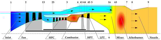
Figure 1.
Schematic diagram of the turbofan engine. Note: Arrows denote the direction of the engine flow path; colors reflect temperature variation (the redder the color, the higher the temperature); numbers represent the definitions of engine sections.
Under steady-state operating conditions, the engine performance parameters must simultaneously satisfy two fundamental physical constraints: the mass flow continuity equations and the static pressure balance equation. In addition, the steady-state process must also ensure power balance between the high-pressure (HP) and low-pressure (LP) rotor shafts. Accordingly, the steady-state co-working equation sets required to be solved for the real-time turbofan engine model are expressed as follows:
where represents the residuals of the equilibrium equations.
Under dynamic operating conditions, due to the power imbalance between the HP and LP rotor shafts, the rotor kinetic equations must be incorporated into the system to enable dynamic updates of the rotational speed parameters. Specifically, the last two equations in Equation (1) are replaced by rotor dynamic equations, resulting in the dynamic co-working equation set of the turbofan engine real-time model, as given by
The numerical solution process of the engine dynamic real-time model follows the following key steps: First, the characteristic pressure ratio parameters of the fan, HPC, HPT, and LPT () are selected as initial guess variables for the iterative solution. Subsequently, the N-R method is employed to simultaneously solve the dynamic co-working equation sets. During the iteration process, model convergence is evaluated by monitoring the residuals of the balance equations, and the engine rotor shaft speeds are updated according to the residual shaft power derived from the rotor dynamic equations ().
However, the real-time calculation performance of the engine model directly affects the response speed of the control system and, consequently, flight safety. Existing engine models often struggle to meet real-time requirements due to their high computational burden and strong nonlinear coupling. To address this issue, three methods are proposed in this paper to enhance the real-time calculation efficiency of the onboard model, based on the established engine performance model. The procedures of these methods are illustrated in Figure 2.
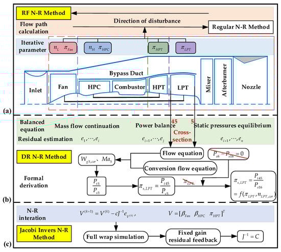
Figure 2.
Framework of the proposed methods: (a) reverse flow (RF N-R) method; (b) dimensionality reduction (DR N-R) method for equations; and (c) constant Jacobian matrix inversion (Jacobi Invers N-R) method. Note: Arrows denote the formula derivation process; red backslashes represent the removed items after formula dimensionality reduction; different colors dash frames in different colors indicate distinct iterative regions.
The regular N-R method is widely adopted in engine dynamic performance modeling, and its calculation reliability and simulation accuracy have been extensively validated in engineering applications. Therefore, the regular N–R method is selected as the benchmark for performance comparison with the proposed approaches.
3. Reverse Flow Method Constructs the Jacobian Matrix
When applying the N–R method to solve the nonlinear equation system of a turbofan engine CLM, the Jacobian matrix plays a critical role in guiding the correction of the initial guess variables during the iterative process. However, the construction of the Jacobian matrix typically requires sequential perturbation of all initial guess variables, and each perturbation necessitates a complete flow path calculation for all engine components, resulting in considerable computational cost.
This section uses a calculation method for constructing the Jacobian matrix based on the inverse flow path method, focusing on the perturbation order of initial guess variables in the CLM of the turbofan engine and the flow path calculation flags.
In the CLM calculation process, to ensure the continuity of thermodynamic variables such as temperature and pressure between adjacent components, the calculation of a single engine component is typically performed along the physical flow direction. That is, the upstream inlet component is calculated first, followed sequentially by downstream components, with the exhaust nozzle computed last. Accordingly, during Jacobian matrix construction, calculation simplifications can be achieved by exploiting the predefined calculation sequence of the engine model, as illustrated in Figure 3.
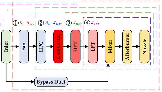
Figure 3.
Influence areas of flow path calculations corresponding to different initial guess variables. Note: Numbers denote the iterative areas, different colors represent separate areas.
Different initial guess variables exert distinct influence ranges on the engine flow path calculations. Specifically, the initial guess variables of the LP rotor shaft speed and fan pressure ratio mainly affect flow path calculation area 1, which is located downstream of the fan. The initial guess variables of the HP rotor shaft speed and HPC pressure ratio primarily influence flow path calculation area 2 downstream of the compressor. The initial guess value of the HPT pressure drop ratio mainly affects flow path calculation area 3 after the HPT, whereas the initial guess value of the LPT pressure drop ratio predominantly affects flow path calculation area 4 after the LPT.
When constructing the Jacobian matrix, the influence areas of each initial guess variable can be identified based on the flow path structure. When perturbing a specific initial guess value, there is no need to recompute component models outside its corresponding influence area, thereby significantly improving the calculation efficiency of the engine model. The forward finite-difference method is commonly adopted to evaluate the partial derivatives of the Jacobian matrix, as expressed in Equation (3).
During the steady-state performance solution process of the engine model, assume that the perturbation sequence of the initial guess variables is denoted as . In the first flow path calculation, the residuals of the equilibrium equations, denoted as , are obtained using the undisturbed initial guess variables. In the second flow path calculation, the LP rotor shaft speed is perturbed, resulting in updated residuals , while the gas path parameters of all components within flow path calculation area 1 are correspondingly updated.
In the third flow path calculation, the HP rotor shaft speed is perturbed. Although the flow path area directly affected by does not include the fan or bypass duct components, the gas path parameters of these upstream components have already been updated during the previous LP shaft speed perturbation. Consequently, it becomes necessary to restore the gas path parameters of the affected components to their pre-perturbation states and to recompute the fan and bypass duct components. As a result, the flow path area that still requires recalculation remains area 1, rather than being limited to area 2. Therefore, this perturbation sequence fails to reduce the overall computational effort of the engine model.
To address this issue, during steady-state performance calculations, the initial guess variables are perturbed in the reverse order of the engine flow direction, following the sequence , when evaluating the elements of the Jacobian matrix. Similarly, during dynamic performance calculations, the perturbation sequence of the initial guess variables should be arranged as . Table 1 and Table 2 summarize the perturbation sequences of the initial guess variables and the corresponding flow path calculation flags for steady-state and dynamic performance calculations.

Table 1.
Flow path calculation flags for Jacobian matrix construction in the steady-state process.
Table 2.
Flow path calculation flags for Jacobian matrix construction in the dynamic process.
Compared with the steady-state performance calculation, a larger proportion of engine components can be excluded from recomputation during the dynamic performance calculation. As a result, the real-time calculation performance of the engine dynamic model is significantly enhanced.
4. Dimensionality Reduction of Working Equation Sets
Within an acceptable range of simulation errors, the dimensionality of the nonlinear equations can be simplified by reducing the number of initial guess variables and the number of coupled working equations. This significantly enhances the real-time performance of iterative calculations for the engine dynamic performance model.
We assume that the inlet guide vane throat of the turbine component is in a critical state, that is, the equivalent gas flow rate through the turbine remains constant. For different initial guess variables of the turbine pressure drop ratio, since the total temperature and total pressure upstream of the turbine are identical, the mass flow rate of the gas entering the turbine calculated according to the flow formula is also the same. Therefore, the role of the turbine pressure drop ratio in the process of solving the collaborative working equations is to match the flow balance constraints of the downstream components of the turbine. Using this matching principle, by reducing the LPT pressure drop ratio in the initial guess value set of the engine and removing the corresponding static pressure balance equation , dimensionality reduction in the collaborative working equation set at the component level is achieved.
The flow equations for the inlet and outlet of the LPT are presented in Equation (4). Based on the principle of similarity, the converted flow equations for the inlet and outlet of the LPT are shown in Equation (5).
where is the gas flow function that depends on the Mach number , and is the amplification factor, which is related to the gas adiabatic index and gas constant . are as shown in Equation (6).
Dividing the two equations in (4) yields the relationship of air flow variation at the inlet and outlet of the LPT, as shown in Equation (7).
Based on the relationship between the inlet and outlet air–gas flow rates of the LPT, component characteristics, and the hypothesis of flow rate balance at the inlet and outlet, the corrected gas flow rate relationship at the inlet and outlet of the LPT can be derived, as shown in Equation (8).
where is the LPT pressure drop ratio, and is the LPT relative corrected speed, as shown in Equation (9).
From the corrected gas flow rate relationship between the inlet and outlet of the LPT in Equation (8) and the relationship among the pressure drop ratio, corrected gas flow rate, and inlet corrected rotor shaft speed in the characteristic diagram in Equation (10), the outlet corrected gas flow characteristics of the LPT can be obtained, as shown in Equation (11).
The characteristics of the Mach number at the LPT outlet can be calculated using Equation (11) and the corrected gas flow rate formula, Equation (5), for the LPT outlet, as shown in Equation (12).
The total and static pressure relationship of the LPT at the outlet can be calculated using the total and static pressure formula in Equation (13).
From Equation (13), the relationship between the total pressure at the inlet of the LPT and the static pressure at the outlet can be derived as Equation (14). Then, the pressure drop ratio used for interpolation in the LPT characteristic graph is modified to be represented by the pressure drop ratio , which is the total pressure at the LPT inlet divided by the static pressure at the LPT outlet.
In the CLM of the turbofan engine, the static pressure at the inner nozzle exit section is used to substitute for the LPT exit static pressure . The static pressure balance equation presented in Equation (1) depicts the equality of the static pressure at the outer nozzle exit and that at the inner nozzle exit. Therefore, the outer nozzle exit static pressure can be employed to replace the LPT exit static pressure, leading to the LPT characteristics represented by Equation (15).
Based on the LPT characteristics shown in Equation (15), the LPT characteristic curves of the pressure drop ratio–corrected gas flow rates and total static pressure drop ratio–corrected gas flow rates can be plotted, as shown in Figure 4.
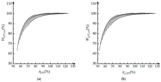
Figure 4.
LPT characteristic diagram: (a) pressure drop ratio–corrected gas flow rates of LPT characteristic curve; (b) total static pressure drop ratio–corrected gas flow rates of LPT characteristic curve.
Therefore, in the flow path calculation, the LPT component can be computed using Equation (15), which naturally satisfies the static pressure balance equation of the engine and does not require additional initial guess variables for the LPT pressure drop ratio. Therefore, the steady-state performance calculation model of the engine requires five initial guess variables, , while the dynamic performance calculation requires three initial guess variables, . When using the N-R method to solve the nonlinear equations, one gas flow path calculation can be reduced, thereby improving the real-time performance calculation efficiency of the engine model.
5. Balancing Technique of the Jacobian Matrix Inverse
The N-R method utilizes the residuals of the dynamic collaboration equations to acquire the partial derivative information of the initial guess variables. That is, the Jacobian matrix is continuously adjusted for the initial guess variables until the collaborative set of equations converges iteratively.
For the turbofan engine CLM, this section investigates the variation patterns of the elements of the inverse Jacobian matrix under different operating conditions of the engine and proposes a balancing technique based on constant Jacobian matrix inversion.
The elements of the inverse of the Jacobian matrix are derived from corrections to the initial guess variables during the iteration process. However, during the characteristic curve interpolation process, there may be instances where the characteristic curve exhibits non-monotonic behavior in the upper left quadrant of the characteristic map of the compression components’ air flow rates and pressure ratio [36]. In such cases, the compressor operating points fall near the unstable boundary, which can result in the calculation of different air flow rates at the same pressure ratio through characteristic map interpolation. This non-monotonicity is clearly detrimental to the iterative solution, affecting the model’s computational accuracy and stability [37].
The value interpolation method for compression components is a commonly used approach to effectively resolve this issue. Although the value does not have obvious physical significance, it can be used to describe the relative position of the operating point in the characteristic map, as illustrated in Figure 5, thus facilitating model convergence.
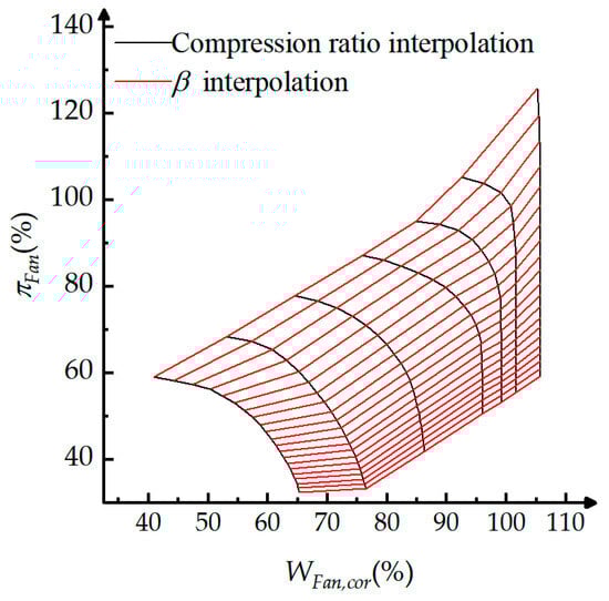
Figure 5.
interpolation of the fan characteristic curves.
In order to further reduce the initial guess variables for the fan and LPT, it is necessary to update with more balancing equation errors. By combining the value interpolation method with the dimensionality reduction method for equations, the pressure ratio drop of the LPT and the static pressure balancing equation are simplified, resulting in a dynamic engine model that contains only three initial guess variables, , and analysis of the inverse elements of the Jacobian matrix is performed.
As shown in Figure 6, forty typical flight states within the full flight envelope are selected to analyze the inverse elements of the Jacobian matrix. The selected typical flight states can fully cover the flight envelope formed by altitude () and Mach number (Ma) (Figure 6a) and can also adequately represent the flight envelope formed by the total temperature and total pressure in the engine inlet section (Figure 6b).The specific altitudes and Mach numbers of forty typical flight states are shown in Table 3.
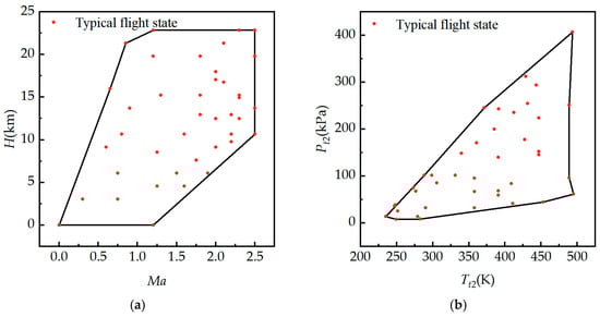
Figure 6.
Full flight envelope diagram: (a) altitude and Mach number flight envelope; (b) total pressure and total temperature flight envelope.
Table 3.
Forty typical flight states corresponding to labels, altitudes, and Mach numbers.
In the dynamic performance solution process, even when the HP and LP rotor shaft speeds are the same, the engine’s characteristics can vary under different fuel flow rates. Therefore, based on the engine’s steady state, by fixing the state variables of the HP and LP rotor shaft speeds of the engine and changing the fuel flow rate, we can simulate a broader range of the engine’s dynamic characteristics. This enables us to obtain the variation in the inverse Jacobian matrix elements under different dynamic conditions.
Based on the forty flight states listed in Table 3, for each flight condition, multiple operating points where the LP rotor shaft speed ranges from 70% to 100% were considered. A quasi-steady-state point was selected every 5%, resulting in a total of seven state points. For each state point, ten different engine working states were selected by adjusting the steady-state fuel flow rate up and down by ±40%. This provides sufficient dynamic excitation for the inverse Jacobian matrix elements. The total average value of the elements of the inverse Jacobian matrix from all seven state points, obtained by averaging the values across seventy states, represents the result of the elements of the inverse Jacobian matrix for that flight state point. Applying the aforementioned method, the Jacobian inverse matrix elements for forty flight states were obtained. Figure 7 shows the variation in the average values of the elements of the inverse Jacobian matrix across forty flight state points.
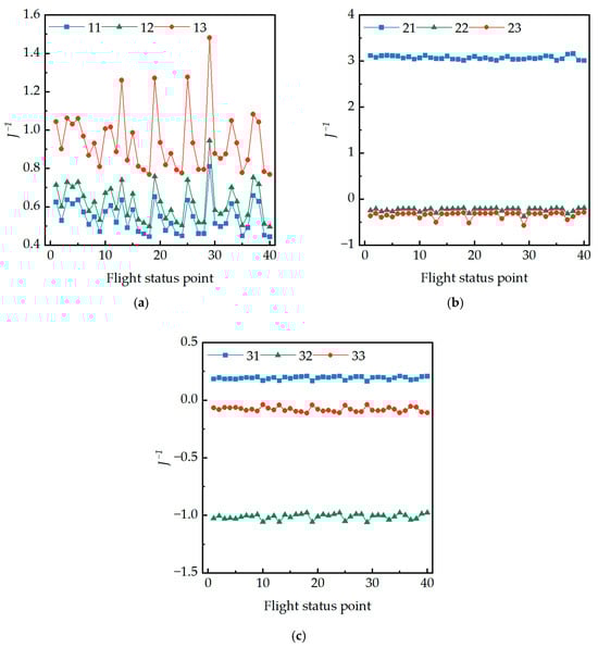
Figure 7.
Variation regularity of average values of each element in the inverse Jacobian matrix under typical flight states for full flight envelope: (a) average value of the elements in the first row of the Jacobian matrix inverse; (b) average value of the elements in the second row of the Jacobian matrix inverse; and (c) average value of the elements in the third row of the Jacobian matrix inverse.
From Figure 7, it can be observed that the average values of the elements in the second and third rows of the inverse Jacobian matrix exhibit little variation within the bounding envelope. Therefore, fixed-gain residual feedback can be employed to correct the initial estimates of values and .
Regarding the elements in the first row of the inverse Jacobian matrix, although their average values fluctuate within the bounding envelope, fixed-gain residuals can still be selected to correct the initial value estimate . Since the magnitudes of the three elements are comparable, three fixed-gain residuals are ultimately chosen for the correction of the initial value estimate . The current correction for the initial value estimates is provided by Equation (16).
In the formula, is the initial guess value matrix, is the damping coefficient, and is the fixed inverse of the Jacobian matrix, as shown in Equation (17).
The inverse of the regular Jacobian matrix is summarized from empirical rules derived from statistical analysis of the variation trends of the inverse elements of the Jacobian matrix under forty typical flight conditions within the envelope.
6. Simulation and Analysis
To systematically verify the reliability, engineering feasibility, and robustness of the three proposed methods, this section establishes a multi-operating-condition comparative validation framework, conducting a quantitative comparative analysis between the three proposed methods and the regular N-R method in terms of real-time calculation accuracy and dynamic performance.
The validation experiments are divided into two core dimensions based on operating condition complexity and practical applicability: First, baseline validation is carried out within the rated operating conditions of the aero-engine—under this operating condition, all core components of the engine operate in a state of steady equilibrium, and both the load characteristics and environmental parameters are strictly consistent with the design baseline variables. This setup effectively eliminates extreme interference factors, enabling an objective evaluation of the method’s basic performance and stability under ideal operating conditions. Furthermore, to replicate the dynamic performance degradation characteristics of aero-engines during actual service, which are induced by factors such as component wear, fouling, and erosion, the validation scenario is extended to more stringent off-design operating conditions for supplementary verification.
In the real-time validation of turbofan engine performance simulation, the nozzle area undergoes continuous variation throughout the process. Figure 8 depicts the variation in the nozzle throat area with HP rotor shaft speed under open-loop control conditions.
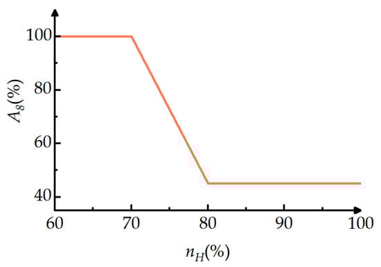
Figure 8.
Open-loop control law of the nozzle throat area A8 with respect to HP rotor shaft speed.
6.1. Reverse Flow Method
6.1.1. Rated Operating Conditions
This section aims to validate the feasibility of the RF N-R method under rated operating conditions. To this end, we compare the RF N-R method with the regular N-R method, focusing on the accuracy and calculation time of steady-state, regular transient, and small-step transient calculations, in order to assess the method’s effectiveness and applicability.
Figure 9 and Figure 10 present a comparison of the engine’s steady-state and regular transient performance simulation results using the regular N-R method and the RF N-R method. Among them, Figure 9a and Figure 10a, respectively, show the fuel changes during steady-state and regular transient acceleration processes, while the other figures depict changes in engine performance parameters.
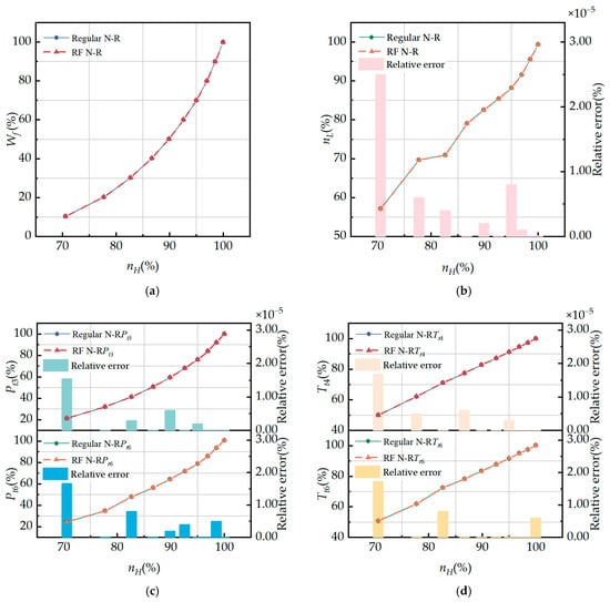
Figure 9.
Comparison of regular N-R method and RF N-R method steady-state performance simulation: (a) fuel flow rate; (b) LP and HP rotor shaft speeds; (c) HPC and internal duct outlet total pressure; and (d) combustion and internal duct outlet total temperature.
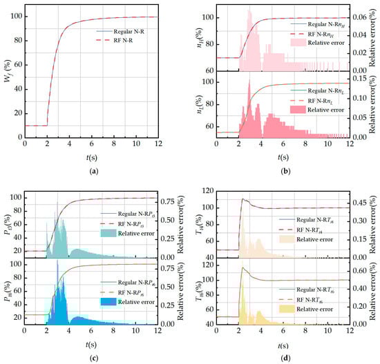
Figure 10.
Comparison of regular N-R method and RF N-R method regular transient performance simulation: (a) fuel flow rate; (b) LP and HP rotor shaft speeds; (c) HPC and internal duct outlet total pressure; and (d) combustion and internal duct outlet total temperature.
To further verify the feasibility of this method, small-step transient performance simulations of the engine are performed. As shown in Figure 11, a direct comparison is drawn between the small-step transient simulation results obtained via the regular N-R method and the RF N-R method. In detail, Figure 11a characterizes the fuel supply variation during the small-step transient process, while other subplots exhibit the dynamic responses of critical engine performance metrics. Notably, the MRE associated with the core engine gas path parameter calculations in the transient processes is limited to 1.6%, well within the acceptable range for engineering practice.
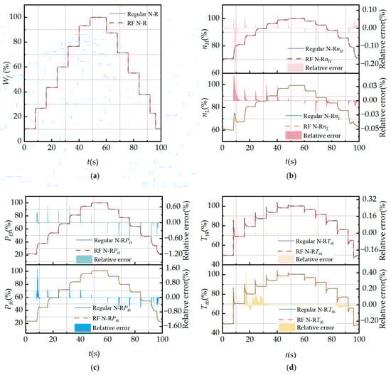
Figure 11.
Comparison of regular N-R method and RF N-R method small-step transient performance simulation: (a) fuel flow rate; (b) LP and HP rotor shaft speeds; (c) HPC and internal duct outlet total pressure; and (d) combustion and internal duct outlet total temperature.
The performance tests are conducted on a computer equipped with an 11th-generation Intel Core i5-11400 processor (manufactured by Intel Corporation, headquartered in Santa Clara, CA, USA; clock speed: 2.60 GHz) under Sea-Level International Standard Atmosphere conditions (), covering steady-state processes, regular transient processes from the idle state to the mid-state (as shown in Figure 9 and Figure 10), and small-step transient processes cycling from the idle state to the mid-state and back to the idle state (as shown in Figure 11), with each process repeated 10,000 times to ensure test reliability.
Figure 12 compares the number of steady-state, regular transient, and small-step transient simulation iterations between the two methods. The specific calculation time comparison is presented in Table 4. It can be noted that, compared to the steady-state performance simulation process, the ratio of components that do not require calculation to those that do is higher during the engine transient performance simulation process. Therefore, the proposed RF N-R method significantly reduces the number of dynamic model iterations and enhances the real-time performance of engine transient calculations. During the transient process, the real-time performance is optimized to the greatest extent, with the improvement magnitude reaching as high as 33.9%.
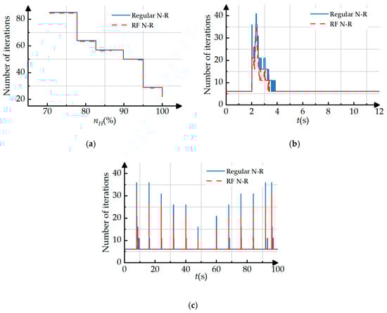
Figure 12.
Comparison of regular N-R method and RF N-R method number of iterations: (a) steady-state simulation number of iterations; (b) regular transient simulation number of iterations; and (c) small-step transient simulation number of iterations.
Table 4.
Comparison of calculation time for steady-state, regular transient, and small-step transient performance simulation between regular N-R method and RF N-R method.
6.1.2. Off-Design Operating Conditions
To validate the feasibility of the RF N-R method under off-design operating conditions, we first focus on the engine performance degradation process, clearly defining the degradation levels. Subsequently, we compare the RF N-R method with the regular N-R method, with a particular emphasis on the accuracy and calculation time of small-step transient calculations, to evaluate the method’s applicability under off-design operating conditions.
This study focuses on the extreme scenario of aero-engine performance degradation, whose core characteristic is manifested as the regular deviation of key parameters in the component performance map. Guided by the thermodynamic principles and component degradation mechanisms of aero-engines, the constraint conditions are explicitly defined as follows: as gas compression components, the fan and HPC exhibit a monotonic decreasing trend in the flow rate with the occurrence of degradation phenomena such as wear and fouling; as power output components, the HPT and LPT experience a monotonic increase in the flow rate due to the change in flow capacity, which is induced by factors including blade erosion and clearance enlargement; and the adiabatic efficiency of all core components decreases continuously with performance degradation, reflecting the loss of energy conversion efficiency [38].
Within this constraint framework, combined with the typical fault modes and degradation laws of aero-engines, the degradation levels of health parameters are classified into three categories, as presented in Table 5, namely, slight, intermediate, and extreme degradation.
Table 5.
Classification of degradation levels of core component health parameters.
To accurately reproduce the real operating conditions associated with engine performance degradation, the degradation characteristic parameters of different severity levels listed in Table 5 are injected into the rotating components of the engine under boundary conditions identical to those adopted in the small-step transient performance simulations, including the fuel input scheduling, initial state settings, and environmental parameters. Based on this configuration, multi-scenario simulation models covering slight, intermediate, and extreme degradation levels are established.
Figure 13 provides an intuitive illustration of the distribution characteristics of the MRE of six key engine performance parameters obtained using both the regular N–R method and the RF N–R method under the three aforementioned degradation levels, with the results visualized in the form of a quantitative heatmap.
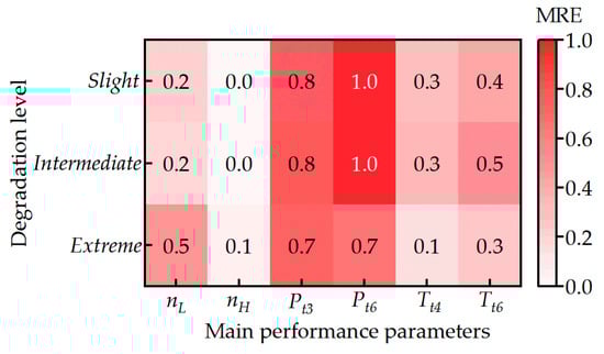
Figure 13.
Heatmap of MRE of performance parameters for regular N-R method and RF N-R method under three degradation levels.
Analysis of the numerical distribution patterns in the heatmap reveals that the MRE values exhibit no significant correlation with the aggravation of degradation levels. This finding confirms that the RF N-R method can maintain stable parameter estimation accuracy even under extreme degradation conditions, demonstrating excellent robustness. Further quantitative statistical results indicate that the MRE of the RF N-R method is consistently and strictly constrained within 1.0%. This fully verifies the high-precision estimation capability of the method in engine performance degradation scenarios, providing reliable data support for its potential engineering applications.
To systematically evaluate the real-time performance of the proposed method, 1000 independent repeated simulation experiments are conducted under both the regular N-R method and the RF N-R method frameworks. The average computational time per simulation for the two methods is statistically analyzed and compared, with the results presented in Table 6. Quantitative analysis indicates that compared with the non-degraded operating condition, the real-time performance improvement margin of the RF N-R method only exhibits slight attenuation under degraded operating conditions, and the attenuation degree is strictly constrained within 6%, while maintaining a significant calculation efficiency advantage.
Table 6.
Comparison of simulation calculation time for small-step transient performance between regular N-R method and RF N-R method under three degradation levels.
In conclusion, regardless of whether the aero-engine is in a healthy state or subject to performance degradation of varying degrees, the RF N-R method can significantly improve the real-time calculation efficiency of engine performance simulation while ensuring the stable and controllable accuracy of parameter estimation, which fully verifies the engineering practicability and operating condition adaptability of this method.
6.2. Dimensionality Reduction Method for Equations
6.2.1. Rated Operating Conditions
This section aims to evaluate the feasibility of the DR N-R method under rated operating conditions. To this end, we compare the DR N-R method with the regular N-R method, focusing on the accuracy and calculation time of steady-state, regular transient, and small-step transient calculations, in order to assess the method’s effectiveness and applicability.
Figure 14 and Figure 15 present a comparison of the steady-state and regular transient performance simulations of the engine using the regular N-R and DR N-R methods. Among them, Figure 14a and Figure 15a, respectively, show the fuel changes during steady-state and regular transient processes, while the other figures depict changes in engine performance parameters. Owing to the utilization of the interpolation characteristic diagram of the total pressure at the LPT inlet and the static pressure ratio at the outlet section, errors occur when compared with the regular N-R method. The steady-state performance calculation MRE of the engine’s main gas path parameters is within 0.6%. The regular transient performance calculation MRE of the engine’s main gas path parameters is within 1.4%, which can satisfy the engineering usage requirements.
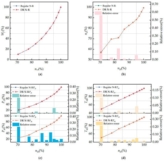
Figure 14.
Comparison of regular N-R method and DR N-R method steady-state performance simulation: (a) fuel flow rate; (b) LP and HP rotor shaft speeds; (c) HPC and internal duct outlet total pressure; and (d) combustion and internal duct outlet total temperature.
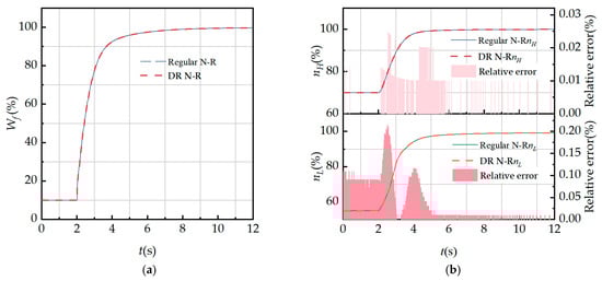
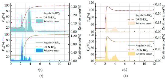
Figure 15.
Comparison of regular N-R method and DR N-R method regular transient performance simulation: (a) fuel flow rate; (b) LP and HP rotor shaft speeds; (c) HPC and internal duct outlet total pressure; and (d) combustion and internal duct outlet total temperature.
Given the concerns associated with the elimination of the corresponding static pressure balance equation, small-step transient performance simulations are further conducted to validate the feasibility of the proposed method. Figure 16 presents a comparative analysis of engine small-step transient performance predictions derived from the regular N-R method and the DR N-R method. Specifically, Figure 16a illustrates the variation in the fuel supply rate throughout the small-step transient process, whereas the remaining subfigures depict the dynamic evolutions of key engine performance parameters.
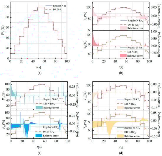
Figure 16.
Comparison of regular N-R method and DR N-R method small-step transient performance simulation: (a) fuel flow rate; (b) LP and HP rotor shaft speeds; (c) HPC and internal duct outlet total pressure; and (d) combustion and internal duct outlet total temperature.
Notably, the acceleration and deceleration processes encompass operating points under low-speed conditions, where the LPT operates in a subcritical state. As clearly observed from the figures, the relative errors at these low-condition points are comparatively large. Thus, the removal of the static pressure balance equation exerts a non-negligible influence on the model calculations at low-condition operating points. Nevertheless, quantitative results indicate that the MRE of the predicted core engine gas path parameters during small-step transient operations is within 1%, which satisfies the stringent requirements of engineering applications.
To further demonstrate the performance of the DR N-R method, the real-time performance of the following processes was tested on a computer equipped with an 11th-generation Intel Core i5-11400 processor (manufactured by Intel Corporation, headquartered in Santa Clara, CA, USA; clock speed: 2.60 GHz), under Sea-Level International Standard Atmosphere conditions (), by running the process 10,000 times: the steady-state and regular transient acceleration processes from the idle state to the mid-state (as shown in Figure 14 and Figure 15) and the small-step transient acceleration and deceleration processes from the idle state to the mid-state and back to the idle state (as shown in Figure 16).
Figure 17 compares the number of steady-state, regular transient, and small-step transient simulation iterations between the two methods. The specific calculation time comparison is shown in Table 7. It can be observed that, since the DR N-R method is utilized in each flow path calculation, the number of model iterations will decrease, thereby improving the real-time performance of engine dynamic calculations. During the transient process, the real-time performance is optimized to the greatest extent, with the improvement magnitude reaching as high as 36.6%.
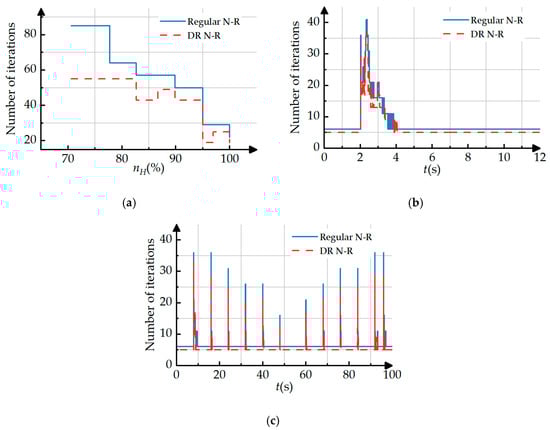
Figure 17.
Comparison of regular N-R method and DR N-R method number of iterations: (a) steady-state simulation number of iterations; (b) regular transient simulation number of iterations; and (c) small-step transient simulation number of iterations.
Table 7.
Comparison of calculation time for steady-state, regular transient, and small-step transient performance simulation between the regular N-R method and the DR N-R method.
6.2.2. Off-Design Operating Conditions
To verify the effectiveness of the DR N-R method, this section conducts simulation tests under off-design operating conditions, with a focus on analyzing the calculation time reduction ratio and relative error of small-step transient calculations. To investigate the applicability and accuracy characteristics of the DR N-R method under engine performance degradation scenarios, the degradation characteristic parameters of different levels listed in Table 5 of Section 6.1.2 were injected into each rotating component of the engine under the identical fuel supply strategy and boundary constraints adopted in the aforementioned small-step transient performance simulation, thereby constructing an engine performance degradation simulation model covering multiple typical operating conditions.
Figure 18 systematically presents the distribution characteristics of the MRE of the regular N-R method and the DR N-R method for six core performance parameters of the engine under three degradation levels in the form of a quantitative heatmap. Quantitative analysis of the evolution law of error values in the heatmap reveals that the MRE exhibits a significant positive correlation with the aggravation of degradation levels. Critically, under extreme degradation conditions, the parameter estimation accuracy of the DR N-R method deteriorates remarkably, with its peak MRE reaching as high as 23%—far exceeding the 5% error tolerance threshold in engineering applications and thus failing to meet the requirements for precise estimation of performance parameters.
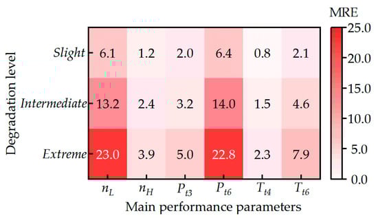
Figure 18.
Heatmap of MRE of main performance parameters for regular N-R method and DR N-R method under three degradation levels.
To reveal the intrinsic mechanism underlying the aforementioned error deterioration phenomenon, an in-depth analysis was conducted on the core flow path aerodynamic characteristics during the engine degradation process. The results indicate that in the course of engine performance degradation, the Mach number of the air flow in the throat section of the inlet guide vane of the LPT can no longer reach 1.0, meaning that the air flow in this section has transformed from the critical state under design conditions to a subcritical state. However, the establishment of the DR N-R method is based on an explicit premise: the throat section of the inlet guide vane of the turbine component operates under critical flow conditions. This assumption constitutes the core basis for achieving equation dimensionality reduction and improving solution efficiency. When the throat section of the LPT inlet guide vane enters a subcritical state, the core premise of the DR N-R method is no longer valid. Consequently, the static pressure equilibrium equation eliminated based on this assumption becomes a key constraint equation affecting the matching between the flow field and performance parameters under subcritical flow conditions.
One thousand independent repeated simulation experiments are conducted for each of the two methods, and the average calculation time per simulation is summarized, with the specific data presented in Table 8. The results demonstrate that the DR N-R method exhibits a certain advantage in computational efficiency compared with the regular N-R method, with a time reduction ranging from 11.0% to 13.0%, which indicates a noticeable improvement in real-time performance.
Table 8.
Comparison of simulation calculation time for small-step transient performance between regular N-R method and DR N-R method under three degradation levels.
In summary, under off-design operating conditions induced by degradation, especially deep degradation conditions, the simplification of removing the static pressure equilibrium equation exerts a non-negligible negative impact on the calculation accuracy of the model, ultimately leading to a significant expansion of parameter estimation errors. It can be concluded that within the full operating condition range of engine performance degradation, although the DR N-R method can improve the real-time performance of engine performance simulation to a certain extent, its parameter estimation accuracy decreases sharply with the deepening of the degradation degree, making it difficult to meet the engineering application requirements of high-precision simulation.
6.3. Constant Jacobian Matrix Inversion Method
6.3.1. Rated Operating Conditions
Based on the inverse of the regular Jacobian matrix, a dynamic performance simulation of the engine for the 34 min flight trajectory [39] shown in Figure 19 was conducted to test the real-time performance and accuracy of the model using the Jacobi Invers N-R method.
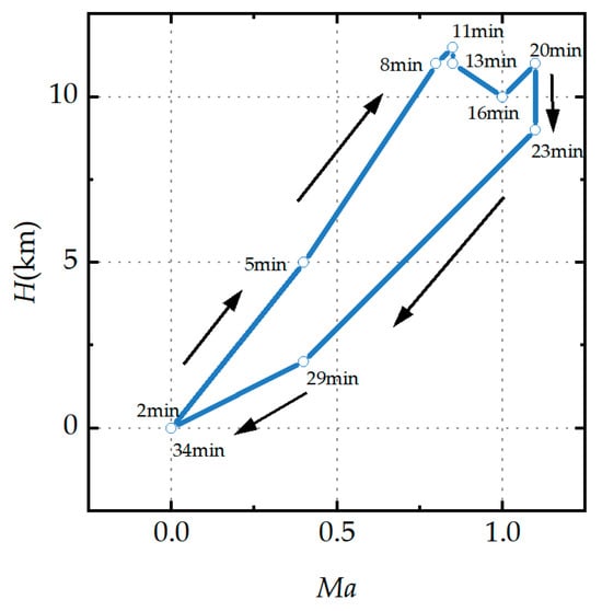
Figure 19.
Dynamic testing flight trajectory. Note: The arrows in the figure indicate the direction of the flight path.
Figure 20 shows a comparison of the engine’s dynamic performance simulation using the regular N-R method and the Jacobi Invers N-R method. Among them, Figure 20a shows the fuel changes during the flight process, while the other figures depict changes in engine performance parameters. The MRE in the main engine parameters is within 1.6%, which meets the accuracy requirements for engine model calculations.
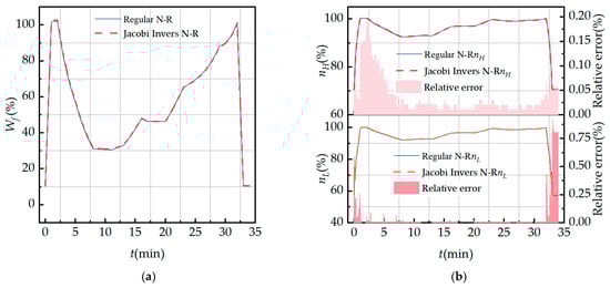
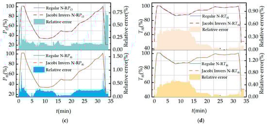
Figure 20.
Comparison of regular N-R method and Jacobi Invers N-R method dynamic performance simulation: (a) fuel flow rate; (b) LP and HP rotor shaft speeds; (c) HPC and internal duct outlet total pressure; and (d) combustion and internal duct outlet total temperature.
The performance of the Jacobi Invers N-R method is evidenced using a computer equipped with an 11th-generation Intel Core i5-11400 processor (manufactured by Intel Corporation, headquartered in Santa Clara, CA, USA; clock speed: 2.60 GHz), under Sea-Level International Standard Atmosphere conditions (), based on the flight process shown in Figure 19, with the process repeated 100 times to ensure test reliability. Figure 21 compares the number of iterations between the two methods. The specific computational time comparison is shown in Table 9. It can be observed that after incorporating the DR N-R method, the Jacobi Invers N-R method significantly reduces the number of iterations, with the calculation time decreasing by 50.9%, which markedly improves the real-time performance of engine dynamic calculations.
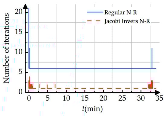
Figure 21.
Comparison of regular N-R method and Jacobi Invers N-R method number of iterations.
Table 9.
Comparison of calculation time for dynamic performance simulation between regular N-R method and Jacobi Invers N-R method.
6.3.2. Off-Design Operating Conditions
To systematically evaluate the applicability and parameter estimation accuracy of the Jacobi Invers N-R method under aircraft engine performance degradation conditions, a comparative simulation study is conducted in this work under identical fuel scheduling, flight condition variations, and boundary constraints corresponding to the previously described 34-min flight trajectory. According to the degradation characteristic parameters of different severity levels listed in Table 5 of Section 6.1.2, three performance degradations are injected into the efficiency and flow capacity parameters of the engine rotating components. In this manner, an engine degradation simulation model covering multiple representative operating conditions and capable of capturing the evolution characteristics of performance deterioration is established.
Figure 22 presents a quantitative comparison, in the form of a heatmap, of the MRE distributions of six key engine performance parameters obtained using the regular N–R method and the Jacobi Invers N-R method under the three degradation levels. Quantitative analysis of the error magnitudes and their variation trends with increasing degradation severity indicates that the MRE increases significantly as engine degradation intensifies, demonstrating that performance degradation generally deteriorates the parameter estimation accuracy of the Jacobi Invers N-R method. In particular, under extreme degradation conditions, the estimation accuracy of the Jacobi Invers N-R method degrades markedly, with the peak MRE reaching approximately 17%, which substantially exceeds the commonly accepted 5% error tolerance in engineering applications and therefore fails to meet the requirements for accurate engine performance parameter estimation and health monitoring.

Figure 22.
Heatmap of MRE of main performance parameters for regular N-R method and Jacobi Invers N-R method under three degradation levels.
To further elucidate the underlying mechanism responsible for the observed accuracy degradation, an in-depth analysis is performed on the variations in the aerodynamic and thermodynamic characteristics of the core flow path during the engine degradation process. The results indicate that, as component efficiencies decrease and flow characteristics deteriorate, the flow matching relationships and energy coupling among engine components undergo significant changes, leading to a pronounced increase in system nonlinearity. Under such conditions, the Jacobi Invers N-R method, which relies on a fixed Jacobian matrix to approximate local system sensitivities, is unable to accurately capture the continuously evolving nonlinear mapping between state values and performance parameters. Consequently, the direction and magnitude of the iterative corrections gradually deviate from the true optimal solution.
For each method, 100 independent repeated simulation runs are conducted, and the average calculation time per simulation is recorded. The corresponding results are summarized in Table 10. The results indicate that the Jacobi Invers N-R method exhibits higher calculation efficiency than the regular N-R method, with a calculation time reduction of approximately 48–51%, demonstrating a certain degree of real-time performance improvement.
Table 10.
Comparison of calculation time for dynamic performance simulation between regular N-R method and Jacobi Invers N-R method under three degradation levels.
Therefore, although the Jacobi Invers N-R method offers a noticeable advantage in calculation efficiency, its applicability is inherently constrained to weakly nonlinear operating conditions. When the engine operates under moderate-to-severe performance degradation, the system nonlinearity increases significantly, making it difficult for this method to simultaneously maintain high calculation efficiency and estimation accuracy, thereby limiting its engineering applicability.
7. Conclusions
This paper conducts a systematic study on the real-time optimization of dynamic models for aircraft engines. Taking a specific twin-spool mixed-exhaust turbofan engine as the research object, three innovative computational methods aiming to improve real-time performance are proposed. The main research findings are as follows:
- (1)
- The RF N-R method is proposed: By constructing the Jacobian matrix along the inverse flow path, it avoids redundant calculations and reduces iteration times. Compared with the regular N-R method, the steady-state, regular transient, and small-step transient performance calculation time is reduced by 27.6%, 33.9%, and 30.8%, respectively, and the MRE of major parameters is within 1.6%.
- (2)
- In terms of solving the nonlinear coupled equations, dimension reduction optimization of the equations is achieved based on aerodynamic thermodynamics principles. This reduces one complete flow path calculation and enhances real-time performance. Compared to the regular N-R method, the steady-state, regular transient, and small-step transient performance calculation time is reduced by 20.1%, 11.4%, and 36.6%, respectively, and the MRE of major parameters is within 1.4%.
- (3)
- The Jacobi Invers N-R method is proposed: Utilizing the property of small changes in the Jacobian inverse elements within the full flight envelope, fixed gains are substituted to simplify dynamic performance calculations. Compared with the regular N-R method, the dynamic performance simulation process within the full flight envelope can reduce the calculation time by 50.9%, while the MRE of major parameters is within 1.6%.
In summary, compared with current state-of-the-art methods, the proposed approaches exhibit distinct trade-offs in computational demand, implementation complexity, and applicability. The Broyden and quasi-Newton method approaches rely on approximate Jacobian updates and may suffer from reduced robustness under wide-envelope operation and performance degradation, whereas the Jacobi Invers N-R method is computationally efficient but restricted to weakly nonlinear conditions. The DR N-R method decreases online computation at the expense of substantial offline effort and reduced accuracy under off-design and deeply degraded conditions. In contrast, the proposed RF N-R method enhances real-time performance without Jacobian approximation or model simplification while maintaining stable accuracy across the full operating envelope and varying degradation levels, thereby demonstrating superior engineering applicability.
It is worth mentioning that the methods proposed in this paper for enhancing the real-time calculation performance of onboard models are applicable to various types of aircraft engines. In the future, we will apply the real-time enhancement methods proposed in this paper to structurally complex variable cycle engines to further verify the reliability of the methods.
Author Contributions
Conceptualization, W.Z. and J.H.; methodology, L.G.; software, L.G.; validation, W.Z., J.H. and R.W.; formal analysis, L.G.; investigation, W.Z. and R.W.; resources, R.W.; data curation, L.G.; writing—original draft preparation, L.G. and R.W.; visualization, W.Z.; supervision, Y.C.; project administration, W.Z.; funding acquisition, W.Z. and J.H. All authors have read and agreed to the published version of the manuscript.
Funding
This research received no external funding.
Data Availability Statement
Data are contained within the paper.
Conflicts of Interest
Author Rong Wang was employed by the company CH UAV Science & Technology Co., Ltd. The remaining authors declare that the research was conducted in the absence of any commercial or financial relationships that could be construed as a potential conflict of interest.
Abbreviations
| Gas mass flow rate | |
| Pressure | |
| Rotor shaft speed | |
| Current moment | |
| Moment of inertia | |
| Mechanical efficiency | |
| Component power | |
| Pressure ratio | |
| Residual | |
| Mach number | |
| Initial guess value matrix | |
| Damping coefficient | |
| Jacobian matrix | |
| Component operating point auxiliary parameter | |
| Amplification factor | |
| Area | |
| Temperature | |
| Gas adiabatic index | |
| Gas constant | |
| Altitude | |
| RF N-R | Reverse flow |
| MRE | Maximum relative error |
| DR N-R | Dimensionality reduction for equations |
| Jacobi Invers N-R | Constant Jacobian matrix inversion |
| subscript | |
| Gas | |
| Air | |
| Fuel | |
| Combustor fuel | |
| Afterburner fuel | |
| Static | |
| High-pressure rotor shaft | |
| High-pressure turbine | |
| High-pressure compressor | |
| Attachment extraction | |
| Low-pressure rotor shaft | |
| Low-pressure turbine | |
| Total | |
| Corrected | |
References
- Chen, J.; Hu, Z.; Wang, J. Aero-Engine Real-Time Models and Their Applications. Math. Probl. Eng. 2021, 2021, 9917523. [Google Scholar] [CrossRef]
- Chen, Y.; Lu, S.; Chen, Z.; Zhou, W.; Huang, J. Hybrid Onboard Model of High-Flow Dual Variable Cycle Engine Based on Deep Reinforcement Learning. Chin. J. Aeronaut. 2025, 103792. [Google Scholar] [CrossRef]
- Liu, B.; Feng, H.; Xu, M.; Li, M.; Song, Z. An Enhanced Non-Iterative Real-Time Solver via Multilayer Perceptron for on-Board Component-Level Models. Energy 2024, 303, 131826. [Google Scholar] [CrossRef]
- Saravanamuttoo, H.I.H.; Rogers, G.F.C.; Cohen, H. Gas Turbine Theory; Pearson education: London, UK, 2001; pp. 12–25. [Google Scholar]
- Wei, Z.; Zhang, S.; Jafari, S.; Nikolaidis, T. Gas Turbine Aero-Engines Real Time on-Board Modelling: A Review, Research Challenges, and Exploring the Future. Prog. Aerosp. Sci. 2020, 121, 100693. [Google Scholar] [CrossRef]
- Guo, Y.; Teng, J.; Zhou, X.; Zou, Z.; Huang, J.; Lu, F. Real-Time Adaptive Model of Mainstream Parameters for Aircraft Engines Based on OSELM-EKF. Aerosp. Sci. Technol. 2024, 155, 109662. [Google Scholar] [CrossRef]
- Zhang, X.; Zhang, T.; Sheng, H. A Novel Aeroengine Real-Time Model for Active Stability Control: Compressor Instabilities Integration. Aerosp. Sci. Technol. 2024, 145, 108844. [Google Scholar] [CrossRef]
- Volponi, A.; Simon, D.L. Enhanced self tuning on-board real-time model (eSTORM) for aircraft engine performance health tracking. NASA 2008, 2008, 215272. [Google Scholar]
- Tahan, M.; Tsoutsanis, E.; Muhammad, M.; Karim, Z.A. Performance-based health monitoring, diagnostics and prognostics for condition-based maintenance of gas turbines: A review. Appl. Energy 2017, 198, 122–144. [Google Scholar] [CrossRef]
- Konstantinos, M.; Alexiou, A.; Aretakis, N.; Romesis, C. Signatures of compressor and turbine faults in gas turbine performance diagnostics: A review. Energies 2024, 17, 3409. [Google Scholar] [CrossRef]
- Huang, J.; Zhang, T.; Ye, Z.; Zhou, W.; Pan, M. Modern Aviation Power Device Control, 3rd ed.; Aviation Industry Press: Beijing, China, 2018; pp. 38–65. [Google Scholar]
- Cai, C.; Zheng, Q.; Zhang, H. A New Method to Improve the real-time calculation performance of Aero-Engine Component Level Model. Int. J. Aerosp. Eng. 2020, 40, 101–109. [Google Scholar]
- Gazzetta, H., Jr.; Bringhenti, C.; Barbosa, J.R.; Tomita, J.T. Real-Time Gas Turbine Model for Performance Simulations. J. Aerosp. Technol. Manag. 2017, 9, 346–356. [Google Scholar] [CrossRef]
- Bo, L.; Li, R.; Liu, Y.; Su, S. Research on Dynamic Real-Time Modelling of Aero Engines Based on ODENet. J. Aerosp. Power 2025, 40, 256–266. [Google Scholar]
- Sui, Y. Aero-Engine Switching Real-Time Model. Aeroengine 2009, 35, 13–15. [Google Scholar]
- Li, G.; Zhou, W.; Huang, X.; Peng, W.; Shan, X. Real-Time Improvement Method of Turbo-Shaft Engine Component-Level Model Based on Dimensional Reduction of Residual Iterative Equation. J. Phys. Conf. Ser. 2024, 2764, 012028. [Google Scholar] [CrossRef]
- Yao, H.; Wang, X.; Kong, X. A Real-Time Transient Model of CF6 Turbofan Engine. Appl. Mech. Mater. 2012, 241–244, 1573–1585. [Google Scholar] [CrossRef]
- Chen, Y.; Lu, S.; Guo, L.; Zhou, W.; Huang, J. Heuristic Deepening of the Variable Cycle Engine Model Based on an Improved Volumetric Dynamics Method. Aerospace 2025, 12, 274. [Google Scholar] [CrossRef]
- Chen, Q.; Huang, J.; Pan, M.; Lu, F. A Novel Real-Time Mechanism Modeling Approach for Turbofan Engine. Energies 2019, 12, 3791. [Google Scholar] [CrossRef]
- Pang, S.; Li, Q.; Zhang, H. A new online modelling method for aircraft engine state space model. Chin. J. Aeronaut. 2020, 33, 1756–1773. [Google Scholar] [CrossRef]
- Liao, G.; Jiao, Y.; Li, Q.; Li, Q.; Huang, J. Research on High-Precision Real-Time Component-Level Models of Axial Flow Engines. J. Prop. Technol. 2016, 37, 25–33. [Google Scholar]
- Jiao, Y.; Li, Q.; Zhu, Z.; Liao, G. Modelling method of vortex axis engine based on ADE-ELM. J. Aerosp. Power 2016, 31, 965–973. [Google Scholar]
- Pang, S.; Li, Q.; Feng, H. A Hybrid Onboard Adaptive Model for Aero-Engine Parameter Prediction. Aerosp. Sci. Technol. 2020, 105, 105951. [Google Scholar] [CrossRef]
- Long, Q. Research on Dual External Variable Cycle Engine Control Plan. Master’s Thesis, Nanjing University of Aeronautics and Astronautics, Nanjing, China, 2021. [Google Scholar]
- Wang, C.; Sun, X.; Du, X. The Aero-Engine Component-Level Modelling Research Based on NSDE Hybrid Damping Newton Method. Int. J. Aerosp. Eng. 2022, 2022, 8212150. [Google Scholar] [CrossRef]
- Zheng, Q.; Li, L.; Zhang, H.; Chen, J. Research on a High-Precision Real-Time Improvement Method for Aero-Engine Component-Level Model. Int. J. Turbo. Jet Engines 2023, 41, 293–305. [Google Scholar] [CrossRef]
- Zou, Z.; Huang, J.; Zhou, X.; Zhou, W.; Lu, F. Rapid Automatic Correction Method for Dynamic Model Component Characteristics of VCE ID Card. J. Aerosp. Power 2024, 39, 504–519. [Google Scholar]
- Liu, Y.; Chen, M.; Tang, H. A Versatile Volume-Based Modeling Technique of Distributed Local Quadratic Convergence for Aeroengines. Propul. Power Res. 2024, 13, 46–63. [Google Scholar] [CrossRef]
- Yin, K.; Zhou, W.; Qiao, K.; Wang, H.; Huang, J. Research on Real-time Improvement Methods for Aircraft Engine Component-Level Models. J. Prop. Technol. 2017, 38, 199–206. [Google Scholar]
- Wang, Y.; Li, Q.; Huang, X. Numerical calculation of aircraft engine model based on self-correcting Broyden quasi-Newton method. J. Aerosp. Power 2016, 31, 249–256. [Google Scholar]
- Xiao, H.; Li, H.; Li, J.; Wang, S.; Peng, K. Modelling Method of Variable Cycle Engine Based on QPSO Hybrid Algorithm. J. B. Univ. Aeronaut. Astronaut. 2018, 44, 305–315. [Google Scholar]
- Wu, Q.; Li, Q.; Shan, R. Research on the solution method of aerothermodynamic system models for aircraft engines. Computer Simu. 2019, 36, 76–81. [Google Scholar]
- Luo, X.; Geng, J.; Li, M.; Liu, B.; Wang, L.; Song, Z. Research on Iterative Calculation Optimisation Method of Aircraft Engine On-Board Model. J. System Simu. 2022, 34, 2649–2658. [Google Scholar]
- Wang, Z.; Wang, Y.; Wang, X.; Yang, K.; Zhao, Y. A Novel Digital Twin Framework for Aeroengine Performance Diagnosis. Aerospace 2023, 10, 789. [Google Scholar] [CrossRef]
- Kim, S. Hybrid aero-engine performance modeling to enable real-time capability using physics-based analysis and machine learning. Eng. Appl. Artif. Intell. 2025, 156, 111288. [Google Scholar] [CrossRef]
- Hu, J.; Wang, Y.; Wang, Z.; Tu, B. Principles of Aircraft Blade Machines, 3rd ed.; National Defense Industry Press: Beijing, China, 2014; pp. 117–134. [Google Scholar]
- Jiang, Z. Research on Modeling and Control Planning of Turbofan Engines. Master’s Thesis, Nanjing University of Aeronautics and Astronautics, Nanjing, China, 2020. [Google Scholar]
- Wang, Y.; Zou, Z.; Zhang, K.; Huang, J.; Lu, F. Analysis of the Impact of Performance Degradation of Turbofan Engines and Their Actuators. Propuls. Technol. 2025, 46, 246–258. [Google Scholar]
- Beattie, E.C.; Laprad, R.F.; Akhter, M.M.; Rock, S.M. Sensor failure detection for jet engines. NASA 1983, 1983, 168190. [Google Scholar]
Disclaimer/Publisher’s Note: The statements, opinions and data contained in all publications are solely those of the individual author(s) and contributor(s) and not of MDPI and/or the editor(s). MDPI and/or the editor(s) disclaim responsibility for any injury to people or property resulting from any ideas, methods, instructions or products referred to in the content. |
© 2025 by the authors. Licensee MDPI, Basel, Switzerland. This article is an open access article distributed under the terms and conditions of the Creative Commons Attribution (CC BY) license.