Abstract
Designing high-speed aircraft for wide-speed-range operation remains a major aerodynamic challenge. This study investigates the unsteady aerodynamics of a continuously morphing airfoil from transonic to hypersonic regimes. A smooth morphing trajectory is constructed among transonic, supersonic, and hypersonic baseline shapes, and analyzed via high-fidelity unsteady Reynolds-averaged Navier–Stokes (URANS) simulations with a radial basis function (RBF) dynamic mesh. Two processes are examined: pure geometric morphing at fixed Mach numbers (Ma), and morphing coupled with flight acceleration. Key findings reveal two distinct adaptation features: (1) Transonic flow is highly sensitive to morphing (28.8% drop in lift-to-drag ratio), while supersonic flow is robust (<5% variation). (2) During coupled acceleration, the flow transitions smoothly—the shock evolves from a detached bow wave to an attached oblique structure, and the adaptive airfoil maintains a lift-to-drag ratio above 4 across Ma = 0.8–6. Additionally, wake vorticity transitions from organized shear layers to multi-scale clusters. These results elucidate the flow physics mechanism of continuous morphing and provide a framework for designing adaptive wide-speed-range aircraft.
1. Introduction
Designing air vehicles capable of maintaining high aerodynamic efficiency across transonic, supersonic, and hypersonic flight regimes remains a fundamental challenge in high-speed aerodynamics [1,2,3,4,5]. Fixed-geometry configurations, while advantageous in terms of structural reliability and engineering implementation, are inherently subject to unavoidable performance compromises. Airfoils optimized for low-drag transonic cruise typically experience excessive wave drag and reduced lift-to-drag ratios (L/D) at supersonic and hypersonic conditions, and vice versa [6,7,8]. This limitation becomes particularly critical for missions involving substantial acceleration or deceleration, such as hypersonic cruise vehicles [9], trans-atmospheric platforms [10], and next-generation reusable launch systems [11]. Therefore, research on adaptive aerodynamic configurations for wide-speed-range applications is of significant engineering importance and scientific value [12,13,14].
Multi-point optimization studies have demonstrated the severity of this wide-speed-range performance conflict. Mangano and Martins [15] showed that the aerodynamic performance of fixed-wing configurations deteriorates significantly when operating over a broad Mach number range, whereas the introduction of morphing-wing concepts can reduce drag by up to approximately 74% relative to conventional fixed airfoils, thereby substantially improving overall flight efficiency. Johnson et al. [16] conducted a full-trajectory aerodynamic assessment of reentry vehicles based on waverider configurations and found that such vehicles suffer from severe lift deficiency during the landing phase. Moreover, pronounced variations in the center of pressure and aerodynamic focus during wide-speed-range flight often render control surfaces designed for hypersonic conditions ineffective for trim in subsonic regimes.
To mitigate these performance conflicts, extensive research has focused on wide-Mach-number aerodynamic design using multi-point optimization approaches [17,18,19,20,21,22,23]. Liu et al. [21] developed a surrogate-based optimization framework for variable-sweep wings at discrete Mach numbers (Ma = 0.25, 1.25, 6), demonstrating improvements in lift-to-drag ratio of approximately 11.5% in subsonic conditions and up to 34.1% under hypersonic conditions compared with fixed-wing designs. Mangano [22] employed high-fidelity gradient-based optimization to explore Pareto-optimal trade-offs for airfoils and wings across subsonic, transonic, and supersonic regimes, highlighting the potential of seamless leading and trailing edge morphing. Zhang et al. [23] further combined surrogate modeling with the NSGA-II algorithm to perform multi-objective airfoil optimization at transonic (Ma = 0.8) and hypersonic (Ma = 6) conditions, yielding a wide-Mach-number Pareto front that characterizes trade-offs among key aerodynamic metrics.
Despite these advances, existing studies predominantly treat the wide-speed-range problem as a series of static optimizations at discrete Mach numbers, effectively reducing the continuous acceleration process to a sequence of isolated equilibrium states. In the present work, representative airfoil configurations are therefore selected from the wide-Mach-number Pareto front reported by Zhang et al. [23] and employed as baseline geometries for the transonic, supersonic, and hypersonic regimes.
Parallel to optimization-based design efforts, numerous studies [24,25,26,27,28,29,30,31] have investigated supersonic and hypersonic aerodynamics using steady computational fluid dynamics (CFD) analyses of geometrically fixed configurations. Viola et al. [30] analyzed a hypersonic transport system over a Mach number range of Ma = 0.3–8 and demonstrated that improvements in aerodynamic modeling fidelity can significantly affect lift-to-drag ratios and mission feasibility. Pezzella and Viviani [31] conducted a steady CFD-based investigation of a hypersonic flight test platform across Ma = 0.1–7 and angles of attack (α) = 0–15°, showing that lift and drag increase markedly near the transonic regime and decrease and reach a limit value at hypersonic speeds. However, the unsteady evolution of shock systems, pressure fields, and wakes induced by continuous geometric deformation during transonic-to-hypersonic acceleration remains insufficiently understood.
To bridge the gap, we investigate the unsteady aerodynamics of a continuously morphing airfoil over a wide Mach number range (Ma = 0.8 to 6). Three baseline airfoils—representing transonic-, supersonic-, and hypersonic-favored performance tendencies on a wide-Mach-number Pareto front [23]—are reconstructed using the Class–Shape Transformation (CST) method [32,33] to generate a fully smooth morphing trajectory. We examine two fundamental scenarios: (i) pure geometric morphing at fixed Mach numbers, which serves as a physical reference; and (ii) coupled morphing–acceleration, where airfoil shape and freestream Mach number evolve synchronously to emulate a realistic acceleration process.
Unlike previous studies that focus on discrete geometries or isolated flow regimes, this work views continuous geometric morphing as a means of actively regulating shock system behavior, rather than merely as a performance compromise strategy. By combining high-fidelity URANS simulations [34] with an RBF-based dynamic mesh [35], the study analyzes how smooth curvature modulation influences shock migration, pressure-field redistribution, and wake vorticity evolution across transonic, supersonic, and hypersonic regimes. This perspective contributes to a unified, mechanism-oriented understanding of the flow physics underlying wide-speed-range adaptive airfoil design. Accordingly, the present work provides physical insight into continuous airfoil morphing over a broad Mach number envelope, without relying on new numerical or optimization methodologies.
2. Methodology
2.1. Baseline Airfoils and Performance Tendencies
The three baseline airfoils adopted in this study are shown in Figure 1 and are originally obtained from the wide-Mach -number Pareto front optimization of Zhang et al. [23]. The Pareto front simultaneously spans transonic- to hypersonic-favored performance tendencies, and three representative airfoils are selected accordingly. The airfoil located toward the transonic-favored region is referred to as the transonic airfoil, the balanced intermediate design is referred to as the supersonic airfoil, and the airfoil located toward the hypersonic-favored region is referred to as the hypersonic airfoil.
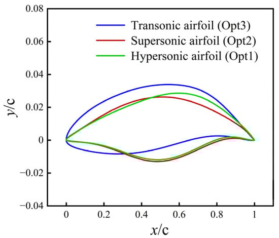
Figure 1.
Baseline geometries of the transonic, supersonic, and hypersonic airfoils adopted from the wide-Mach-number Pareto front optimization of Zhang et al. [23].
These designations reflect relative performance tendencies along the Pareto front rather than Mach-specific optimality. In the original optimization, the Pareto front was constructed only at Ma = 0.8 and Ma = 6. In the present study, the same three airfoils are reused without further optimization and are assigned to Ma = 0.8, 2, and 6, respectively, as anchor configurations for constructing continuous morphing trajectories. The Ma = 2 case represents an intermediate supersonic flow condition introduced solely for aerodynamic analysis, where the corresponding airfoil serves as a geometrically and aerodynamically transitional configuration between the transonic- and hypersonic-favored designs.
2.2. CST Parameterization and Geometric Reconstruction
To provide a unified analytic representation suitable for smooth morphing, all baseline airfoils are reconstructed using the Class–Shape Transformation method [32,33]:
where x ∈ [0, 1] is the normalized chordwise coordinate, and denotes the airfoil surface geometry. The term represents a small trailing edge thickness correction to ensure geometric consistency. Since all baseline airfoils considered in this study have a sharp trailing edge, is set to zero.
The class function
controls leading and trailing edge behavior, while the shape function
is expressed as an eighth-order Bernstein polynomial, and are the CST shape coefficients obtained by fitting the baseline airfoil geometry.
To illustrate the CST reconstruction quality, Figure 2 compares the original coordinate datasets and the CST-fitted curves for the three baseline airfoils. For the transonic, supersonic, and hypersonic airfoils, subplots Figure 2(a1,b1,c1) show the scattered original points together with the reconstructed surface, while Figure 2(a2,b2,c2) display the corresponding pointwise fitting errors. The CST representation matches all three geometries closely, the maximum fitting deviation is below 0.05% of the chord, ensuring that the CST representation retains the essential curvature characteristics of the reference shapes, including the “S-shaped” lower surfaces of supersonic and hypersonic airfoil.
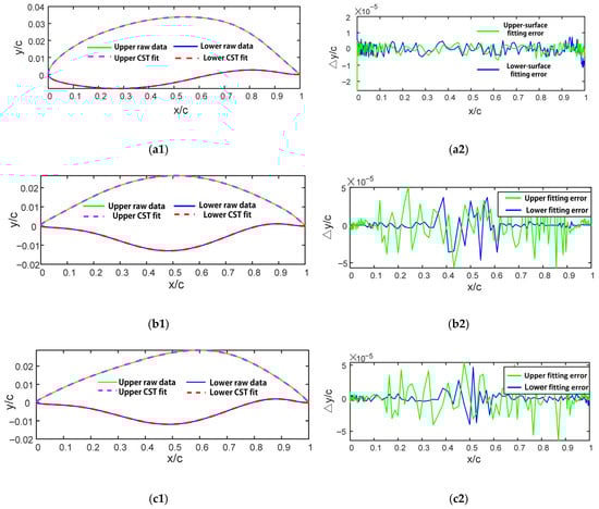
Figure 2.
CST parameterization validation: (a1,b1,c1) comparison between original coordinate points and CST-reconstructed curves for the transonic, supersonic, and hypersonic airfoils, respectively; (a2,b2,c2) corresponding pointwise fitting errors.
2.3. Morphing Trajectory and Mach Number Scheduling
To separate the effects of pure geometric morphing from those of morphing–acceleration coupling, as shown in Figure 3, two unsteady scenarios are designed in this study: Case 1 represents a pure geometric morphing process conducted at fixed Mach numbers, while Case 2 considers a coupled morphing–acceleration process in which the Mach number varies continuously during morphing. The flight altitudes shown in Figure 3 are included only to provide a conceptual reference for typical operating environments associated with different Mach number regimes. In the simulations, the corresponding freestream thermodynamic properties are prescribed accordingly, while altitude itself is not treated as an independent variable or optimized flight parameter.
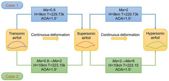
Figure 3.
Morphing workflow for both unsteady scenarios: Case 1 (pure geometric morphing at fixed Mach numbers) and Case 2 (morphing coupled with continuous Mach number variation).
The morphing airfoil geometry is generated by linearly interpolating the CST coefficient vectors according to the normalized morphing time :
where and denote the CST coefficients of the initial and target airfoil configurations, respectively. This interpolation strategy ensures continuous and smooth evolution of surface slope and curvature throughout the morphing process, avoiding non-physical oscillations or abrupt geometric changes.
In Case 1 (constant Mach morphing), the freestream Mach number remains fixed while the airfoil shape evolves continuously. At Ma = 0.8, the airfoil morphs from the transonic configuration to the supersonic configuration, whereas at Ma = 2 it morphs from the supersonic configuration to the hypersonic configuration. The morphing process is characterized by a total duration , and the aerodynamic flow fields are analyzed using the normalized time . Representative flow fields and aerodynamic coefficients are extracted at and 1 to characterize the evolution of the flow during different stages of the morphing process.
In Case 2 (coupled morphing–acceleration), the airfoil shape evolves in synchrony with a prescribed Mach number variation. Two successive Mach number transition ranges, Ma = 0.8–2 and Ma = 2–6, are considered to construct a representative morphing–acceleration scenario. Compared with Case 1, a more gradual acceleration process is adopted in Case 2 in order to ensure sufficient temporal resolution for resolving the unsteady evolution of shock structures under coupled morphing–acceleration conditions. Similarly to Case 1, all aerodynamic analyses are performed using the normalized time , and flow fields are sampled at the same normalized instants to enable consistent cross-regime comparison. The Mach number evolution is also described using the same normalized time framework. Mach number follows the same normalized time:
where and denote the initial and final Mach numbers of the corresponding stage.
This unified CST-based interpolation ensures that all morphing processes—whether at constant Mach number or accompanied by Mach number variation—maintain smooth curvature evolution suitable for analyzing the unsteady aerodynamic response across the transonic-to-hypersonic envelope.
2.4. Computational Domain and Grid Generation
A two-dimensional C–H-type structured grid is generated, extending 20c upstream, 100c downstream, and 75c toward the oblique far-field boundary, as shown in Figure 4. The inflow Mach number is fixed at Ma = 0.8 or 2 for the constant Mach cases, and follows the prescribed acceleration schedule in Case 2. The angle of attack is set to 1.5°. Far-field boundaries use characteristic-based conditions, while the airfoil surface is treated as an adiabatic no-slip wall. This setup ensures numerically stable and physically consistent simulations across all considered Mach regimes.
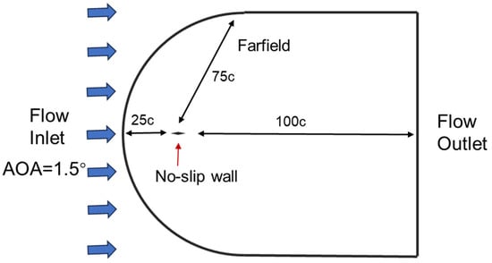
Figure 4.
Computational domain and boundary conditions.
As shown in Figure 5, the C–H-type structured grid is constructed based on a representative supersonic condition at Ma = 2 and employs local refinement around the leading edge, trailing edge, and anticipated shock regions to accurately resolve steep pressure gradients. Near-wall prism layers are generated with a first-layer height of approximately 4.2 × 10⁻⁶ m, resulting in wall values close to unity over the main aerodynamic surface. This near-wall resolution ensures adequate capture of viscous effects and shock–boundary-layer interaction (SBLI). The Ma = 2 condition is chosen as the reference case because it represents a typical supersonic regime in which both shock resolution and near-wall viscous accuracy are required. The same near-wall meshing strategy is applied across all Mach number regimes to maintain consistent viscous and shock-resolution characteristics.
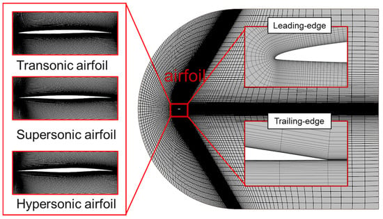
Figure 5.
C–H-type grid topology with leading edge and trailing edge refinement, and near-body mesh distributions for the transonic, supersonic, and hypersonic airfoils.
To verify grid independence, three mesh densities are examined using a steady supersonic baseline airfoil test case at Ma = 2 and , where shock structures and viscous effects are sufficiently strong to reveal sensitivity to grid resolution. The three meshes consist of a coarse grid (~5.6 × 10⁴ cells), a medium grid (~8.4 × 10⁴ cells), and a fine grid (~1.72 × 10⁵ cells). As summarized in Table 1, using the finest mesh (Mesh 3) as the reference, the lift-coefficient error decreases from 3.3% → 2.7% and the drag-coefficient error decreases from 3.2% → 2.9% when the grid is refined from Mesh 1 to Mesh 2. In order to balance accuracy and computational efficiency, Mesh 2 is selected for all subsequent simulations. Since the grid is designed and assessed under the Mach 2 condition, which represents the most demanding case in terms of combined shock resolution and near-wall accuracy, the same meshing strategy is adopted for all subsequent transonic and hypersonic simulations.

Table 1.
Lift coefficients
, drag coefficients
, and relative errors
of Mesh 1, Mesh 2, Mesh 3 (Ma = 2, α = 1.5°).
Figure 6 presents the distribution of wall along the airfoil surface for the representative supersonic case. Local differences between the upper and lower surfaces are observed in the immediate leading edge region, which may be associated with strong geometric curvature and local flow acceleration or stagnation effects.
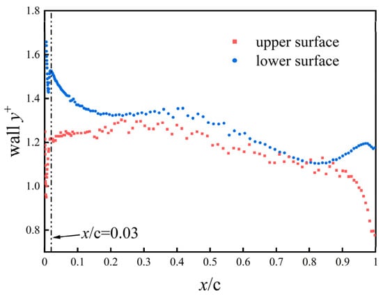
Figure 6.
Distribution of wall
along the supersonic airfoil surface (Ma = 2, α = 1.5°).
For the quantitative assessment of near-wall resolution, wall statistics are therefore evaluated over the main surface region , excluding the immediate leading edge. In this region, the reported values remain below 1.5 with mean values close to unity, as summarized in Table 2.
Table 2.
Statistical summary of wall
values on the supersonic airfoil surface (Ma = 2, α = 1.5°).
2.5. Dynamic Mesh and Unsteady Solver Settings
Mesh deformation is handled using the RBF dynamic mesh method [35] implemented in STAR- CCM+2022.R1 [36], which smoothly propagates boundary displacements through the interior mesh without cell distortion. The flow field is solved using the URANS equations [24] with the SST turbulence model [37] and second-order spatial and temporal discretization. As shown in Figure 7, the lift coefficient and drag coefficient histories obtained with Δt = 0.05 s, 0.1 s, and 0.2 s nearly overlap throughout the morphing process, indicating that the time integration is sufficiently converged. Considering both accuracy and computational efficiency, Δt = 0.1 s is adopted for the unsteady simulations.
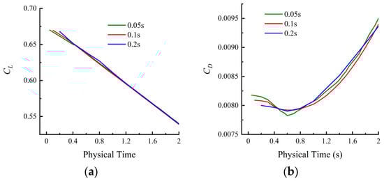
Figure 7.
Time-step independence assessment for ∆t = 0.2 s, 0.1 s, 0.05 s: (a) time histories of lift coefficient and (b) time histories of drag coefficient.
Within each physical time step, the inner iterations were continued until numerical convergence was achieved. Convergence was assessed using a combination of criteria: (i) the residuals of the continuity, momentum, energy, and turbulence equations were reduced by at least one order of magnitude, and (ii) the monitored aerodynamic coefficients (lift and drag) exhibited no noticeable temporal drift. The number of inner iterations per physical time step was therefore not fixed a priori, but determined adaptively to satisfy these convergence criteria.
All simulations were performed using Simcenter STAR-CCM+ (version 2022R1, double precision) on a local multi-core workstation (Windows 10, 64-bit) with 8 CPU cores. For the medium grid resolution (approximately 8.4 × 10⁴ cells), each unsteady simulation required approximately 5–7 h of wall-clock time, depending on the flow regime and morphing scenario.
2.6. Numerical Model Credibility and Methodological Consistency
Although no experimental dataset is available for the specific wide-Mach-number morphing trajectory considered in this study, the credibility of the present numerical model is supported through consistency with established numerical practices and physical principles. The simulations are performed using STAR-CCM+ with the k-ω SST turbulence model, which has been widely validated for shock–boundary-layer interaction and compressible viscous flows in transonic and supersonic regimes [37,38]. The turbulence modeling approach, near-wall treatment ( ≈ 1), and second-order spatial and temporal discretization adopted here are consistent with those employed in the referenced studies.
In addition, the RBF-based dynamic mesh technique ensures smooth mesh deformation during continuous airfoil morphing [34]. The predicted shock inclination and flow-turning behavior during coupled morphing–acceleration cases follow classical gas-dynamic relations, such as the θ-β-Ma number relationship [39], indicating that the governing compressible-flow mechanisms are reliably captured.
3. Results and Discussion
This section primarily focuses on the coupled morphing–acceleration scenario (Case 2), which represents a realistic high-speed flight process where airfoil geometry and freestream Mach number evolve simultaneously. The constant Mach morphing cases (Case 1) are first presented as reference configurations to isolate the pure geometric effect and to establish a physical baseline for interpreting the coupled results.
3.1. Case 1: Constant Mach Morphing as a Physical Reference
In this scenario, the freestream Mach number remains fixed while the airfoil geometry evolves according to the CST interpolation. Two Mach numbers—Ma = 0.8 (transonic) and Ma = 2 (supersonic)—are considered to isolate the pure geometric effect on compressible aerodynamic structures.
3.1.1. Transonic Morphing at Ma = 0.8
- •
- Pressure Contours
Figure 8 presents the pressure contours at four morphing instants (, , , and ) during the transition from the transonic airfoil to the supersonic airfoil at Ma = 0.8 and α = 1.5°. Although the freestream Mach number is subsonic, local acceleration over the upper surface produces a transonic pocket whose suction intensity increases progressively with time, the lower surface remains under positive pressure. The upper-surface flow evolves markedly: at a broad low-pressure region with a weak shock prevails, benefiting from the transonic airfoil’s blunter leading edge that delays shock formation; at , this is replaced by a distinct normal shock and a weak λ-shaped system near .
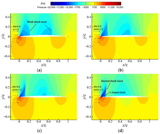
Figure 8.
Pressure contours during morphing at Ma = 0.8: (a)
, (b)
, (c)
, and (d)
.
- •
- Pressure coefficients
The evolution of the surface pressure coefficient () across the four morphing instants is shown in Figure 9 (suction plotted upward). As the airfoil deforms, three key changes emerge. The suction peak on the upper surface intensifies slightly and shifts forward, while the pressure distribution on the lower surface remains nearly invariant. Consequently, the area enclosed between the upper and lower curves contracts progressively with t/T increases, signaling a steady loss in net lift. The initial configuration () delivers the most favorable aerodynamic state, characterized by strong yet smooth suction and the weakest adverse pressure gradient.
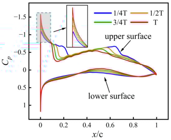
Figure 9.
Surface pressure-coefficient distribution at Ma = 0.8 for four morphing instants:
,
,
, and
.
- •
- Aerodynamic coefficients
Figure 10 quantitatively illustrates the evolution of aerodynamic characteristics during the airfoil morphing process at Mach 0.8. As the airfoil transitions from a transonic configuration to a supersonic configuration, the lift coefficient exhibits an approximately linear decreasing trend with the non-dimensional time t/T increases. Within the interval from and , the lift coefficient decreased by 19.4%. This lift loss is directly related to the gradual reduction in the area enclosed by the upper and lower surface pressure coefficient distributions (Figure 9). Concurrently, due to shock wave intensification, the drag coefficient increased by approximately 19%. The combined effect of these two factors resulted in a 28.8% reduction in the lift-to-drag ratio, indicating that the aerodynamic efficiency peaks during the initial phase of morphing, where the transonic configuration is most compatible with the transonic flow field. The high lift-to-drag ratio at the early morphing stage is mainly attributed to a low-drag interval, where decreases to approximately 0.0078 while remains moderate at about 0.63. This behavior is associated with the strong sensitivity of transonic shock structures to geometric variations, and is further facilitated by the relatively thin airfoil section (), which is favorable for reduced wave-drag penalties. These results highlight the high sensitivity of transonic flow fields to geometric parameter variations: under the fixed Mach 0.8 condition, even slight changes in airfoil geometry can trigger drastic alterations in the pressure field and aerodynamic coefficients.
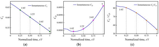
Figure 10.
Time histories of aerodynamic coefficients during morphing at Ma = 0.8: (a) lift coefficient
, (b) drag coefficient
, and (c) lift-to-drag ratio
.
3.1.2. Supersonic Morphing at Ma = 2
- •
- Pressure Contours
Figure 11 presents the pressure contours at four morphing instants (, , , and ) during the transition from the supersonic airfoil to the hypersonic airfoil at Ma = 0.8 and α = 1.5°. At all instants, oblique shock waves consistently appear near the airfoil’s leading and trailing edges, while a pronounced strong compression region forms in its leading edge area. Along the upper surface, a Prandtl-Meyer expansion [40] produces a smooth, monotonic decrease in pressure toward the trailing edge. The lower surface exhibits a structured yet gentle compression–expansion–compression pattern, consisting of a short leading edge compression zone (), a mid-chord expansion region (), and a mild recompression near the trailing edge (). The overall pressure distribution remains smooth and free of abrupt gradients throughout the morphing process.
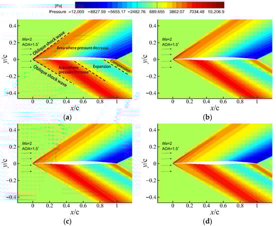
Figure 11.
Pressure contours during morphing at Ma = 2: (a)
, (b)
, (c)
, and (d)
.
- •
- Pressure coefficients
Figure 12 shows the evolution of the surface pressure coefficient under the constant Mach Ma = 2 condition. Both the upper and lower leading edges exhibit strong positive-pressure peaks, while the pressure on the upper surface decreases monotonically toward the trailing edge. The lower surface maintains a characteristic “double-S” distribution composed of an initial compression region, a mid-chord expansion region, and a recompression near the trailing edge. Unlike the Ma = 0.8 case, where the upper surface remains entirely under suction, the present supersonic condition displays a different pressure partition: from to 0.5, both surfaces lie within the positive-pressure range, and from to 1, the upper surface becomes a negative-pressure region while the lower surface remains at positive pressure, and their pressure difference generates lift.
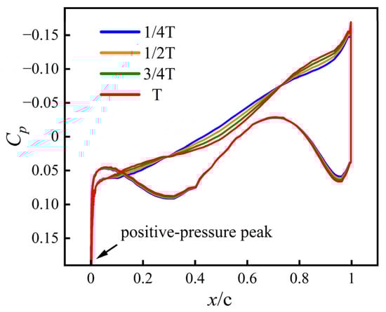
Figure 12.
Surface pressure-coefficient distribution at Ma = 2 for four morphing instants:
,
,
, and
.
The four curves are tightly clustered, indicating that the pressure-loading variation during morphing is very small—an expected outcome because both the initial and final geometries are designed for supersonic operation. Since negative values are plotted upward, the large leading edge positive-pressure spike extends beyond the visible axis range. Although the axis limits truncate part of this peak, its presence is clearly indicated by the steep initial rise near , consistent with the strong leading edge compression seen in the pressure contour plots.
- •
- Aerodynamic coefficients
Figure 13 quantitatively presents the changes in lift, drag, and lift-to-drag ratio during the airfoil’s morphing process from a supersonic configuration to a hypersonic configuration at Ma = 2. Within the morphing interval (from and ), the lift coefficient () exhibits a minor decreasing trend with a reduction of 1.4%, while the drag coefficient () shows a slight increase of 2.6%. Consequently, the lift-to-drag ratio decreases by 4.7%. This indicates that under the fixed Mach 2 condition, the overall aerodynamic characteristics of the airfoil remain stable during the morphing process.
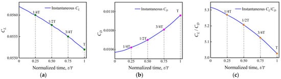
Figure 13.
Time histories of aerodynamic coefficients during morphing at Ma = 2: (a) lift coefficient
, (b) drag coefficient
, and (c) lift-to-drag ratio
.
Based on the pressure contours, pressure coefficient distributions, and aerodynamic coefficient plots presented, it is demonstrated that the supersonic flow field exhibits weak aerodynamic sensitivity, possessing an inherent robustness to smooth geometric deformation.
3.2. Case 2: Coupled Morphing–Acceleration as a Unified Transonic–Hypersonic Adaptation Process
This scenario represents the realistic flight of an accelerating high-speed vehicle, where both geometry and Mach number evolve simultaneously. The flow field undergoes a sequence of transonic, supersonic, and hypersonic transformations, coupled with curvature evolution.
3.2.1. Stage 1: Transonic ⟶ Supersonic (Ma = 0.8 ⟶ 2)
- •
- Pressure Contours
Figure 14 presents the pressure contour plots at four distinct moments during the morphing-acceleration coupled process (where the airfoil morphs from a transonic configuration to a supersonic configuration, with the Mach number increasing from 0.8 to 2 at an angle of attack of 1.5°). In the early stage of morphing (non-dimensional time ), with the Mach number approximately 1.1, a detached, quasi-bow shock wave structure is observed in the leading edge compression region. As the Mach number increases and the airfoil geometry evolves synchronously, this quasi-bow shock smoothly transitions into a well-defined oblique shock. The shock angle on the upper surface of the leading edge progressively decreases from the quasi-bow distribution state, sequentially reaching about 58°, 44°, and 35°. This trend aligns with the theoretical predication of the θ-β-Ma relation [38,39]. Due to the smaller local flow turning angle on the lower surface, its shock angle remains smaller than that on the upper surface throughout the entire evolution. Concurrently, with increasing t/T, the flow field pressure distribution gradually approaches the characteristic pattern of a typical Mach 2 flow: a compression–expansion structure forms on the upper surface, while the lower surface exhibits a compression–expansion–recompression flow pattern.
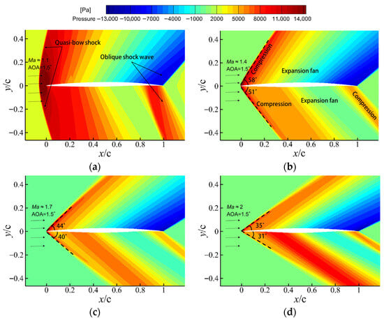
Figure 14.
Pressure contours during the coupled morphing–acceleration process from Ma = 0.8 to 2: (a)
, (b)
, (c)
, and (d)
.
- •
- Pressure coefficients
Figure 15 shows the surface pressure-coefficient evolution during the coupled morphing–acceleration process from Ma = 0.8 to 2. As the Mach number increases and the geometry transitions toward the supersonic configuration, the curves gradually converge, and the enclosed area between the upper and lower surfaces decreases, indicating a continuous reduction in lift. Both surfaces evolve toward smoother, more supersonic-like pressure distributions as increases, consistent with the pressure contour evolution shown in Figure 14.
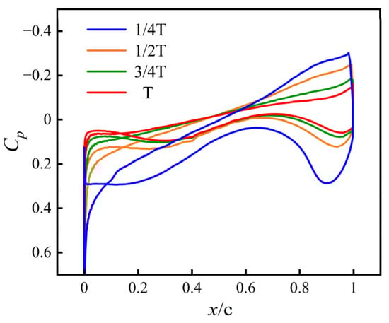
Figure 15.
Surface pressure-coefficient distribution during the coupled morphing–acceleration process from Ma = 0.8 to 2 for four morphing instants:
,
,
, and
.
- •
- Aerodynamic coefficients
Figure 16 illustrates the evolution of the surface aerodynamic coefficients during the coupled morphing process across the transition from Ma = 0.8 to Ma = 2. Between and , the lift coefficient decreases by 75%. The drag coefficient first increases and then decreases, with its maximum occurring near a freestream Mach number of approximately 1.2, where the flow experiences the influence of a detached, bow-like compression structure. Over the same interval, the lift-to-drag ratio decreases by 58.4%; most of this reduction occurs between and , which corresponds to the low supersonic phase; while the variation from to remains relatively small. This indicates that, in the supersonic stage, the coupling between Mach number acceleration and geometric morphing remains well coordinated.
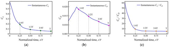
Figure 16.
Time histories of aerodynamic coefficients during the coupled morphing–acceleration process from Ma = 0.8 to 2: (a) lift coefficient
, (b) drag coefficient
, and (c) lift-to-drag ratio
.
- •
- Streamlines and vorticity at Ma = 1.1
Figure 17 presents the streamlines and vorticity visualization at Ma = 1.1, α = 1.5° with a grayscale pressure background. The background shading is shown only for reference, while the analysis focuses on the colored streamlines that indicate the local velocity magnitude. A distinct detached bow shock wave is observed upstream of the leading edge. The streamline above the surface deflects upward after passing through the shock wave, aligning its direction closely with the geometric contour of the upper surface. In contrast, the streamline below the surface deflects downward, with the flow approximating a nearly straight path. Further away from the airfoil, the streamlines gradually recover the freestream direction. Color variations along the streamlines indicate a local deceleration–acceleration pattern on the upper surface of the airfoil and a milder deceleration–acceleration–deceleration sequence on the lower surface.
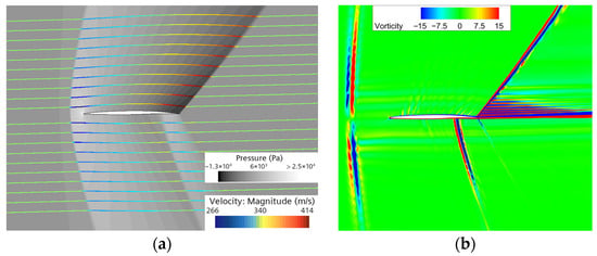
Figure 17.
Flow visualization at Ma = 1.1, α = 1.5°: (a) pressure contour and streamlines; (b) vorticity contour.
The vorticity contours reveal thin, elongated red–blue bands aligned with the locations of the bow-shaped compression region and the trailing edge shock. These bands form narrow, vertically oriented structures upstream and inclined layers near the upper and lower surfaces. In the wake, a sequence of horizontally distributed alternating red–blue patches appear.
3.2.2. Stage 2: Supersonic → Hypersonic (Ma = 2 → 6)
- •
- Pressure Contours
Figure 18 presents the pressure contour distributions at four normalized instants ( and 1) during the coupled morphing–acceleration process in which the Mach number increases from 2 to 6 and airfoil morphs from a supersonic configuration to a hypersonic configuration. Across all stages, the upper surface initially exhibits a leading edge compression region that progressively transitions into an expansion-dominated pressure field toward the mid- and aft-chord regions. On the lower surface, a consistent sequence of “compression → expansion → recompression’’ is maintained throughout the process. As the Mach number further increases, the shock angle decreases monotonically and the shock gradually moves closer to the airfoil surface. No shock oscillation or separation is observed at any stage, indicating that the morphing–acceleration trajectory remains aerodynamically stable.
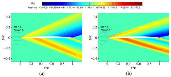
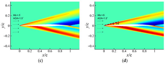
Figure 18.
Pressure contours during the coupled morphing–acceleration process from Ma = 2 to 6: (a)
, (b)
, (c)
, and (d)
.
- •
- Pressure coefficients
Figure 19 illustrates the evolution of the surface pressure coefficient () during the coupled morphing process across the transition from Ma = 2 to Ma = 6. The reduction in lift during acceleration is reflected in the evolution of the pressure-coefficient distributions. As Mach number rises, the curves on the two surfaces move toward each other: upper-surface suction weakens and lower-surface compression diminishes. The lower surface’s “double-S” pattern, while still identifiable, becomes progressively smoother. The net effect is a systematic decrease in the enclosed area between the curves, which correlates directly with the declining lift force.
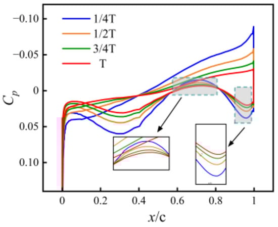
Figure 19.
Surface pressure-coefficient distribution during the coupled morphing–acceleration process from Ma = 2 to 6 for four morphing instants:
,
,
, and
.
- •
- Aerodynamic Coefficients
Figure 20 presents the variation patterns of aerodynamic coefficients during the coupled morphing process across the transition from Ma = 2 to Ma = 6. Within the interval from the non-dimensional time and , the lift coefficient sharply decreases by 60%, which is consistent with the observed reduction in the area enclosed by the pressure coefficient distribution in Figure 19. Simultaneously, the drag coefficient declines by 50%, aligning with the observed decrease in the leading edge shock angle and weakening of shock intensity shown in Figure 18. The combined effect of these factors results in a 15.8% reduction in the lift-to-drag ratio, indicating a moderate decline in the aerodynamic efficiency of the airfoil as the flow field transitions into a compression-dominated state

Figure 20.
Time histories of aerodynamic coefficients during the coupled morphing–acceleration process from Ma = 2 to 6: (a) lift coefficient
, (b) drag coefficient
, and (c) lift-to-drag ratio
.
- •
- Streamline and Vorticity Structures at Ma = 2 and Ma = 6
Figure 21 and Figure 22 illustrate the streamline-pressure fields and vorticity fields at Mach 2 and Mach 6, respectively. The focus of this section’s analysis lies on the streamline plots. To more clearly display streamline velocities, a grayscale pressure contour serves as the background, while the streamlines are rendered in color.
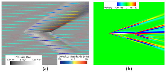
Figure 21.
Flow visualization at Ma = 2, α = 1.5°: (a) pressure contour and streamlines; (b) vorticity contour.
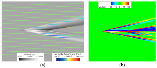
Figure 22.
Flow visualization at Ma = 6, α = 1.5°: (a) pressure contour and streamlines; (b) vorticity contours.
At Mach 2, the streamlines decelerate sharply under the influence of the leading edge oblique shock, accelerate as they pass through the Prandtl-Meyer expansion fan, and then decelerate again at the trailing edge shock, forming a coherent “compression–expansion–recompression” cycle. This characteristic is also reflected in the vorticity field (Figure 21b): the strong shear layers perfectly coincide with the shock locations. Well-defined boundary layer vorticity layers with opposite signs form on the upper and lower surfaces of the airfoil, which merge downstream in the wake region into a stable horizontal vorticity band.
As shown in Figure 22b, when the Mach number is 6, the flow field transitions to a multi-scale, disordered state. Driven by larger velocity gradients resulting from stronger shocks, the magnitude of vorticity nearly doubles compared to Mach 2 (±15), reaching approximately ±30. Here, the interaction between shocks and shear layers, along with potential shock-shock interference as the reduced shock angles bring high-Mach flow closer to the airfoil surface, becomes the dominant factor. The previously orderly wake vorticity band breaks down into discrete vorticity clusters.
A comprehensive comparison reveals that as the Mach number increases, the vorticity field evolves from an ordered, shear-dominated pattern at low supersonic speeds to a mode dominated by intense multi-scale interactions at hypersonic speeds. This transition reflects a significant increase in the complexity of the flow field’s energy compression, vorticity generation, and downstream transport processes with increasing Mach number.
The coupled morphing–acceleration process demonstrates that continuous geometric deformation can effectively guide the flow across speed regimes without triggering abrupt shock motion or separation. Unlike the constant Mach cases, this coupled adaptation reveals a synergistic mechanism wherein smooth curvature modulation and Mach number evolution jointly regulate shock system migration and wake vorticity development.
4. Conclusions
This study investigates the unsteady aerodynamic response of a morphing airfoil across a wide Mach number envelope (Ma = 0.8–6) using CST-based continuous geometric interpolation. Three representative airfoils optimized for transonic, supersonic, and hypersonic conditions serve as the anchor shapes, and both constant Mach and coupled morphing–acceleration scenarios are examined. The conclusions below emphasize the underlying aerodynamic mechanisms governing the variation in lift, drag, shock structures, and wake dynamics during continuous morphing.
- Continuous curvature variation ensures a smooth and stable deformation process. The CST interpolation eliminates slope discontinuities, enabling shock structures to migrate steadily along the surface with no oscillation, separation, or abrupt load changes throughout all simulations.
- The transonic regime exhibits the strongest sensitivity to shape evolution. At Ma = 0.8, the upper-surface suction peak shifts noticeably during the morphing process, resulting in a 19.4% decrease in lift and a 19% increase in drag, which together cause a 28.8% reduction in lift-to-drag ratio. This behavior highlights the pronounced coupling between shock position and pressure distribution in transonic flows.
- The supersonic deformation stage remains highly robust. At Ma = 2, the characteristic “compression–expansion–recompression’’ structure is preserved, and the aerodynamic response is mild, with lift changing by only 1.4% and drag by 2.6% across the morphing interval, demonstrating the inherent robustness of supersonic flow fields to smooth geometric deformation.
- Across the entire wide-speed-range envelope (Ma = 0.8–6), the morphing airfoil maintains L/D > 4, indicating a consistently acceptable aerodynamic efficiency for conceptual high-speed lifting surface design compared with fixed-geometry configurations operating far from their design points.
- The results indicate a common tendency in flow adaptation across transonic, supersonic, and hypersonic regimes. Continuous geometric deformation influences the organization of compression and expansion wave systems and is accompanied by systematic shock migration. Meanwhile, the wake vorticity field exhibits a gradual transition from organized shear layers to more complex vortical structures as the Mach number increases, reflecting differing sensitivities of the flow field to geometric perturbations.
In summary, the present results demonstrate that continuous airfoil morphing provides a smooth and effective aerodynamic adaptation pathway over a wide Mach number range, avoiding abrupt flow-state transitions commonly encountered in fixed-geometry configurations. The aerodynamic insights obtained in this study establish a physical basis at the conceptual level for the design of adaptive high-speed lifting surfaces.
Although the present work focuses on two-dimensional unsteady aerodynamic mechanisms, the findings offer useful guidance for future engineering-oriented studies. Future research should extend the proposed framework to three-dimensional morphing wings, where spanwise flow effects, structural deformation modes, and aeroelastic interactions may play important roles. In addition, the integration of morphing kinematics with control strategies and adaptive materials will be essential for advancing toward practical high-speed morphing configurations. Related three-dimensional morphing wing concepts, including those based on variable-thickness lattice or cellular architectures, will be explored in dedicated future investigations.
Author Contributions
Conceptualization, L.Z. and R.Z.; methodology, L.Z.; software, L.Z.; validation, L.Z. and R.Z.; formal analysis, L.Z.; investigation, L.Z., X.S.; resources, Z.W.; data curation, L.Z.; writing—original draft preparation, L.Z.; writing—review and editing, L.Z. and R.Z.; visualization, L.Z.; supervision, Z.W.; project administration, Y.Y. and Z.W.; funding acquisition, Y.Y. and Z.W. All authors have read and agreed to the published version of the manuscript.
Funding
This work is supported by National Natural Science Foundation of China (Grant No. U2541234).
Data Availability Statement
The data presented in this study are available from the corresponding author upon reasonable request.
Acknowledgments
The authors thank all colleagues and collaborators for their insightful discussions.
Conflicts of Interest
The authors declare no conflicts of interest.
Abbreviations
The following abbreviations are used in this manuscript:
| CST | Class–Shape Transformation |
| URANS | Unsteady Reynolds-Averaged Navier–Stokes |
| RBF | Radial Basis Function |
| CFD | Computational Fluid Dynamics |
| SST | Shear Stress Transport |
| SBLI | Shock–Boundary-Layer Interaction |
| NSGA-II | Nondominated Sorting Genetic Algorithm II |
| AOA | Angle of Attack |
References
- Barbarino, S.; Bilgen, O.; Ajaj, R.M.; Friswell, M.I.; Inman, D.J. A review of morphing aircraft. J. Intell. Mater. Syst. Struct. 2011, 22, 823–877. [Google Scholar] [CrossRef]
- Chu, L.; Li, Q.; Gu, F.; Du, X.; He, Y.; Deng, Y. Design, modeling, and control of morphing aircraft: A review. Chin. J. Aeronaut. 2022, 35, 220–246. [Google Scholar] [CrossRef]
- Chen, S.; Jia, M.; Liu, Y.; Gao, Z. Deformation modes and key technologies of aerodynamic layout design for morphing aircraft. Acta Aeronaut. Astronaut. Sin. 2024, 45, 6. [Google Scholar]
- Kabir, A.; Al-Obaidi, A.S.M. A survey of trailing-edge morphing airfoil studies: Configurations, performance, and applications. In Proceedings of the 9th International Conference on Recent Advances and Innovations in Engineering (ICRAIE), Kuala Lumpur, Malaysia, 23–24 August 2025; IEEE: New York, NY, USA, 2025; pp. 183–188. [Google Scholar]
- Weisshaar, T.A. Morphing aircraft technology—New shapes for aircraft design. In Multifunctional Structures/Integration of Sensors and Antennas; RTO: Paris, France, 2006. [Google Scholar]
- Manor, D.; Johnson, D. Landing the wave-rider: Challenges and solutions. In Proceedings of the AIAA/CIRA 13th International Space Planes and Hypersonic Systems and Technologies Conference, Capua, Italy, 16–20 May 2005; Paper No. 3201; AIAA: Reston, VI, USA, 2005. [Google Scholar]
- National Research Council. Decadal Survey of Civil Aeronautics: Foundation for the Future; National Academies Press: Washington, DC, USA, 2006. [Google Scholar]
- Leite, B.; Afonso, F.; Suleman, A. Aerodynamic shape optimization of a symmetric airfoil from subsonic to hypersonic flight regimes. Fluids 2022, 7, 353. [Google Scholar] [CrossRef]
- Xie, Z.; Zhao, Z.T.; Huang, W.; Liu, C.Y.; Choubey, G. Aerodynamic analysis of hypersonic gliding vehicles with wide-speed range based on the cuspidal waverider. Fluid Dyn. 2024, 59, 622–637. [Google Scholar] [CrossRef]
- Tauber, M.E.; Menees, G.P.; Adelman, H.G. Aerothermodynamics of transatmospheric vehicles. J. Aircr. 1987, 24, 594–602. [Google Scholar] [CrossRef]
- Viviani, A.; Pezzella, G. Next generation launchers aerodynamics. TC 2012, 37, 661. [Google Scholar]
- Burdette, D.A.; Martins, J.R.R.A. Design of a transonic wing with an adaptive morphing trailing edge via aerostructural optimization. Aerosp. Sci. Technol. 2018, 81, 192–203. [Google Scholar] [CrossRef]
- Schuet, S.; Lombaerts, T.; Acosta, D.; Wheeler, K.; Kaneshige, J. An adaptive nonlinear aircraft maneuvering envelope estimation approach for online applications. In Proceedings of the AIAA Guidance, Navigation, and Control Conference, National Harbor, MD, USA, 9–13 January 2014; Paper No. 0268; AIAA: Reston, VI, USA, 2014. [Google Scholar]
- Mowla, M.N.; Asadi, D.; Durhasan, T.; Jafari, J.R.; Amoozgar, M. Recent advancements in morphing applications: Architecture, artificial intelligence integration, challenges, and future trends—A comprehensive survey. Aerosp. Sci. Technol. 2025, 161, 110102. [Google Scholar] [CrossRef]
- Mangano, M.; Martins, J.R.R.A. Multipoint aerodynamic shape optimization for subsonic and supersonic regimes. J. Aircr. 2021, 58, 650–662. [Google Scholar] [CrossRef]
- Johnson, D.; Thomas, R.; Manor, D. Stability and control analysis of a wave-rider TSTO second stage. In Proceedings of the 10th AIAA/NAL-NASDA-ISAS International Space Planes and Hypersonic Systems and Technologies Conference, Kyoto, Japan, 24–27 April 2001; Paper No. 2001-1834; AIAA: Reston, VI, USA, 2001. [Google Scholar]
- Zhang, Y.; Luo, J.; Zheng, Y.; Liu, Y. Aerodynamic Optimization of Airfoil in Wide Range of Operating Conditions Based on Reinforcement Learning. Aerospace 2025, 12, 443. [Google Scholar] [CrossRef]
- Yu, J.; Zhou, G.; Han, Q.; Jia, H.; Zhang, P.; Liu, S.; Li, W. Data mining of Pareto-optimal wide-Mach-number-range airfoil shapes. In Proceedings of the 2nd Aerospace Frontiers Conference (AFC 2025), Beijing, China, 11–14 April 2025; Springer Nature: Singapore, 2025; pp. 118–128. [Google Scholar]
- Wei, C.; Li, R.; Xu, P.; Duan, Y.; Wang, S.; Chang, Y. Aerodynamic shape optimization for a hypersonic vehicle flying over a range of speeds. J. Phys. Conf. Ser. 2025, 3006, 012043. [Google Scholar] [CrossRef]
- Longtin Martel, S.; Bashir, M.; Botez, R.M.; Wong, T. A Pareto multi-objective optimization of a camber morphing airfoil using non-dominated sorting genetic algorithm. In Proceedings of the AIAA SciTech 2023 Forum, San Diego, CA, USA, 23–27 January 2023; Paper No. 1583; AIAA: Reston, VI, USA, 2023. [Google Scholar]
- Liu, B.; Liang, H.; Han, Z.H.; Yang, G. Surrogate-based aerodynamic shape optimization of a morphing wing considering a wide Mach-number range. Aerosp. Sci. Technol. 2022, 124, 107557. [Google Scholar] [CrossRef]
- Mangano, M. Multi-Point Aerodynamic Shape Optimization for Airfoils and Wings at Supersonic and Subsonic Regimes. Master’s Thesis, Delft University of Technology, Delft, The Netherlands, 20 May 2019. [Google Scholar]
- Zhang, Y.; Han, Z.; Zhou, Z.; Tang, J.; Zhang, K.; Song, W. Aerodynamic design optimization of wide-Mach-number-range airfoils for hypersonic vehicles. Acta Aerodyn. Sin. 2021, 39, 111–127. [Google Scholar]
- Szulc, O.; Doerffer, P.; Flaszyński, P.; Suresh, T. Numerical modelling of shock wave–boundary layer interaction control by passive wall ventilation. Comput. Fluids 2020, 200, 104435. [Google Scholar] [CrossRef]
- Anderson, J.D. Modern Compressible Flow: With Historical Perspective; McGraw-Hill: New York, NY, USA, 2003. [Google Scholar]
- Gaitonde, D.V. Progress in shock wave/boundary layer interactions. Prog. Aerosp. Sci. 2015, 72, 80–99. [Google Scholar] [CrossRef]
- John, B.; Kulkarni, V.N.; Natarajan, G. Shock wave–boundary layer interactions in hypersonic flows. Int. J. Heat Mass Transf. 2014, 70, 81–90. [Google Scholar] [CrossRef]
- Chen, Y. Shock wave–boundary layer interaction: A survey of recent development. Highlights Sci. Eng. Technol. 2024, 1, A43. [Google Scholar] [CrossRef]
- Zheng, C.; Feng, Y.; Zheng, X. Effect of bulk viscosity on the hypersonic compressible turbulent boundary layer. J. Fluid Mech. 2024, 982, A24. [Google Scholar] [CrossRef]
- Viola, N.; Roncioni, P.; Gori, O.; Fusaro, R. Aerodynamic Characterization of Hypersonic Transportation Systems and Its Impact on Mission Analysis. Energies 2021, 14, 3580. [Google Scholar] [CrossRef]
- Pezzella, G.; Viviani, A. Aerodynamic analysis of a high-speed aircraft from hypersonic down to subsonic speeds. Mater. Res. Proc. 2023, 3, 230–233. [Google Scholar]
- Kulfan, B.M. Universal parametric geometry representation method. J. Aircr. 2008, 45, 142–158. [Google Scholar] [CrossRef]
- Kulfan, B.; Bussoletti, J. Fundamental parametric geometry representations for aircraft component shapes. In Proceedings of the 11th AIAA/ISSMO Multidisciplinary Analysis and Optimization Conference, Portsmouth, VA, USA, 6–8 September 2006; AIAA: Reston, VI, USA, 2006. [Google Scholar]
- Xiang, J.; Liu, K.; Li, D.; Cheng, C.; Sha, E. Unsteady aerodynamic characteristics of a morphing wing. Aircr. Eng. Aerosp. Technol. 2019, 91, 1–9. [Google Scholar] [CrossRef]
- Zhang, Y.; Li, T.; Liu, Z.; Yu, M.; Shao, J.; Price, W.G.; Hudson, D. RBF-based interpolation and its application in flow–structure interaction. In Proceedings of the ISOPE International Ocean and Polar Engineering Conference, Shanghai, China, 11–16 October 2020; ISOPE: Cupertino, CA, USA, 2020. [Google Scholar]
- Blazek, J. Computational Fluid Dynamics: Principles and Applications; Butterworth-Heinemann: Oxford, UK, 2015. [Google Scholar]
- Menter, F.R. Two-equation eddy-viscosity turbulence models for engineering applications. AIAA J. 1994, 32, 1598–1605. [Google Scholar] [CrossRef]
- Deshpande, A. Unsteady Dynamics of Shock-Wave Boundary-Layer Interactions. Ph.D. Thesis, Purdue University, West Lafayette, IN, USA, 2021. [Google Scholar]
- Mehta, R.C. Exact solutions to the oblique shock wave equation. In Proceedings of the World Congress on Aeronautics, Nano, Bio, Robotics, and Energy, Incheon, Republic of Korea, 25–28 August 2015. [Google Scholar]
- Silnikov, M.V.; Chernyshov, M.V.; Uskov, V.N. Analytical solutions for Prandtl–Meyer wave—Oblique shock overtaking interaction. Acta Astronaut. 2014, 99, 175–183. [Google Scholar] [CrossRef]
Disclaimer/Publisher’s Note: The statements, opinions and data contained in all publications are solely those of the individual author(s) and contributor(s) and not of MDPI and/or the editor(s). MDPI and/or the editor(s) disclaim responsibility for any injury to people or property resulting from any ideas, methods, instructions or products referred to in the content. |
© 2026 by the authors. Licensee MDPI, Basel, Switzerland. This article is an open access article distributed under the terms and conditions of the Creative Commons Attribution (CC BY) license.