Robust MPS-INS UKF Integration and SIR-Based Hyperparameter Estimation in a 3D Flight Environment

Abstract

This study introduces a pose estimation algorithm integrating an Inertial Navigation System (INS) with an Alternating Current (AC) magnetic field-based navigation system, referred to as the Magnetic Positioning System (MPS), evaluated using a 6 Degrees of Freedom (DoF) drone. The study addresses significant challenges such as the magnetic vector distortions and model uncertainties caused by motor noise, which degrade attitude estimation and limit the effectiveness of traditional Extended Kalman Filter (EKF)-based fusion methods. To mitigate these issues, a Tightly Coupled Unscented Kalman Filter (TC UKF) was developed to enhance robustness and navigation accuracy in dynamic environments. The proposed Unscented Kalman Filter (UKF) demonstrated a superior attitude estimation performance within a 6 m coil spacing area, outperforming both the MPS 3D LS (Least Squares) and EKF-based approaches. Furthermore, hyperparameters such as alpha, beta, and kappa were optimized using the Sequential Importance Resampling (SIR) process of the Particle Filter. This adaptive hyperparameter adjustment achieved improved navigation results compared to the default UKF settings, particularly in environments with high model uncertainty.

1. Introduction

To mitigate the integration errors of the INS, a GNSS (Global Navigation Satellite System) is often employed. However, GNSS performance degrades when the Line of Sight (LOS) between the receiver and satellites is obstructed, or when signal attenuation occurs due to surrounding environmental factors. In contrast, artificial magnetic fields enable navigation without requiring LOS, and are less affected by signal attenuation in environments where GNSS signals are weak, such as underwater or underground regions.

Due to these advantages, both Direct Current (DC)-based and Alternating Current (AC)-based magnetic navigation methods have been proposed [1,2,3,4]. Studies have shown that AC magnetic navigation provides a larger navigation area at the same power level compared to DC magnetic navigation and exhibits superior accuracy. By leveraging these benefits of AC magnetic fields, our research group has developed a navigation system called the Magnetic Positioning System (MPS) based on AC magnetic fields [3,5].

For AC magnetic field-based navigation, coil models such as the dipole model and the circular coil model have been proposed. The dipole model exhibits uncertainties near the source point, but remains efficient within a suitable range and is mathematically simple, offering high computational efficiency. However, when expanding the range for navigation, the efficiency of the dipole model declines. This is particularly evident near the source coil, where the dipole model significantly deviates from the actual measurements, leading to a sharp degradation in performance. To address these limitations, the circular coil model was proposed, demonstrating reduced uncertainties near the coil while maintaining a computational efficiency nearly equivalent to that of the dipole model [6,7].

Research on magnetic–inertial navigation using the MPS has also been conducted in indoor environments. The experimental results revealed that in indoor settings, eddy currents caused by reinforced concrete structures lead to distortions in the Z-axis during pure magnetic field navigation. To mitigate these distortions, a study was conducted to integrate 2D (dimension) magnetic field navigation with a 1D range sensor, effectively reducing Z-axis errors for improved navigation performance [8].

Outdoor experiments on magnetic–inertial navigation were also conducted. Unlike in indoor environments, it was observed that the influence of eddy currents was significantly reduced in outdoor settings. As a result, accurate navigation was achieved using pure magnetic field navigation within a $6 \mathrm{m}\times 6 \mathrm{m}$ diagonal coil spacing area. Furthermore, navigation experiments were extended to a larger area of $16 \mathrm{m}\times 16 \mathrm{m}$, surpassing the indoor experiments conducted in the $6 \mathrm{m}\times 6 \mathrm{m}$ range. However, in the most expanded range, the performance of magnetic-based navigation was found to degrade due to signal occlusion of the magnetic vectors. To address this issue, Tightly Coupled structure sensor fusion was proposed [9,10].

Previous research on the MPS was limited to 2D magnetic field navigation or evaluations using a UGV (Unmanned Ground Vehicle) restricted to 3DoF (Degrees of Freedom) motion in outdoor environments. In contrast, this study utilized a drone capable of 6DoF motion to evaluate the performance of magnetic navigation in a $6 \mathrm{m}\times 6 \mathrm{m}$ area. The experimental results revealed that the 6DoF motion and motor noise of the drone caused a significant increase in model uncertainty near the coil. Consequently, magnetic vector signals were distorted in this region, leading to a decline in the attitude estimation performance of magnetic-based navigation. Similarly, navigation performance using an EKF (Extended Kalman Filter)-based approach, which was considered in previous methods, also deteriorated. EKF achieves optimal results when noise follows a Gaussian distribution. However, in environments where model uncertainty increases due to motor noise and 6DoF motion, such as in this experiment, the performance of EKF cannot be guaranteed. Therefore, the UKF (Unscented Kalman Filter) was considered a more suitable filter for environments like the one in this study [11,12,13,14].

Unlike the EKF, the UKF does not require linearization, making it more robust to nonlinearity. Additionally, the UKF has demonstrated greater resilience to model uncertainties compared to the EKF. However, in traditional UKF implementations, as the state dimension increases, the estimation region of sigma points expands, leading to performance degradation. To address this issue, the Scaled Unscented Transformation was proposed to regulate the sigma point estimation region [15]. By tuning the hyperparameters alpha, beta, and kappa, sigma points can be rearranged to conform to specific distributions, including non-Gaussian distributions. Studies have been conducted on the influence of these hyperparameters on UKF performance, along with methods for determining the appropriate settings [16,17,18,19].

Previous research [16,17,18,19] has shown that using likelihood as the objective function is effective. Through parameter adjustment, the log-likelihood value was optimized, enabling the estimation of the hyperparameters. In this study, the Sequential Importance Resampling (SIR) process, commonly used in Particle Filters, was employed to estimate the hyperparameters through resampling based on weight. The UKF navigation results using the converged hyperparameters derived through this process outperformed those obtained with UKF configurations using commonly preset hyperparameter values.

The contributions of this study are as follows. First, the navigation performance of the Magnetic Positioning System (MPS) was evaluated in a 6DoF environment using a drone. Second, through the design of a Tightly Coupled UKF (TC UKF), the navigation performance during drone flight demonstrated superior attitude estimation compared to traditional EKF-based methods. Third, the UKF using hyperparameters estimated through the SIR process of the Particle Filter outperformed the UKF with commonly preset hyperparameter values.

The remainder of this paper is organized as follows: Section 2 introduces the sensor integration framework for MPS/INS, describing the measurement model and the TC UKF integration approach, along with the estimation of the UKF hyperparameters using the SIR process. Section 3 presents an analysis of the magnetic vector errors occurring during flight, including details of the experimental environment and the characteristics of datasets with different types of model uncertainty. Section 4 discusses the navigation results, comparing the performance of a conventional UKF and SUKF (SIR-UKF) under various experimental conditions, Finally, Section 5 concludes the paper, summarizing key findings and suggesting potential directions for future research.

2. Sensor Integration MPS/INS

2.1. Measurement Description and UKF Tightly Coupled Integration

This section introduces the measurement model and the Tightly Coupled integration approach of the UKF. Figure 1 illustrates the MPS process.

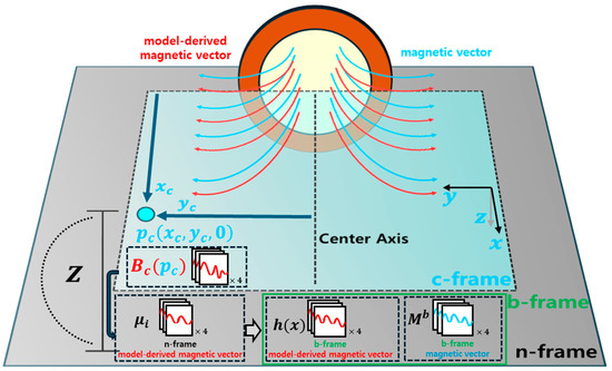
Figure 1. MPS magnetic field vector.

To model the AC magnetic field at each coil (500, 600, 700, and 800 Hz), the magnetic field is first expressed in the c-frame (coil frame), which is defined relatively to the plane centered at the coil. In the c-frame, the axis parallel to the coil’s center axis is defined as the x-axis, the axis perpendicular to the center axis is defined as the y-axis, and the downward direction is defined as the z-axis. The magnetic field vector ${\mathit{B}}_c$ at a specific point ${\mathit{p}}_c(x_c,y_c,0)$ in the c-frame is derived from the model. The n-frame (navigation frame) serves as the local reference frame for navigation, with its origin set at the center of the 6 $\times$ 6 m navigation area. Additionally, the c-frame and n-frame differ by the height Z, which corresponds to the center height of the coil. All navigation results are expressed in the n-frame. Therefore, to convert the model-derived magnetic field vector from the c-frame to the n-frame, a Direction Cosine Matrix (DCM) is applied.

The actual magnetic field vector is measured in the b-frame (body frame), which is defined relative to the drone. Therefore, to implement the Tightly Coupled integration in this study, the model-derived magnetic field vector must be aligned with the measured magnetic field vector. To achieve this, the model-derived magnetic field vector in the n-frame is converted to the b-frame using a DCM. The detailed mathematical derivation of this transformation is presented in Equations (1)–(8).

Based on previous studies [6,9], the magnetic vector ${\mathit{\mu }}_i$ in the $n$-frame with the application of the circular coil model can be expressed as shown in Equations (1)–(3).

$${\mathit{\mu }}_i={\mathit{C}}_c^n·{\mathit{B}}_c\left({\mathit{p}}_c\right)$$

(1)

$${\mathit{B}}_c\left({\mathit{p}}_c\right)=\begin{array}{c}\left[\begin{array}{l}{\displaystyle \frac{\gamma }{\sqrt{x_c^2+{\left(y_c+a\right)}^2}}}·\left({\displaystyle \frac{a^2-x_c^2-y_c^2}{x_c^2+{\left(y_c-a\right)}^2}}·{\displaystyle \frac{\pi }{2}}\left[1-{\displaystyle \sum _{i=1}^{\infty }}{\left({\displaystyle \frac{\left(2i-1\right)‼}{\left(2i\right)!}}·t^i\right)}^2·{\displaystyle \frac{1}{2i-1}}\right]+{\displaystyle \frac{\pi }{2}}\left[1+{\displaystyle \sum _{i=1}^{\infty }}{\left({\displaystyle \frac{\left(2i-1\right)‼}{\left(2i\right)!}}·t^i\right)}^2\right]\right)\\ {\displaystyle \frac{\gamma ·x_c}{y_c·\sqrt{x_c^2+{\left(y_c+a\right)}^2}}}·\left({\displaystyle \frac{a^2+x_c^2+y_c^2}{x_c^2+{\left(y_c-a\right)}^2}}·{\displaystyle \frac{\pi }{2}}\left[1-{\displaystyle \sum _{i=1}^{\infty }}{\left({\displaystyle \frac{\left(2i-1\right)‼}{\left(2i\right)!}}·t^i\right)}^2·{\displaystyle \frac{1}{2i-1}}\right]-{\displaystyle \frac{\pi }{2}}\left[1+{\displaystyle \sum _{i=1}^{\infty }}{\left({\displaystyle \frac{\left(2i-1\right)‼}{\left(2i\right)!}}·t^i\right)}^2\right]\right)\\ 0\end{array}\right]\end{array}$$

(2)

$$\gamma ={\displaystyle \frac{{\mu }_0·I}{2\pi }} ,\hspace{1em}\hspace{1em}{\mu }_0=4\pi \times {10}^{-7}{\displaystyle \frac{\mathrm{H}}{m}},\hspace{1em}\hspace{1em}{t}^2={\displaystyle \frac{4a·y_c}{x_c^2+{\left(y_c+a\right)}^2}}$$

(3)

Here, ${\mathit{C}}_c^n$ represents the DCM that transforms from the coil frame to the $n$-frame, and ${\mathit{B}}_c\left({\mathit{p}}_c\right)$ denotes the magnetic vector ${\mathit{B}}_c$ at position ${\mathit{p}}_c$ in the coil coordinate system. The measurement model is presented in Equation (4).

$$h\left(\mathit{x}\right)={\left[\begin{array}{c}{\mathit{C}}_n^b·{\mathit{\mu }}_{500hz}\\ {\mathit{C}}_n^b·{\mathit{\mu }}_{600hz}\\ {\mathit{C}}_n^b·{\mathit{\mu }}_{700hz}\\ {\mathit{C}}_n^b·{\mathit{\mu }}_{800hz}\end{array}\right]}_{12\times 1}$$

(4)

In Equation (4), the magnetometer measurement is composed of four components, which represent three-dimensional vectors from four simultaneous AC magnetic fields. In practice, one concurrent magnetic field vector is acquired and digitally processed in the DSP module for synchronized demodulation, separating each frequency component. A detailed explanation can be found in [5].

Also, note that the magnetic vector generated in the 500–800 Hz range is multiplied by ${\mathit{C}}_n^b$ to transform it into a value measured in the body frame. This process involves computing the observation matrix $\mathit{H}$ by differentiating the observation model $h\left(\mathit{x}\right)$ given in (5) with respect to changes in position $\mathit{p}$ and attitude $\mathit{\varphi }$, respectively.

$$\mathit{H}={\displaystyle \frac{\partial h\left(\mathit{x}\right)}{\partial \mathit{x}}}={\left[{\displaystyle \frac{\partial h\left(\mathit{x}\right)}{\partial \mathit{p}}}{\displaystyle \frac{\partial h\left(\mathit{x}\right)}{\partial \mathit{\varphi }}}\right]}_{6\times 1}$$

(5)

The observation matrix is utilized to apply the Least Squares (LS) method, as shown in Equation (6), to obtain measurements for MPS magnetic field navigation, obtaining the error estimate of position $\delta \mathit{p}$ and attitude perturbation $\delta \mathit{\varphi }$, respectively. By employing Equations (7) and (8), the position $\mathit{p}$ and attitude $\mathit{q}$, expressed in quaternion form, are obtained from the MPS.

$${\left[\begin{array}{c}\delta \mathit{p}\\ \delta \mathit{\varphi }\end{array}\right]}_{6\times 1}={\left({\mathit{H}}^{\mathrm{T}}·\mathit{H}\right)}^{-1}·{\mathit{H}}^{\mathrm{T}}·\left({\left[\begin{array}{c}{\mathit{M}}_{500\mathrm{h}\mathrm{z}}^{\mathrm{b}}\\ {\mathit{M}}_{600\mathrm{h}\mathrm{z}}^{\mathrm{b}}\\ {\mathit{M}}_{700\mathrm{h}\mathrm{z}}^{\mathrm{b}}\\ {\mathit{M}}_{800\mathrm{h}\mathrm{z}}^{\mathrm{b}}\end{array}\right]}_{12\times 1}-h(\mathit{x})\right)$$

(6)

$${\mathit{p}}_{k+1}={\mathit{p}}_k+\delta \mathit{p}$$

(7)

$${\mathit{q}}_{k+1}={\mathit{q}}_k⨂{\left[\begin{array}{c}\cos \left(0.5‖\delta \mathit{\varphi }‖\right)\\ \sin \left(0.5‖\delta \mathit{\varphi }‖\right)·{\displaystyle \frac{\delta \mathit{\varphi }}{‖\delta \mathit{\varphi }‖}}\end{array}\right]}_{4\times 1}$$

(8)

Here, $M_i^b(i=500, 600, 700, 800 Hz)$ represents the magnetic vector extracted in the $b$-frame from each coil. Using these vectors, the position $\mathit{p}$ and quaternion-based attitude $\mathit{q}$ can be obtained from the magnetic field. In Equation (8), the symbol $⨂$ denotes quaternion multiplication.

The structure of the TC UKF is illustrated in Figure 2.

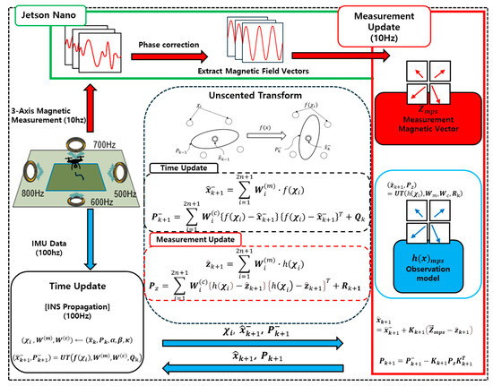
Figure 2. Structure of TC UKF.

As depicted in Figure 2, the IMU (Inertial Measurement Unit) data are measured at 100 Hz, while the Magnetic Field Vector data are measured at 10 Hz. If the synchronization between the IMU and Magnetic Field Vector is not aligned, the navigation process is performed using INS propagation based solely on the IMU. During this process, both the state estimate and error covariance estimate are computed. The moment when the IMU and MPS become synchronized is referred to as the measurement update phase. At this stage, the extracted magnetic vector is used to obtain measurement values, and the observation model $h\left(\mathit{x}\right)$ is applied to derive the model-based magnetic field values using the state estimate. These values are then utilized to update the state, as well as the error covariance estimate.

The middle section of the figure illustrates the Unscented Transformation (UT), depicting the calculation of state estimates and error covariance estimates during both the time update and measurement update steps. The detailed mathematical formulation of this process is provided in Equations (9)–(26).

The navigation state is defined as shown in Equation (9).

$${\widehat{\mathit{x}}}_k={\left[\begin{array}{l}{\widehat{\mathit{p}}}_k\\ {\widehat{\mathit{v}}}_k\\ {\widehat{\mathit{q}}}_k\\ {\widehat{\mathit{b}}}_{acc,k}\\ {\widehat{\mathit{b}}}_{gyro,k}\end{array}\right]}_{16\times 1}$$

(9)

${\widehat{\mathit{p}}}_k$ represents the position in the $n$-frame, ${\widehat{\mathit{v}}}_k$ denotes the velocity in the $n$-frame, and ${\widehat{\mathit{q}}}_k$ represents the attitude expressed as a quaternion. ${\widehat{\mathit{b}}}_{acc,k}$ and ${\widehat{\mathit{b}}}_{gyro,k}$ correspond to the biases of the accelerometer and gyroscope, respectively. In the INS model $f\left(\mathit{x}\right)$, the position, velocity, acceleration, attitude, ${\mathit{b}}_{acc}$, and ${\mathit{b}}_{gyro}$ are updated as described in Equation (10).

$$\begin{gathered} {\mathit{p}}_{k+1}^{-}={\mathit{p}}_{\mathit{k}}+{\mathit{v}}_k·dt+0.5{\mathit{a}}_n·dt \\ {\mathit{v}}_{k+1}^{-}={\mathit{v}}_k+{\mathit{a}}_n·dt \\ {\mathit{b}}_{acc,k+1}^{-}={\mathit{b}}_{acc,k},\hspace{1em}\hspace{1em}{\mathit{b}}_{gyro,k+1}^{-}={\mathit{b}}_{gyro,k} \\ {\mathit{q}}_{k+1}^{-}={\mathit{q}}_k⨂{\mathit{q}}_w \end{gathered}$$

(10)

In this process, acceleration ${\mathit{a}}_n$ is given as described in Equation (11):

$${\mathit{a}}_n={\mathit{C}}_b^n·\left({\mathit{A}}_b-{\mathit{b}}_{acc,k}\right)-\left[0 0-{\mathit{g}}_n\right]$$

(11)

where ${\mathit{C}}_b^n$ represents the DCM, which defines the transformation from the body frame (b-frame) to the navigation frame. ${\mathit{A}}_b$ represents the acceleration in the b-frame and ${\mathit{g}}_n$ represents gravity. ${\mathit{q}}_w$ represents the quaternion-based attitude estimated from the gyroscope.

During the UT process, including the addition, scaling, and propagation of sigma points, the constraint that the quaternion norm must remain equal to 1 can be violated, leading to inaccuracies in attitude estimation [20,21]. To address this issue, this study converts quaternions into rotation vectors for the UT process:

$${\left(\sqrt{\left(n+\lambda \right){\mathit{P}}_k}\right)}_i={\left[\begin{array}{l}\delta {\widehat{\mathit{p}}}_{k,i}\\ \delta {\widehat{\mathit{v}}}_{k,i}\\ {\delta \widehat{\mathit{\varphi }}}_{k,i}\\ \delta {\widehat{\mathit{b}}}_{acc,k,i}\\ \delta {\widehat{\mathit{b}}}_{gyro,k,i}\end{array}\right]}_{15\times 1}$$

(12)

$${\mathit{\chi }}_i={\left[\begin{array}{l}{\widehat{\mathit{p}}}_k+\delta {\mathit{p}}_{k,i}\\ {\widehat{\mathit{v}}}_k+\delta {\widehat{\mathit{v}}}_{k,i}\\ \left.{{\widehat{\mathit{q}}}_k\left(\widehat{\mathit{\varphi }}\right.}_k,\delta {\widehat{\mathit{\varphi }}}_{k,i},+\right)\\ {\widehat{\mathit{b}}}_{acc,k}+\delta {\widehat{\mathit{b}}}_{acc,k,i}\\ {\widehat{\mathit{b}}}_{gyro,k}+\delta {\widehat{\mathit{b}}}_{gyro,k,i}\end{array}\right]}_{16\times 1},{\mathit{\chi }}_{i+n+1}={\left[\begin{array}{c}{\widehat{\mathit{p}}}_k-\delta {\widehat{\mathit{p}}}_{k,i}\\ {\widehat{\mathit{v}}}_k-\delta {\widehat{\mathit{v}}}_{k,i}\\ {\widehat{\mathit{q}}}_k\left({\widehat{\mathit{\varphi }}}_k,\delta {\widehat{\mathit{\varphi }}}_{k,i},-\right)\\ {\widehat{\mathit{b}}}_{acc,k}-\delta {\widehat{\mathit{b}}}_{acc,k,i}\\ {\widehat{\mathit{b}}}_{gyro,k}-\delta {\widehat{\mathit{b}}}_{gyro,k,i}\end{array}\right]}_{16\times 1}$$

(13)

where $i,n$, $\lambda$, $\widehat{\mathit{q}}({\widehat{\mathit{\varphi }}}_{k-1},\delta {\widehat{\mathit{\varphi }}}_{k-1,i},+)$, $\widehat{\mathit{q}}({\widehat{\mathit{\varphi }}}_{k-1},\delta {\widehat{\mathit{\varphi }}}_{k-1,i},-)$ is:

$$i=1,\dots ,n,\hspace{1em}\hspace{1em}n=15,\hspace{1em}\hspace{1em}\lambda ={\alpha }^2\left(n+\kappa \right)-n$$

(14)

$$\widehat{\mathit{q}}\left({\widehat{\mathit{\varphi }}}_k,\delta {\widehat{\mathit{\varphi }}}_{k, i},+\right)={\left[\begin{array}{c}\cos \left(0.5‖{\widehat{\mathit{\varphi }}}_k+\delta {\widehat{\mathit{\varphi }}}_{k, i}‖\right)\\ \sin \left(0.5‖{\widehat{\mathit{\varphi }}}_k+\delta {\widehat{\mathit{\varphi }}}_{k, i}‖\right)·{\displaystyle \frac{{(\widehat{\mathit{\varphi }}}_k+\delta {\widehat{\mathit{\varphi }}}_{k, i})}{‖{(\widehat{\mathit{\varphi }}}_k+\delta {\widehat{\mathit{\varphi }}}_{k, i})‖}}\end{array}\right]}_{4\times 1}$$

(15)

$$\widehat{\mathit{q}}\left({\widehat{\mathit{\varphi }}}_k,\delta {\widehat{\mathit{\varphi }}}_{k, i},-\right)={\left[\begin{array}{c}\cos \left(0.5‖{\widehat{\mathit{\varphi }}}_k-\delta {\widehat{\mathit{\varphi }}}_{k, i}‖\right)\\ \sin \left(0.5‖{\widehat{\mathit{\varphi }}}_k-\delta {\widehat{\mathit{\varphi }}}_{k, i}‖\right)·{\displaystyle \frac{{(\widehat{\mathit{\varphi }}}_k-\delta {\widehat{\mathit{\varphi }}}_{k, i})}{‖{(\widehat{\mathit{\varphi }}}_k-\delta {\widehat{\mathit{\varphi }}}_{k, i})‖}}\end{array}\right]}_{4\times 1}$$

(16)

In Equation (14), $n$ represents the system order, while $\alpha$ and $\kappa$ denote the hyperparameters of the UKF. $\widehat{\mathit{q}}\left({\widehat{\mathit{\varphi }}}_k,\delta {\widehat{\mathit{\varphi }}}_{k, i},+\right)$ and $\widehat{\mathit{q}}\left({\widehat{\mathit{\varphi }}}_k,\delta {\widehat{\mathit{\varphi }}}_{k, i},-\right)$ represent the attitude estimated using the rotation vector, expressed in quaternion form.

In the time update, the state estimate ${\widehat{\mathit{x}}}_{k+1}^{-}$ and error covariance ${\mathit{P}}_{k+1}^{-}$ are calculated as shown in Equations (17) and (18). In this case, $f\left(\mathit{x}\right)$, expressed in Equation (17) corresponds to the INS model presented in Equation (10). ${\mathit{Q}}_k$ represents system noise covariance.

$${\widehat{\mathit{x}}}_{k+1}^{-}=W_i^{\left(m\right)}{\displaystyle \sum _{i=1}^{2n+1}}f\left({\mathit{\chi }}_i\right)$$

(17)

$${\mathit{P}}_{k+1}^{-}=W_i^{\left(c\right)}{\displaystyle \sum _{i=1}^{2n+1}}\left.\{f\left({\mathit{\chi }}_i\right)-{\widehat{\mathit{x}}}_{k+1}^{-}\right\}{\left.\{f\left({\mathit{\chi }}_i\right)-{\widehat{\mathit{x}}}_{k+1}^{-}\right\}}^T+{\mathit{Q}}_k$$

(18)

During the measurement update, the previously calculated $\mathit{\chi }$ is applied to the observation model to compute the measurements ${\widehat{\mathit{z}}}_{k+1}$ and covariance ${\mathit{P}}_z,{\mathit{P}}_{xz}$, as shown in Equations (19)–(21). ${\mathit{R}}_{k+1}$ represents measurement noise covariance. In this study, the design of the measurement noise covariance is based on Reference [5], ensuring that it is proportional to the square of the measurement magnitude.

$${\widehat{\mathit{z}}}_{k+1}=W_i^{\left(m\right)}\sum _{i=1}^{2n+1}h\left({\mathit{\chi }}_i\right)$$

(19)

$${\mathit{P}}_z=W_i^{\left(c\right)}\sum _{i=1}^{2n+1}\left.\{h\left({\mathit{\chi }}_i\right)-{\widehat{\mathit{z}}}_{k+1}\right\}{\left.\{h\left({\mathit{\chi }}_i\right)-{\widehat{\mathit{z}}}_{k+1}\right\}}^T+{\mathit{R}}_{k+1}$$

(20)

$${\mathit{P}}_{xz}=W_i^{\left(c\right)}\sum _{i=1}^{2n+1}\left\{{\mathit{\chi }}_i-{\widehat{\mathit{x}}}_{k+1}^{-}\right\}{\left.\{h\left({\mathit{\chi }}_i\right)-{\widehat{\mathit{z}}}_{k+1}\right\}}^T$$

(21)

where $W_i^{\left(m\right)}$ and $W_i^{\left(c\right)}$ is:

$$W_1^{\left(m\right)}={\displaystyle \frac{\lambda }{\left(n+\lambda \right)}}, W_1^{\left(c\right)}={\displaystyle \frac{\lambda }{\left(n+\lambda \right)}}+\left(1-{\alpha }^2+\beta \right)$$

(22)

$$W_i^{\left(m\right)}=W_i^{\left(c\right)}={\displaystyle \frac{1}{2\left(n+\lambda \right)}}$$

(23)

In Equation (20), ${\mathit{P}}_{\mathit{z}}$ represents the measurement innovation covariance, while in Equation (21), ${\mathit{P}}_{\mathit{x}\mathit{z}}$ denotes the cross-covariance between the state and the measurement. The weights $W_i^{\left(m\right)}$ and $W_i^{\left(c\right)}$, defined in Equations (22) and (23), correspond to the weighting factors for the state estimate and the covariance calculation, respectively. In Equation (22), $\beta$ in $W_1^{\left(c\right)}$ represents a hyperparameter of the UKF.

Using this, the Kalman gain ${\mathit{K}}_{k+1}$ is calculated as shown in Equation (24), and the state ${\widehat{\mathit{x}}}_{k+1}$ and error covariance ${\mathit{P}}_{k+1}$ are updated as shown in Equations (25) and (26). At this point, $\mathit{Z}$ in Equation (25) represents the measurement values.

$${\mathit{K}}_{k+1}={\mathit{P}}_{xz}{\left({\mathit{P}}_z\right)}^{-1}$$

(24)

$$\begin{array}{c}{\widehat{\mathit{x}}}_{k+1}={\widehat{\mathit{x}}}_{k+1}^{-}+{\mathit{K}}_{k+1}\left(\mathit{Z}-{\widehat{\mathit{z}}}_{k+1}\right)\end{array}$$

(25)

$${\mathit{P}}_{k+1}={\mathit{P}}_{k+1}^{-}-{\mathit{K}}_{k+1}{\mathit{P}}_z{\mathit{K}}_{k+1}^T$$

(26)

2.2. Estimation of UKF Hyperparameters Using the SIR Process

The hyperparameters of the traditional UKF, namely alpha $\left(\alpha \right)$, beta ($\beta$), and kappa $\left(\kappa \right)$, play a role in controlling the distribution of the sigma point region. Specifically, $\alpha$ is typically set between 0.001 and 1, $\kappa$ is set to 0 or $3-n$ when $n$ is less than 3 [14,15], and $\beta$ is optimally set to 2 under Gaussian distribution assumptions [13]. However, these predefined values are not always optimal, leading to numerous studies aimed at identifying the best hyperparameter settings [16,17,18,19].

Unlike prior studies that directly estimated these parameters, this study utilizes the weights derived from the SIR process in the Particle Filter to determine the optimal hyperparameters. Through the SIR process, the hyperparameter values are not fixed, but instead adjusted to reflect regions of increased model uncertainty or repeated uncertainty. This adaptability allows for improved navigation results. The PDF (Probability Density Function) used for this calculation process is constructed as shown in Algorithm 1:

Algorithm 1: PDF Calculation

1: Compute the Probability Density Function (PDF) for measurement update in SIR-UKF:$\hspace{1em}\hspace{1em}\hspace{1em}\hspace{1em}\hspace{1em}\hspace{1em}p\left({\mathit{z}}_k|{\mathit{x}}_k\right)={\displaystyle \frac{1}{\sqrt{{\left(2\pi \right)}^n \mathrm{d}\mathrm{e}\mathrm{t}\left(\mathit{R}\right)}}}\mathrm{e}\mathrm{x}\mathrm{p}\left(-0.5{\left({\mathit{Z}}_k-h\left({\mathit{x}}_k\right)\right)}^T{\mathit{R}}^{-1}\left({\mathit{Z}}_k-h\left({\mathit{x}}_k\right)\right)\right)$ 2: Return the computed $p\left({\mathit{z}}_k|{\mathit{x}}_k\right)$

The terms are defined as follows: ${\mathit{Z}}_k$: Measurement at time $k$; ${\mathit{x}}_k$: State at time $k$; $h\left({\mathit{x}}_k\right)$: Observation model at time $k$ based on the state; $\mathit{R}$: Measurement noise covariance matrix.

Using Algorithm 1, the PDF value can be computed for the measured magnetic field ${\mathit{Z}}_k$ and the model-derived magnetic field vector $h\left({\mathit{x}}_k\right)$. This allows the model-based magnetic field vector, computed from the currently estimated state, to have a higher PDF value when it closely matches the actual measured magnetic field.

The SUKF (SIR-UKF) process is shown in Algorithm 2:

Algorithm 2: SIR-UKF
1:	for	$IMU Time=1 to Experiment end$do
2:		$\mathbf{S}\mathbf{t}\mathbf{e}\mathbf{p} 1:$ Distribute hyperparameter
3:		$Hyperparameter:$ $(\alpha \leftarrow 0.1 ~0.15, \beta \leftarrow 2~20, \kappa \leftarrow 0~18)$$point \leftarrow length (Number of Hyperparameters)$
4:		$\mathbf{S}\mathbf{t}\mathbf{e}\mathbf{p} 2:$ Start UT using distributed $\alpha , \beta , \kappa$
5:		for	$i=1 to point$do
6:			$state \leftarrow UT \left(Each of \alpha , \beta , \kappa is applied individually\right)$
7:			$\mathbf{S}\mathbf{t}\mathbf{e}\mathbf{p} 3:$ Check the Measurement Synchronization (Sync)
8:			if	$IMU Sync\ne Measurement Sync$then
9:				$weight \leftarrow {\displaystyle \frac{1}{point}}$
10:			else
11:				Calculate $PDF$ using Measurement and Observation model $h\left(x\right)$
12:				$weight\propto weight\times PDF$
13:				if	$i=point$then
14:					$weight={\displaystyle \frac{weight}{\sum weight}}$
15:				end if
16:			end if
17:		end for
18:		$\mathbf{S}\mathbf{t}\mathbf{e}\mathbf{p} 4:$ Resampling and save hyperparameter
19:		Go back to$\mathbf{S}\mathbf{t}\mathbf{e}\mathbf{p} 1$
20:	end for

The process of Algorithm 2 can be described as follows. Step 1: the current state is set to the $k$-th iteration, and the hyperparameters are initialized within a predefined range to ensure appropriate distribution. Step 2: the UT process is performed using the distributed hyperparameters. This process is repeated as many times as the number of distributed hyperparameters. Step 3: the synchronization between the IMU data and measurement values is verified. If synchronization is not achieved, the weights are uniformly assigned as ${\displaystyle \frac{1}{point}}$. If synchronization is achieved, the PDF value is computed using Algorithm 1, and the weights are adjusted so that data with higher PDF values receive greater weights. Once the process is repeated for the specified number of points, the weights are normalized. Step 4: resampling is performed based on the calculated weights, ensuring that the hyperparameters with higher PDF values exert a greater influence. The obtained hyperparameters are stored, and the process restarts from Step 1 for the k + 1-th iteration. This process is conducted based on post-processing data.

3. Magnetic Vector Error Analysis During Flight

3.1. Experimental Environment

This section describes the experimental environment and scenarios. Figure 3a illustrates the experimental environment, including the coil arrangement and a 6 m spacing between the coils. Figure 3b depicts the components of the drone, which is equipped with a mission computer, the Jetson Nano, operating in an Ubuntu 18.04 environment, and a Pixhawk Hex Cube Black for drone flight. A receiver for collecting magnetic vectors is mounted on the underside of the drone. The receiver is equipped with a magnetometer sensor consisting of HMC1001 and HMC1002, while the IMU used is the ADIS16500.

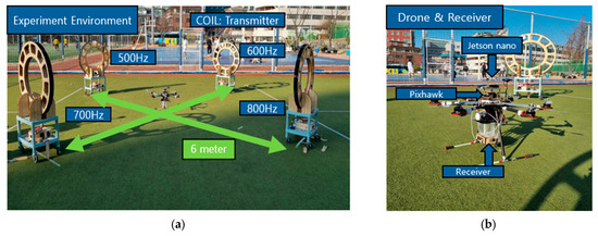
Figure 3. (a) Outdoor experimental environment. (b) Drone components.

For the flight experiment, the GPS-RTK (Global Positioning System Real-Time Kinematic) mode provided by Pixhawk, which offers an accuracy level of 2–3 cm, is used as the reference system. At the start of the experiment, magnetic vectors from the receiver and IMU data were transmitted to the main computer via UART (Universal Asynchronous Receiver/Transmitter), while the RTK (Real-Time Kinematic) information from Pixhawk was simultaneously transmitted to the main computer via MAVROS. The transmitted data were stored in a ROS1 environment and subsequently used to analyze the flight results. Previous studies have shown that the distortion of magnetic fields caused by eddy currents is significantly reduced in outdoor environments. Based on this, the experiment was conducted in an outdoor environment to evaluate the performance of a navigation method that performs 3D magnetic field navigation using pure magnetic vectors, which we refer to as the MPS 3D LS.

3.2. Experimental Details

This section describes the data configuration used to validate the effectiveness of the proposed algorithm. For the drone flight, the manual mode was utilized, with the flight controlled via a remote controller.

3.2.1. Data with Rapidly Increasing Model Uncertainty

This section explains the data related to the rapidly increasing errors between magnetic field measurements and model values. The flight trajectory follows a rectangular path toward 500, 600, 800, and 700 Hz in sequence, with continuous altitude changes during the flight. Data from the flight segment between 10 and 85 s were analyzed. To compute the magnetic field model values, the navigation solution from the Pixhawk RTK was used as reference data. Figure 4a illustrates the errors for each coil and the discrepancies between the measured and modeled magnetic fields along the x, y, and z axes. Breaking down the actual flight segment, the drone passed near the 500 Hz coil around 20 s, the 600 Hz coil around 30 s, the 800 Hz coil between 35 and 45 s, and the 700 Hz coil around 50 s. During the actual flight, the wind conditions caused the drone to remain near the 800 Hz coil for an extended period, which highlighted the model’s uncertainty in that region. Figure 4b displays the aggregated errors from all coils along each axis. Analyzing this graph shows that before approaching the 800 Hz coil, the model’s uncertainty increases gradually without steep slopes. However, near the 800 Hz coil, the error values rise sharply. A detailed comparison of the navigation solutions within this segment will be presented in the next section.

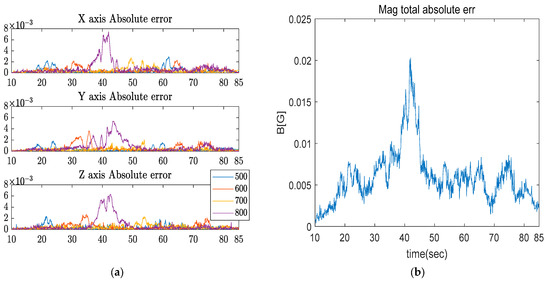
Figure 4. (a) Absolute error values. (b) Total sum of absolute errors.

3.2.2. Data with Repeated Model Uncertainty

This section describes the error data between magnetic field measurements and model values where model uncertainty repeatedly occurs. The flight trajectory involved continuous altitude changes centered at a specific location, and data from the flight segment between 15 and 80 s were analyzed. Using the same method as in Section 3.2.1, the absolute error between the magnetic field measurements and model values was calculated. Graphs showing the errors for each axis are presented in Figure 5a, while the aggregated error data are shown in Figure 5b. Unlike the data in Section 3.2.1, these data exhibit rapidly fluctuating error values over time. The resulting gradual performance differences in the filter will be analyzed in detail in the next section.

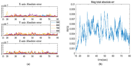
Figure 5. (a) Absolute error values. (b) Total sum of absolute errors.

4. Navigation Results

4.1. Experiment Results

4.1.1. Results for Data with Rapidly Increasing Model Uncertainty (Set 1)

The rectangular flight trajectory with increasing model uncertainty due to altitude changes is shown in Figure 6, and the position and attitude errors are shown in Figure 7. As previously mentioned, the flight was conducted in the order of 500, 600, 800, and 700 Hz, with continuous altitude variations during the flight.

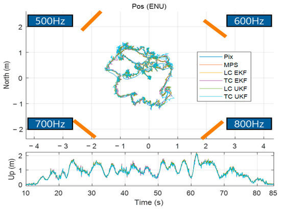
Figure 6. Rectangular trajectory with altitude changes.

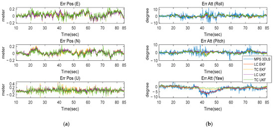
Figure 7. (a) Position error graphs. (b) Attitude error graphs.

In Figure 7, the error graphs reveal that during a 40 s interval of increasing model uncertainty, there is no significant difference in the positional results among the fusion methods. However, a sharp increase in error is observed in the yaw angle. This can be attributed to the distortion of magnetic vectors and increased model uncertainty, as explained in Section 3. These factors degrade the performance of magnetic-based navigation (MPS 3D LS), particularly in attitude estimation, where nonlinearity is pronounced.

To evaluate the performance of the proposed TC UKF, this study compares the results of Loosely Coupled EKFs and UKFs with those of a Tightly Coupled EKF. The EKF and UKF differ in their approach to estimating the error covariance. While the UKF employs the Unscented Transformation (UT) to estimate the error covariance, the EKF utilizes the Jacobian of the state for computation. In the Loosely Coupled MPS-INS method, the position and attitude computed from Equations (7) and (8) during the measurement update process are used as measurements for integration with the INS. Consequently, Loosely Coupled filters that directly utilize the MPS 3D LS results during the measurement update process reflect the position and attitude derived from the distorted MPS 3D LS navigation output. As a result, the navigation performance of the Loosely Coupled approach deteriorates. In contrast, the Tightly Coupled approach does not use the distorted MPS 3D LS navigation results during the measurement update process, but instead directly utilizes the magnetic vector itself. Thus, the Tightly Coupled filter demonstrates greater robustness compared to the MPS 3D LS and the Loosely Coupled EKF and UKF. In particular, the proposed TC UKF outperforms the conventional TC EKF in terms of yaw estimation accuracy.

The segments for navigation analysis are divided as shown in Figure 8, and the navigation results are presented in Table 1.

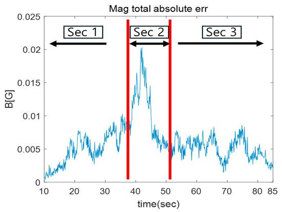
Figure 8. Segments for data analysis with rapidly increasing model uncertainty (Set 1).

Table 1. Results for data with rapidly increasing model uncertainty.

Set 1	Navigation Method	Position RMSE [Centimeter]				Attitude RMSE [Deg]
		East	North	Up	3D	Roll	Pitch	Yaw	3D
Sec 1	MPS 3D LS	5.43	4.63	6.55	9.69	2.00	2.17	1.49	3.30
	LC EKF	5.69	4.95	7.92	10.93	1.04	1.07	0.93	1.76
	LC UKF	5.92	5.10	8.06	11.22	1.12	1.00	0.84	1.72
	TC EKF	6.44	5.23	8.93	12.19	1.03	1.09	1.05	1.83
	TC UKF	4.99	7.27	7.51	11.58	1.21	1.04	0.85	1.81
Sec 2	MPS 3D LS	5.84	6.14	8.15	11.75	4.16	2.44	5.62	7.41
	LC EKF	6.25	6.35	9.65	13.14	1.86	1.16	5.37	5.80
	LC UKF	6.43	6.58	9.81	13.45	1.73	1.11	4.85	5.27
	TC EKF	4.83	6.15	12.19	14.48	1.88	1.28	2.50	3.38
	TC UKF	5.46	5.95	10.05	12.90	2.15	1.76	1.29	3.07
Sec 3	MPS 3D LS	5.28	7.89	6.42	11.46	2.11	2.25	2.12	3.74
	LC EKF	6.17	8.42	8.24	13.29	1.16	1.15	1.72	2.37
	LC UKF	6.41	8.58	8.12	13.44	1.25	1.04	1.26	2.06
	TC EKF	6.75	8.97	8.56	14.11	1.22	1.16	1.64	2.35
	TC UKF	6.16	9.95	8.10	14.23	1.34	1.28	0.83	2.03
Total	MPS 3D LS	5.39	6.42	6.78	10.78	2.59	2.24	2.97	4.53
	LC EKF	5.95	6.81	8.33	12.30	1.31	1.11	2.68	3.78
	LC UKF	6.17	6.97	8.38	12.53	1.35	1.03	2.34	2.90
	TC EKF	6.23	7.13	9.43	13.36	1.32	1.15	1.65	2.41
	TC UKF	5.55	8.21	8.21	12.87	1.51	1.31	0.93	2.20

The analysis of Table 1 is as follows: Firstly, for Sec 1, similar results are observed across all fusion methods and filters. Examining the error graph for the Sec 1 region reveals that this segment does not exhibit a sharp increase in the absolute error, nor does it show repetitive fluctuations. This is because significant distortions of magnetic vectors or repeated model uncertainty are not observed in this region. As a result, there is no noticeable performance difference between Loosely Coupled (LC) and Tightly Coupled (TC) structure in this segment. The RMSE (Root Mean Squared Error) values, except for the MPS 3D LS, are almost identical. For the MPS 3D LS, while the position estimation is the most accurate, the attitude error is higher compared to the other fusion methods.

Secondly, for Sec 2, significant differences in the results are observed. In this segment, the steep slope of the error graph indicates a rapid increase in magnetic vector distortion and model uncertainty. As a result, the performance of the MPS 3D LS degrades significantly in terms of attitude estimation, due to the distortion of magnetic vectors. Filters based on the LC structure, which rely on these measurements, also exhibit poor attitude estimation results. In contrast, TC filters demonstrate greater robustness against distorted magnetic vector measurements, yielding better results compared to MPS 3D LS and LC methods. Additionally, as model uncertainty reaches its peak, the UKF outperforms the EKF in attitude estimation.

Thirdly, for Sec 3, the magnitude of the absolute error remains relatively constant and then decreases, without exhibiting repetitive fluctuations. As the filters converge based on the Sec 2 segment, the results indicate that the LC and TC approaches yield a nearly identical performance in terms of attitude estimation.

Finally, examining the results across the entire flight segment reveals that, in terms of position, the 3D Pos RMSE value of the MPS 3D LS is the best. However, its performance in attitude estimation is the worst. The position results of the other navigation methods, excluding the MPS 3D LS, are almost identical. Among these results, the TC UKF demonstrates the best performance in attitude estimation, showing the lowest 3D RMSE Attitude value. Analyzing the attitude error graph indicates that, in the Sec 2 segment, the MPS 3D LS and LC methods relying on its measurements exhibit large errors in yaw. However, TC filters show smaller errors in this segment, with the UKF outperforming the EKF in terms of attitude error values.

4.1.2. Results for Data with Repeated Model Uncertainty (Set 2)

The hovering flight trajectory with increasing model uncertainty due to altitude changes is shown in Figure 9, and the position and attitude errors are shown in Figure 10. This trajectory involves continuous altitude variations starting from the initial takeoff position.

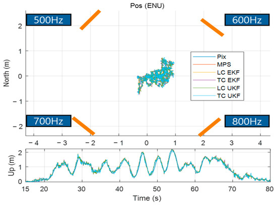
Figure 9. Hovering flight with altitude changes.

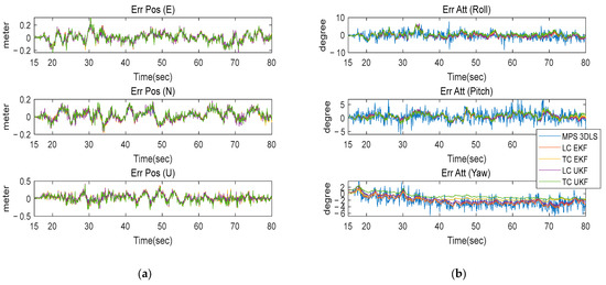
Figure 10. (a) Position error graphs. (b) Attitude error graphs.

In Figure 10, the error graph reveals an increasing trend in the yaw attitude error of the MPS 3D LS over time. This phenomenon is attributed to the distortion of model measurements and the repeated occurrence of model uncertainty, which gradually degrades the attitude estimation performance of the MPS 3D LS. As described in the Set 1 experiment, the performance of the LC EKF and LC UKF, which utilize the navigation results of the MPS 3D LS as measurements, also deteriorates. In contrast, the TC EKF and TC UKF demonstrate strong robustness against persistently distorted magnetic vectors and repeated model uncertainty. Furthermore, the Set 2 experiment results confirmed that the proposed TC UKF outperforms the conventional TC EKF in terms of yaw estimation accuracy.

The segments for navigation analysis are divided as shown in Figure 11, and the navigation results are presented in Table 2.

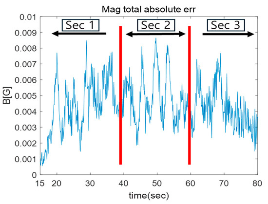
Figure 11. Segments for data analysis with repeated model uncertainty (Set 2).

Table 2. Results for data with repeated model uncertainty.

Set 2	Navigation Method	Position RMSE [Centimeter]				Attitude RMSE [Deg]
		East	North	Up	3D	Roll	Pitch	Yaw	3D
Sec 1	MPS 3D LS	4.68	6.59	7.81	11.24	1.96	1.88	1.92	3.33
	LC EKF	5.50	7.46	9.53	13.29	1.57	1.18	1.41	2.41
	LC UKF	5.65	7.50	9.53	13.38	1.75	1.22	1.12	2.41
	TC EKF	5.26	7.44	9.74	13.33	1.65	1.17	0.98	2.25
	TC UKF	5.81	7.91	9.74	13.83	1.70	1.14	0.95	2.25
Sec 2	MPS 3D LS	5.01	5.24	10.30	12.60	1.98	1.96	3.22	4.25
	LC EKF	5.47	6.08	11.66	14.25	1.15	1.16	2.95	3.37
	LC UKF	5.63	6.04	11.62	14.25	1.16	1.05	2.43	2.89
	TC EKF	5.60	5.82	11.76	14.27	1.14	1.16	1.76	2.40
	TC UKF	5.78	5.68	11.30	13.90	1.20	1.25	0.97	1.99
Sec 3	MPS 3D LS	5.83	6.83	5.66	10.62	2.09	2.20	3.35	4.52
	LC EKF	6.56	7.27	6.96	12.02	1.12	1.30	3.02	3.48
	LC UKF	6.78	7.61	7.38	12.58	1.14	1.27	2.59	3.10
	TC EKF	6.43	7.22	7.90	12.49	1.16	1.39	1.91	2.63
	TC UKF	6.77	7.68	7.86	12.91	1.04	1.51	1.44	2.34
Total	MPS 3D LS	5.08	6.16	8.22	11.46	2.01	1.99	2.87	4.03
	LC EKF	5.73	6.87	9.68	13.18	1.34	1.19	2.52	3.10
	LC UKF	5.91	6.98	9.73	13.35	1.42	1.17	2.10	2.79
	TC EKF	5.67	6.77	9.97	13.32	1.37	1.22	1.58	2.42
	TC UKF	6.02	7.05	9.79	13.48	1.37	1.29	1.13	2.19

The analysis of Table 2 is as follows: Firstly, for Sec 1, the distortion of measurements and the repetition of model uncertainty did not significantly affect the navigation results. As a result, the navigation outcomes in Sec 1, except for the MPS 3D LS, are nearly identical, with no substantial differences observed between the EKF and UKF. In this segment, the MPS 3D LS demonstrates the highest accuracy in terms of position. However, its performance in attitude estimation is considerably poor.

Secondly, for Sec 2, the persistent changes in magnetic distortion and model uncertainty have a significant impact on the navigation results. First, the results of the MPS 3D LS exhibit poorer attitude performance compared to Sec 1. Consequently, LC methods also demonstrate lower attitude estimation performance. In contrast, TC methods show greater robustness against continuous distortions, achieving better attitude performance than the MPS 3D LS and LC approaches. Additionally, due to the repetitive nature of model uncertainty, the attitude performance of navigation using the UKF is superior to that of the EKF.

Thirdly, for Sec 3, the persistent magnetic distortion and model uncertainty caused the filters to converge to the conditions of this segment. Among the three segments, the MPS 3D LS exhibited the lowest attitude performance in Sec 3, and the LC results based on it also showed poor attitude estimation performance. In contrast, TC methods demonstrated robustness against continuous magnetic distortions. Due to persistent model uncertainty, navigation solutions based on the UKF outperformed those based on the EKF.

Finally, examining the results across the entire flight segment reveals that, similarly to the first experiment, the MPS 3D LS demonstrates the best positional performance but the poorest attitude performance. Consequently, the TC approach shows better attitude performance than the LC approach for the same reasons. Given the repetitive nature of model uncertainty in this dataset, the UKF-based fusion method, which is more robust to model uncertainty, outperforms the EKF-based method in terms of attitude performance.

4.2. Comparison of Navigation Solutions Between Conventional UKF and SUKF

In the conventional UKF, the hyperparameters were set as $\alpha =0.1, \beta =2, \kappa =0$, or $\kappa =3-n$, depending on the value of $n,$ for calculation. Previous studies [14,16,17,18,19] have demonstrated that hyperparameters significantly affect UKF performance and that adjusting these parameters can enhance the filter’s performance. In this study, the TC UKF consistently demonstrated the best performance across all experimental datasets, and the results of applying the hyperparameters $(\alpha , \beta , \kappa )$ estimated through the SIR process to the TC UKF are as follows. Note that the hyperparameters can be computed online, yet an offline computation is applied due to the real-time computational limitation.

First, we present the results for the rectangular trajectory with altitude changes (Set 1). In the conventional UKF, the hyperparameters are set as $\alpha =0.1, \beta =2, \kappa =0$, whereas in the SUKF (SIR-UKF), the hyperparameters vary within the ranges $\alpha =0.1~0.15, \beta =2~20, \kappa =0~18$. In the case of Set 1, the hyperparameter values were determined using an empirically derived range obtained via experiments. Table 3 presents the navigation results of the UKF and SUKF for Set 1.

Table 3. Comparison between conventional UKF and SUKF (Set 1).

Set1	Navigation Method	Position RMSE [Centimeter]				Attitude RMSE [Deg]
		East	North	Up	3D	Roll	Pitch	Yaw	3D
Sec 1	TC UKF	4.99	7.27	7.51	11.58	1.21	1.04	0.85	1.81
	TC SUKF	6.06	5.56	7.62	11.21	1.05	1.06	0.89	1.74
Sec 2	TC UKF	5.46	5.95	10.05	12.90	2.15	1.76	1.29	3.07
	TC SUKF	4.38	6.03	10.62	12.97	1.86	1.53	1.46	2.81
Sec 3	TC UKF	6.16	9.95	8.10	14.23	1.34	1.28	0.83	2.03
	TC SUKF	6.33	9.40	7.79	13.75	1.24	1.20	0.96	1.98
Total	TC UKF	5.55	8.21	8.21	12.87	1.51	1.31	0.93	2.20
	TC SUKF	5.82	7.42	8.27	12.54	1.34	1.22	1.04	2.09

Next, we present the results for the hovering trajectory with altitude changes (Set 2). Similarly, the UKF uses the same values for $\alpha , \beta$, and $\kappa$, and the SUKF adopts hyperparameters within the same criteria as Set 1. Table 4 presents the navigation results of the UKF and SUKF for Set 2.

Table 4. Comparison between conventional UKF and SUKF (Set 2).

Set 2	Navigation Method	Position RMSE [Centimeter]				Attitude RMSE [Deg]
		East	North	Up	3D	Roll	Pitch	Yaw	3D
Sec 1	TC UKF	5.81	7.91	9.74	13.83	1.70	1.14	0.95	2.25
	TC SUKF	5.32	7.39	9.43	13.10	1.62	1.10	0.99	2.19
Sec 2	TC UKF	5.78	5.68	11.30	13.90	1.20	1.25	0.97	1.99
	TC SUKF	5.62	5.64	11.17	13.72	1.20	1.22	1.01	1.98
Sec 3	TC UKF	6.77	7.68	7.86	12.91	1.04	1.51	1.44	2.34
	TC SUKF	6.51	7.41	7.60	12.45	1.07	1.44	1.50	2.33
Total	TC UKF	6.02	7.05	9.79	13.48	1.37	1.29	1.13	2.19
	TC SUKF	5.72	6.75	9.57	13.03	1.33	1.24	1.17	2.16

The proposed TC SUKF (Tightly Coupled SIR-UKF) demonstrated improved results compared to the conventional TC UKF, which had previously shown the best attitude performance across all datasets. The TC SUKF outperformed the TC UKF not only in attitude estimation, but also in positional accuracy. In Table 3, the TC SUKF exhibited better attitude results than the TC UKF, particularly in regions with the highest model uncertainty (Sec 2), despite showing millimeter-level differences in position compared to the TC UKF. Additionally, the proposed TC SUKF demonstrated superior performance over the TC UKF in datasets with abrupt increases in magnetic distortions and model uncertainties (Set 1), rather than in datasets with repetitive distortions and uncertainty (Set 2).

[Note] The improvement in performance primarily originates from the SIR process. As shown in Algorithm 1, the denominator of the Probability Density Function (PDF) calculation includes the measurement covariance $\mathit{R}$. This implies an inverse relationship between the magnitude of $\mathit{R}$ and the PDF value. Specifically, as model uncertainty increases, the measurement covariance $\mathit{R}$ grows larger, causing the PDF value to decrease accordingly. In scenarios where model uncertainty increases, the PDF values for data with high uncertainty decrease, leading to a reduction in their corresponding weights. Consequently, data with high uncertainty exert less influence during the resampling process. As a result, in regions of high uncertainty, hyperparameters with relatively lower uncertainty are predominantly resampled to maintain filter stability. Conversely, when model uncertainty decreases, the PDF value increases, leading to an increase in the weights associated with high-uncertainty data. This enables the filter to resample hyperparameters with greater uncertainty, enhancing its ability to handle higher uncertainty levels. In other words, as model uncertainty varies, the hyperparameters are dynamically adjusted, allowing the filter to effectively manage increased uncertainty and achieve more accurate state estimation.

5. Conclusions

This study analyzed the performance of magnetic navigation in a 6DoF drone environment and proposed a Tightly Coupled MPS-INS UKF integration method. Additionally, the effectiveness of the hyperparameters estimated through the SIR process for the UKF was demonstrated. In the drone flight environment, the MPS 3D LS showed a positional error of approximately 10 cm in terms of 3D RMSE Pos, exhibiting a performance advantage of less than 2 cm compared to other fusion methods. However, due to measurement distortions, the attitude error was approximately 4 degrees in terms of 3D RMSE Attitude, and increased to 7.4 degrees in regions with the highest model uncertainty. The results also demonstrated a decline in attitude estimation performance for the previously proposed EKF due to repetitive or rapidly increasing model uncertainty. The proposed UKF-based Tightly Coupled algorithm exhibited superior attitude performance in 3D flight environments and achieved the most robust attitude estimation results in datasets with significant model uncertainty. Furthermore, the UKF using hyperparameters estimated through the SIR process outperformed the conventional UKF with preset hyperparameters, delivering better positional and attitude results in datasets with increasing model uncertainty. Moreover, the proposed technique can be generalized for the continuous tracking of objects located behind obstacles or non-visible elements in the propagation medium—such as water, walls, or floors—by penetrating these barriers. Owing to its rapid provision of highly accurate continuous position and attitude estimates, this technique can be applied as a navigation method for the real-time precision control of unmanned vehicles.

References

- Blankenbach, J.; Norrdine, A. Position estimation using artificial generated magnetic fields. In Proceedings of the 2010 International Conference on Indoor Positioning and Indoor Navigation, Zurich, Switzerland, 15–17 September 2010; pp. 1–5. [Google Scholar] [CrossRef]
- Blankenbach, J.; Norrdine, A.; Hellmers, H. A robust and precise 3D indoor positioning system for harsh environments. In Proceedings of the 2012 International Conference on Indoor Positioning and Indoor Navigation (IPIN), Sydney, NSW, Australia, 13–15 November 2012; pp. 1–8. [Google Scholar] [CrossRef]
- Lee, B.; Cho, S.Y.; Lee, J.; Sung, S. Magneto-Inertial Integrated Navigation System Design Incorporating Mapping and Localization Using Concurrent AC Magnetic Measurements. IEEE Access 2019, 7, 131221–131233. [Google Scholar] [CrossRef]
- Pasku, V.; De Angelis, A.; De Angelis, G.; Arumugam, D.D.; Dionigi, M.; Carbone, P.; Moschitta, A.; Ricketts, D.S. Magnetic Field-Based Positioning Systems. IEEE Commun. Surv. Tutor. 2017, 19, 2003–2017. [Google Scholar] [CrossRef]
- Lee, B.; Bae, J.Y.; Lee, J.; Sung, S. Tightly Coupled Integration Design for a Magneto-Inertial Navigation System Using Concurrent AC Magnetic Measurements. IEEE Access 2020, 8, 76253–76266. [Google Scholar] [CrossRef]
- Lee, B.; Sung, S. Planar Pose Estimation System Design via Explicit Spatial Representation Model of Concurrent AC Magnetic Fields. IEEE Trans. Instrum. Meas. 2022, 71, 18505914. [Google Scholar] [CrossRef]
- Lee, B.; Lee, J.; Sung, S. Comparative Performance Analysis of AC Magnetic Positioning Algorithms With Realtime Implementation Environment. Int. J. Control Autom. Syst. 2024, 22, 265–275. [Google Scholar] [CrossRef]
- Yun, J.H.; Sung, S. Design of Range/IMU-Aided Integrated Magnetic Positioning System for Improving Vertical Pose Estimation Performance. Int. J. Aeronaut. Space Sci. 2023, 24, 1430–1442. [Google Scholar] [CrossRef]
- Kwon, D.; Lee, B.; Sung, S. Design and Performance Validation of Tightly Coupled Magneto-Inertial Navigation System for Robust Outdoor Application. IEEE Access 2024, 12, 142215–142226. [Google Scholar] [CrossRef]
- Kwon, D.; Seo, J.; Lee, B.; Sung, S. Magnetic-Inertial Odometry Design Using Artificial AC Magnetic Fields in Outdoor Environment. In Proceedings of the 2024 IEEE International Conference on Multisensor Fusion and Integration for Intelligent Systems (MFI), Pilsen, Czech Republic, 4–6 September 2024; pp. 1–6. [Google Scholar] [CrossRef]
- Julier, S.J.; Uhlmann, J.K.; Durrant-Whyte, H.F. A new approach for filtering nonlinear systems. In Proceedings of the 1995 American Control Conference—ACC’95, Seattle, WA, USA, 21–23 June 1995; Volume 3, pp. 1628–1632. [Google Scholar] [CrossRef]
- Julier, S.J.; Uhlmann, J.K. Unscented filtering and nonlinear estimation. Proc. IEEE 2004, 92, 401–422. [Google Scholar] [CrossRef]
- Wan, E.A.; Van Der Merwe, R. The unscented Kalman filter for nonlinear estimation. In Proceedings of the IEEE 2000 Adaptive Systems for Signal Processing, Communications, and Control Symposium (Cat. No.00EX373), Lake Louise, AB, Canada, 4 October 2000; pp. 153–158. [Google Scholar] [CrossRef]
- Julier, S.; Uhlmann, J.; Durrant-Whyte, H.F. A new method for the nonlinear transformation of means and covariances in filters and estimators. IEEE Trans. Autom. Control. 2000, 45, 477–482. [Google Scholar] [CrossRef]
- Julier, S.J. The scaled unscented transformation. In Proceedings of the 2002 American Control Conference (IEEE Cat. No.CH37301), Anchorage, AK, USA, 8–10 May 2002; Volume 6, pp. 4555–4559. [Google Scholar] [CrossRef]
- Straka, O.; Dunik, J.; Simandl, M. Scaling parameter in unscented transform: Analysis and specification. In Proceedings of the 2012 American Control Conference (ACC), Montreal, QC, Canada, 27–29 June 2012; pp. 5550–5555. [Google Scholar] [CrossRef]
- Scardua, L.A.; da Cruz, J.J. Complete offline tuning of the unscented Kalman filter. Automatica 2017, 80, 54–61. [Google Scholar] [CrossRef]
- Nielsen, K.; Svahn, C.; Rodriguez-Deniz, H.; Hendeby, G. UKF Parameter Tuning for Local Variation Smoothing. In Proceedings of the 2021 IEEE International Conference on Multisensor Fusion and Integration for Intelligent Systems (MFI), Karlsruhe, Germany, 23–25 September 2021; pp. 1–8. [Google Scholar] [CrossRef]
- Sakai, A.; Kuroda, Y. Discriminative Parameter Training of Unscented Kalman Filter. IFAC Proc. Vol. 2010, 43, 677–682. [Google Scholar] [CrossRef]
- Xia, G.; Wang, G. INS/GNSS Tightly-Coupled Integration Using Quaternion-Based AUPF for USV. Sensors 2016, 16, 1215. [Google Scholar] [CrossRef] [PubMed]
- Yang, Y.; Zhou, J.; Loffeld, O. Quaternion-based Kalman filtering on INS/GPS. In Proceedings of the 2012 15th International Conference on Information Fusion, Singapore, 9–12 July 2012; pp. 511–518. [Google Scholar]
Disclaimer/Publisher’s Note: The statements, opinions and data contained in all publications are solely those of the individual author(s) and contributor(s) and not of MDPI and/or the editor(s). MDPI and/or the editor(s) disclaim responsibility for any injury to people or property resulting from any ideas, methods, instructions or products referred to in the content. |
© 2025 by the authors. Licensee MDPI, Basel, Switzerland. This article is an open access article distributed under the terms and conditions of the Creative Commons Attribution (CC BY) license (https://creativecommons.org/licenses/by/4.0/).