Abstract
It is well known that mean elements obtained by canonical perturbation theory only agree partially with the average dynamics of the osculating orbit. While this fact does not necessarily compromise the accuracy of corresponding perturbation solutions, the loose use of the terminology “mean elements” in artificial satellite theory may obscure the understanding of the variety of available solutions in the literature, and thus make the implementation of additional patches to increase their performance ambiguous. We resort to noncanonical perturbation methods, and, for the main problem of artificial satellite theory (the -problem), compute the purely periodic, noncanonical, mean-to-osculating transformation that yields the exact separation between short- and long-period variations up to the second order of the zonal harmonic of the second degree. To our knowledge this transformation is new and was long-awaited by software developers in order to improve operational orbit propagation tools based on semianalytical integration. It is also shown that this kind of noncanonical solution confines the long-period oscillations of the semimajor axis in the mean variation equations.
1. Introduction
The decomposition of orbital motion into secular, long- and short-period effects allowed astronomers of the 18th and 19th centuries to better understand the dynamics of celestial objects, and, therefore, to make reasonably accurate predictions of their motions [1,2,3,4]. Analogous techniques were successfully applied to the prediction of orbits of artificial satellites since the beginning of the space era. In this task, the emphasis was placed on avoiding expansions of the elliptic functions so that the solutions may apply to the highly eccentric orbits typical of some artificial satellite missions [5,6,7].
The amplitudes of the fast, short-period fluctuations that modulate the long-term dynamics of artificial satellites and other celestial bodies are usually small. They are conveniently removed from the equations representing the dynamics by averaging techniques in order to more easily predict the slow variations of the “mean” orbital elements. The averaging is mathematically supported by a transformation from osculating to mean variables. But it happens that different changes of variables can be used to remove the short-period effects, a fact that makes the definition of mean elements non-unique, and even sometimes confusing [8]. Ideally, such kind of transformation should eliminate only the short-period effects—those related to the mean anomaly—so that the resulting mean elements capture all the effects that drive the long-term dynamics. This removal is easily accomplished when the mean anomaly appears explicitly in the variation equations. But this is not the case of artificial satellite theory, where the dependence of the variation equations on the mean anomaly remains implicit through the explicit appearance of the true or eccentric anomalies. The trouble, of course, can be solved by making the mean anomaly explicit, a procedure that requires carrying out expansions of the elliptic motion, and the consequent truncation of the series to some power of the eccentricity [9]. The good news is that efficient recursion formulas are available in the literature for the evaluation of these kinds of expansions [10]. However, the expansions constrain the range of the eccentricities to which the solution applies, on the one hand, and can result in very long trigonometric series [11,12], on the other hand, which may be bad news if dealing with highly eccentric orbits.
High-eccentricity orbits provide a variety of opportunities for satellite missions, and, therefore the elimination in closed form of the mean anomaly from the equations of the dynamics is clearly desired; it is also feasible—at least for usual perturbation models. But one should be aware that the closed form approach commonly hides the concomitant elimination of part of the long-period effects as a side effect of the procedure [13]. This unintended removal of some long-period terms from the mean elements dynamics is not at all of worry for analytical or semianalytical ephemeris computation, as far as they are recovered in the integration process. However, holding these terms in the mean-to-osculating transformation can certainly be a concern for some space geodesy applications. Indeed, the latter may require the exact separation of the short-period fluctuations from the long-term dynamics in order to obtain mean elements that strictly adhere to the average evolution of the osculating elements [14].
The exact decomposition of the orbital motion into short- and long-period effects is readily obtained with different perturbation techniques. Theoretically, the procedure is not difficult. It only requires the proper choice of the arbitrary integration functions of the slow variables which arise in the analytical computation of the mean-to-osculating transformation [15,16,17]. However, due to the definite and indefinite integrals that must be solved along the perturbation procedure, things may become a little involved in practice when the closed form is desired. Fortunately, most of the needed integrals have been previously reported in the literature, thus notably simplifying the task [3,18,19,20,21,22]. In spite of this decisive help, one should be aware that when the removal of short-period effects is approached with the popular canonical perturbation methods, the exact separation of short- and long-period effects is guaranteed only for the linear part of the mean-to-osculating transformation, beyond which Hamiltonian perturbation theory is no longer useful regarding this task [14,23].
First-order perturbation theories are in the roots of useful operational software dealing with real perturbation models. However, when approaching the propagation of circumterrestrial orbits, second-order effects of the Earth’s zonal harmonic of the second degree cannot be ignored in the implementation of the perturbation solution [24,25,26,27,28]. Closed-form expressions of these short-period, second-order terms have been known to the astrodynamics community for a long time. Yet, because they were computed with canonical perturbation methods, the higher-order terms of existing closed-form solutions of artificial satellite theory lack the exact separation between mean frequencies and purely periodic short-period corrections. To our knowledge, with the exception of simple toy models that are not suitable for dealing with the real dynamics [29], the literature lacks explicit expressions for the corresponding second-order terms of the mean-to-osculating transformation.
In this paper, we fill the gap and, for the main problem of artificial satellite theory (the -problem), compute in closed form of the eccentricity the second-order terms of the mean-to-osculating transformation that is purely periodic in the mean anomaly [30]. As expected, the obtained short-period corrections differ from the standard results obtained with canonical perturbation methods only in the long-period terms of second-order born by the latter. With the new mean-to-osculating transformation, the whole long-period effects of the dynamics are moved to the mean frequencies. Remarkably, the modifications in the equations of the long-term dynamics with respect to those obtained with Hamiltonian methods only affect the mean variation of the mean anomaly for a second-order theory. We also computed the third-order components of the mean dynamics. Because the mean variations are obtained based only on partial differentiation operations and averaging, their derivation adds little computational effort to the procedure. These higher-order terms of the mean dynamics show that the mean variation of the semimajor axis, which is null up to the second order of the long-term solution, no longer vanishes beyond this order. This feature is in clear contrast with the case of canonical perturbation methods, in which the removal of the mean anomaly from the Hamiltonian unavoidably yields the vanishing of the mean variation of the semimajor axis at any order.
In the process of deriving the third-order terms of the mean variations of the main problem, we confronted the closed-form integration of nontrivial functions whose dependence on the equation of the center deprives them of trigonometric character [31,32,33]. Still, we found that the solution of the required integrals can be approached by standard integration by parts. This conventional procedure reduces the problem to the integration of known functions of the elliptic motion whose solutions are either trivial or have been previously reported in the literature (refer to [20,21,22,34] and references therein).
In spite of the searched mean-to-osculating transformation being noncanonical by nature, the new perturbation theory has been computed in Delaunay canonical action-angle variables for simplicity, on the one hand, and with the aim of easing comparison with previous results in the literature, on the other hand. Undoubtedly, these variables bear clear drawbacks for operational purposes, mainly because of the lack of definition of the argument of the perigee of circular orbits. This geometrical singularity is manifested in the perturbation theory with the appearance of the small divisors problem. Not only does the evaluation of the perturbation solution in Delaunay variables break for exact circular orbits, but the expected convergence of the formal series in the limited time that they may remain valid is also clearly degraded in the case of low eccentricities.
Still, we do not see these limitations as a major concern since the utility of the closed form discussed in this paper is clearly tied to the high eccentricity of the propagated orbits. Otherwise, the customary expansions in powers of the eccentricity make it easy to replace the closed-form perturbation solution with the typical solution in nonsingular variables valid for the lower eccentricity orbits—whose construction only involves the solution of trivial integrals [11,35]. At the end, orbit-propagation suites commonly comprise different perturbation theories [36,37,38,39]. Moreover, because we derive the perturbation solution from a vectorial generating function [40,41,42], solving the perturbation problem in a different set of variables, for instance, nonsingular ones, does not require us to recompute the perturbation theory from scratch. On the contrary, it can be reformulated in the chosen variables from the computed generator in Delaunay variables, as is also the case with theories computed with canonical methods [11,43]. A reformulation of the closed-form solution in nonsingular variables is under development, and full details will be provided elsewhere when fully completed and tested.
The rest of the paper is organized as follows. In Section 2, we recall the basic formulation of the main problem, whose variation equations we arrange in a particular form that eases the desired closed-form integration. The perturbation solution is approached in Section 3. The technical details of the method are not discussed but instead, interested readers are just referred to the pertinent literature. The relevant equations of the solution are presented as far as their size allows to obtain dynamical insight from the printed expression. Still, those provided should be sufficient for a practitioner to replicate the theory and debug their own derivations. Differences of our noncanonical solution with a partner theory that does not impose the exact separation of the mean dynamics—which alternatively could have been computed by canonical methods—are illustrated in the short Section 4. Finally, the main differences between the different perturbation solutions of the main problem are illustrated in Section 5 for a significant example. We remark that this final section is not devoted to the validation of our codes, whose performance, for sure, would be greatly improved by software developers and specialists. On the contrary, we simply try to illustrate the dynamical differences between the different classes of perturbation solutions. That is why we feel satisfied with the insight provided by the chosen, single example.
2. The Main Problem of Artificial Satellite Theory
Constraining to the main part, the gravitational potential of the Earth at a point defined by the spherical coordinates , for geocentric distance, latitude, and longitude, respectively, is
where the physical parameters , R, and , denote the gravitational parameter, equatorial radius, and oblateness coefficient, respectively. The dynamical model represented by Equation (1) is customarily known as the main problem of artificial satellite theory [6]. Because the value of the Earth’s is very small, of the order of one thousandth, the solution to the main problem can be approached as a perturbation of the integrable Keplerian potential .
Finding approximate perturbation solutions to the main problem is suitably approached in Delaunay canonical variables , whose definition is commonly expressed in terms of the more familiar, noncanonical Keplerian variables as , , , , , and , where M denotes the mean anomaly, the argument of the perigee, the right ascension of the ascending node, a the orbit semimajor axis, e the eccentricity, and i the inclination with respect to the equatorial plane of the Earth. The sine of the latitude in Equation (1) is expressed in the orbital variables as , where is the argument of the latitude, with f denoting the true anomaly. In the same equation, the distance is written as the conic equation
where is the conic parameter, also known as the semilatus rectum.
The implicit dependence of the true anomaly on the mean one , which involves the solution of the Kepler equation, complicates the closed-form solution of the variation equations of the Delaunay variables stemming from the main problem potential (1). More precisely, the closed-form solution of the integrals that must be solved in the implementation of the perturbation approach is achieved after making a change in the integration variable. This change is based on the preservation of the angular momentum of the Keplerian motion . Then, in the fashion of [44], in preparation of the perturbation approach, the variation equations of the Delaunay osculating elements are written in the form
in which the perturbation functions , , are conveniently arranged as
where
is the Keplerian mean motion,
and the replacements and serve to abbreviate printed expressions. Needless to say that the Keplerian orbital elements and other variables displayed in the right sides of Equations (2)–(7) are functions of the Delaunay variables displayed in the left sides, whose particular forms are obtained from their corresponding definitions. Nonvanishing values of the eccentricity polynomials , , and are given in Table 1, whereas the inclination polynomials , and are presented in Table 2.

Table 1.
Eccentricity polynomials in Equations (8)–(12).
Table 2.
Inclination polynomials in Equations (8) and (9).
The Delaunay variables share the same deficiencies as the Keplerian elements, hence the appearance of the eccentricity in denominators of Equations (8) and (9). This geometric singularity for circular orbits is not essential; if desired, the offending denominators can be removed from the variation equations with the choice of different Keplerian sets of nonsingular variables [11,43,45,46].
The conservation of the third component of the angular momentum vector H stemming from the vanishing of Equation (7) decouples the variation in Equation (4) of the right ascension of the ascending node of the problem from the dynamics given by Equations (2), (3), (5) and (6). The latter comprise a reduced differential system of just two degrees of freedom. Therefore, the qualitative aspects of the decoupled dynamics can be approached with the straightforward computation of Poincaré surfaces of sections, which clearly show the existence of chaotic regions either in the cylindrical map [47,48] or in the equivalent dynamics in the orbital plane; cf. §5.5 of [49]. While the non-integrability of the problem is also supported by analytical results [50,51], it happens that the size of the chaotic regions is very small for the particular value of the Earth’s coefficient [52,53]. Therefore, in spite of the fact that a closed-form solution to Equations (2)–(7) does not exist, searching for analytical approximations to the main problem dynamics is clearly justified. In fact, analytical perturbation solutions to the Earth’s artificial satellite problem may remain within the limits of machine precision over long time spans in the regions in which these kinds of solutions apply [54]. Alternatively, solutions based on the classical Picard iterations scheme, or other time regularization approaches, can always be computed for arbitrary initial conditions, although their validity may be restricted to much shorter time intervals [44].
Prior to approaching the solution of Equations (2)–(7) by semianalytical methods, it is worth recalling the two basic perturbation approaches customarily used in artificial satellite theory. The first one relies on Hamiltonian perturbation methods, whose common goal is to reduce the number of degrees of freedom of a Hamiltonian problem by the introduction of formal integrals. In the fashion of the Hamilton–Jacobi method, the latter are obtained as the result of either a single or a sequence of near-identity canonical transformations of variables that, up to the truncation order of the perturbation theory, make the transformed Hamiltonian cyclic in one or several coordinates. In this way, the conjugate momenta to the cyclic coordinates become constant and hence turn into formal integrals of the substitute, truncated problem. If all the coordinates are removed, the frequencies of the completely reduced Hamiltonian become constant, and the resulting Hamiltonian flow is trivially integrated analytically. When not all the coordinates are removed, the flow stemming from the partially reduced Hamiltonian is advantageously integrated with numerical methods, and the solution is computed in a semianalytical way by replacing the numerical results into the analytical transformation that yields the partial Hamiltonian reduction. Carrying out a sequence of canonical transformations is the customary option since the seminal work of Brouwer; cf. [6,54,55,56,57,58,59,60,61]. Yet, it was recently claimed that approaching the complete Hamiltonian reduction by a single transformation is not only feasible but may even be advantageous [34,62]. Beyond the initial use of von Zeipel’s formulation of Poincaré’s méthode nouvelle [4,63], Hamiltonian perturbations are these days customarily approached with the method of Lie transforms due to its ample versatility [40,64].
The other approach has a wider scope and encompasses both cases of Hamiltonian and non-Hamiltonian perturbations. It consists in removing the desired variables directly from the differential equations of the flow, and is usually approached with the generalized method of averaging [65,66]. When it is applied to perturbations that admit Hamiltonian formulation, and is additionally approached in canonical variables, the generalized method of averaging can be made equivalent to a Hamiltonian method by a proper selection of the arbitrary functions involved in the perturbation solution [15]. But this is not the case in general, and, in order to obtain a simpler differential system more amenable to be numerically integrated, usual applications of the generalized method of averaging in artificial satellite theory try to find the exact, analytical removal of the short-period terms rather than introducing formal integrals [24,67]. The difference may be subtle, nevertheless, as far as both goals are simultaneously achieved for the lower orders of the perturbation solution. But in no way is this the case when extending the perturbation solution to higher orders. Consulting the theoretical example provided in [29] may be illustrative in this respect.
The method of Lie transforms also applies to the noncanonical case with minor modifications of the original algorithm [41,42]. Yet, it has been rarely applied to the artificial satellite problem save, perhaps, for providing the theoretical descriptions on how to build simple treatments of the atmospheric drag perturbations [68,69]. The fact that the transformations of variables computed by Lie transforms are derived from a generating function avails this method of an ampler versatility, which goes beyond the simple constraint of the generalized method of averaging of constructing a purely periodic transformation. This fundamental role played by the vectorial generator of the Lie transforms method in the elimination of short-period terms in the artificial satellite theory up to higher orders was only recently realized [29]. However, for didactical purposes, the descriptions in [29] were constrained to the exact separation of short-period terms and long-period mean variations of a toy model obtained by the elliptic expansion of the oblateness perturbation, instead of dealing with the whole main problem in closed form. For the latter, to make a solution of this kind useful for operational purposes, we need to solve in closed form the variety of definite and indefinite integrals that appear in the construction of the semianalytical perturbation theory by Lie transforms. The main results of this process are detailed in the following sections, where the proper selection of the arbitrary functions that materialize the vectorial generator is found to be crucial to the construction of the desired solution.
3. Noncanonical Perturbation Solution
A semianalytical perturbation theory consists of two fundamental blocks, namely, the mean-to-osculating transformation and the mean variation equations. The first is given in the form of truncated Taylor series
where , is a small parameter, either physical or formal, and primes denote mean elements. The functions of the mean elements are commonly trigonometric functions for perturbed Kepler motions, and may comprise non-periodic as well as short- and long-period terms. The mean variation equations also have the form of truncated power series
where , , and now, after truncation, the fast variable, say , is absent from the right side of the equations. In consequence, the differential system in the prime variables depends only on long-period and secular effects, and hence can be numerically integrated with much larger step sizes than the original differential system. The mean variation of the fast variable is thus decoupled, and its integration is sometimes ignored. We remark that the computation of the m-th order of the transformation in Equation (15) may be enough for the computation of the mean frequencies in Equation (16) up to the next order, say . Therefore, usual perturbation solutions comprise the mean-to-osculating transformation up to the order m and the variation equations up to the order . While these kinds of perturbation theories are uneven as regards the initialization of the mean parameters [70], they commonly provide improved stabilization of the mean frequencies whose beneficial effects become clearly apparent in long-term propagations [11,24].
Then, the semianalytic propagation of an orbit from given initial conditions proceeds in three different steps. To wit, (i) the initial conditions of the osculating orbit are first transformed into corresponding initial conditions in mean variables; (ii) these initial mean variables feed the mean variation equations, which are then integrated numerically for a given time; and (iii) the osculating elements are recovered at desired outputs of the numerical integration using the mean-to-osculating transformation in order to obtain the ephemeris. Depending on the engineering application, the last step is not always carried out [28,71], hence the importance of having mean elements that comprise all the long-period effects [14].
Step (i) requires to invert Equation (15), namely,
an inversion that can be approached in different ways [72,73,74,75]. However, when the truncation of the mean-to-osculating transformation is one order lower than that of the mean variations, an initialization process based on Equation (17) will introduce errors of the order of , which are critical in the computation of the mean frequencies, and hence for the significance of a numerical integration of the mean variations based on them. In particular, inaccuracies in the initialization of the mean motion in mean variables caused by this reason unavoidably yield the rapid growth of in-track errors [76,77]. Maintaining in-track accuracy requires the proper initialization of the mean motion in mean variables. This operation is routinely carried out either by a fit of the mean frequencies to a preliminary numerical integration of the osculating variations for just a few orbits, or by the calibration of the semimajor axis by other means [70]. Remarkably, the calibration process is unnecessary for perturbation approaches based in the extended phase space formulation [55,60,78].
The computation of Equations (15) and (16) for a given perturbation model can be attained with different perturbation methods [65]. In our case, we relied on the method of Lie transforms [40,64], which offers different advantages. In particular, it derives the mean-to-osculating transformation from a generating function, from which the obtention of the inverse, osculating-to-mean, explicit transformation in Equation (15) is straightforward. In addition, the Lie transforms method can be implemented up to arbitrary orders with powerful recursive algorithms [40,41,42].
The basic steps of the Lie transforms procedure for removing the short-period terms from the mean variations of perturbed Kepler motions can be found in [29]—a reference that an interested reader should consult for details. Therefore, we only provide here the results obtained in the removal of the short-period terms of the problem. We remark that the elimination of these terms is achieved in closed form while maintaining the purely periodic character of the mean-to-osculating transformation. We also note that, in our approach in Delaunay variables, the notation , for the chosen variables is here identified with the ordered list .
The only zeroth-order term of the perturbation theory is the mean motion in Equation (2). Namely, , and for . At first order, the components of the mean variations in Equation (16) are obtained by averaging over the mean anomaly the corresponding first-order terms in Equations (2)–(7), which are detailed in Equations (8)–(12). Straightforward operations taking the differential relation between the true and mean anomalies into account yield
a standard result that has been repeatedly reported in the literature [6,79,80].
The next step is the computation of the first-order components , of the vectorial generator of the mean-to-osculating transformation, represented by Equation (15), with the method of Lie transforms. The resulting system of partial differential equations can be solved by indefinite integration; cf. Equations (28) and (29) in [29]. In the current approach in Delaunay variables, we obtain
where for first-order terms, the tilde terms are computable from the original system and previous steps of the Lie transforms algorithm (if they were already carried out), and
as follows from Equation (13). Then, by the standard application of Kamel’s [41] scalar version of the Lie transforms algorithm (refer to Equations (13) and (14) of [42] or (5) and (6) in [29], for instance), we obtain the first-order corrections
needed in Equation (15), which only involve partial differentiation and straightforward operations. Namely,
where , are arbitrary functions (or “constants”) independent of the mean anomaly stemming from the indefinite integration in Equations (23) and (24) that solve the components of the vectorial generator, and denotes the equation of the center. The latter is a function of the mean anomaly and the eccentricity that, while being non-trigonometric, is -periodic in the mean anomaly [9]. Of course, the short-period correction to the Delaunay variable H vanishes () due to the axial symmetry of the original model, which turns the third component of the angular momentum into an integral of the original main problem.
The short-period corrections in Equations (27)–(31) are purely periodic in the true anomaly for null values of the integration constants. On the contrary, it can be checked that they are not purely periodic in the mean anomaly ℓ unless the values of the integration constants are properly fixed. Imposing this last constraint to Equations (27)–(31), we readily obtain
the values of which are then replaced in the first-order terms of the mean-to-osculating-transformation given by Equations (27)–(31). That is, contrary to what it seems to indicate, the appearance of terms with the argument alone in the mean-to-osculating-transformation does not corrupt its purely short-period character. Quite the opposite, these terms are unavoidable in order to cancel other long-period terms that remain hidden in the transformation equations due to their explicit dependence on the true anomaly instead of the mean one.
The short-period corrections given by Equations (27)–(29) are valid for both the direct and inverse transformations, with the proviso of changing the sign of the corrections in the latter case. That is, . Needless to say that each transformation is evaluated in a different set of variables, namely, the mean Delaunay variables in the case of the direct, mean-to-osculating transformation represented by Equation (15), and the osculating Delaunay variables for the inverse, osculating-to-mean transformation given by Equation (17).
The computation of the second-order terms of the mean variations represented by Equation (16) only involves partial differentiation and averaging operations. More precisely, the known, tilde terms needed in the solution of Equations (23) and (24) are obtained with the Lie transforms method as
cf. Equation (43) of [29]. Then, the second-order terms of the mean variations are chosen by averaging, so that the integrands in Equations (23) and (24) are free from secular terms.
General formulas for the closed-form computation of most of the needed quadratures are available in the literature [18]. The remaining nontrivial quadratures related to different combinations of the equation of the center with trigonometric functions of the true anomaly are readily solved with the help of the general formulas provided in [21]. Based on them, we obtain the second-order, long-period terms
which, jointly with Equations (18)–(22), are replaced in Equation (16) to conform the numerical part of the semianalytical theory.
Next, the second-order terms of the vectorial generator are computed as before from Equations (23) and (24), which are now solved for . Again, the indefinite integration process gives rise to new arbitrary functions which must be determined analogously as we did at the first order. Namely, the new “constants” , , must guarantee the purely periodic character of the second-order terms of the mean-to-osculating transformation of the Delaunay variables. The computation in closed form of the second-order terms of the mean-to-osculating transformation involves the solution of more sophisticated indefinite integrals also depending on the equation of the center. More precisely, we find integrands of the form , where applies to both sine and cosine functions, and stands for some multiple of the slowly varying angles. As detailed in Appendix A, standard integration by parts reduces these integrals to the case of known functions.
We do not provide printed expressions for the whole set of second-order corrections and in Equations (15) and (17), respectively, because they comprise long series. An exception is made, however, with the second-order term of the osculating-to-mean transformation of the Delaunay action L. The reason is that this term should also be used in a first-order theory in order to properly calibrate the initial, mean semimajor axis so that the usual dominant growth of in-track errors in the orbit propagation can be palliated to some extent [76]. For this particular term, we obtained
in which the eccentricity polynomials are presented in Table 3. Note that we avoided repetition in that table by noting that except for . Nonvanishing values of the inclination polynomials are presented in Table 4 and Table 5. Because the osculating-to-mean transformation only needs to be evaluated once, in the initialization process of the semianalytic integration, we do not pay attention to the efficiency, or lack of it, of the arrangement in Equation (43) for evaluation purposes. It would probably be improved by replacing some of the trigonometric functions by different powers of the radius; cf. [7].
Table 3.
Eccentricity polynomials in (43).
Table 4.
Inclination polynomials in (43); .
Table 5.
Inclination polynomials in (43); .
A second-order theory may also include the third-order terms of the mean variations represented by Equation (16). While corresponding printed expressions are omitted for brevity, as we did with the second-order mean-to-osculating transformation, we find insightful to display the third-order term of the mean variation of Delaunay action, which does not vanish for the first time of the perturbation approach. In particular, we obtain
Confining the long-period terms of the Delaunay action—or, equivalently, the semimajor axis—in the mean variations makes an important difference with respect to traditional solutions of perturbed Keplerian motion. On the other hand, this displacement of the long-period oscillations of the semimajor axis from the mean-to-osculating transformation to the mean variations may adversely affect the accuracy of long-term ephemeris computations [29], as we will also check with the illustrative example described in Section 5.
4. The Canonical Case
For comparison, we also computed a perturbation solution in closed form, in which the integration functions of the slow variables are selected so that they force the vectorial generating function of the Lie transforms method to be purely periodic in the mean anomaly, as opposite to the purely periodic character of mean-to-osculating transformation we imposed in the previous approach [29]. Up to the second order of the mean-to-osculating transformation, we checked that this new transformation is canonical by the standard computation of the symplectic matrix. Therefore, this perturbation theory provides the same results as the classical perturbation solution obtained by Hamiltonian methods—assuming, of course, that the arbitrary integration functions arising in each different perturbation solution, computed with the canonical and the noncanonical methods, are fixed with the same criterion.
We do not find any difference between the two kinds of solutions up to the first order of . That is, the integration constants in Equations (32)–(36) also apply to the new “canonical” case, as is obvious from the fact that , which is explicitly expressed in Equations (27)–(31). This was, in fact, expected due to the linearization that a first-order theory amounts to. The differences with respect to the noncanonical case approached in Section 3 start at second order, where the mean-to-osculating transformation is now affected by long-period effects. In particular, the second-order term of the inverse correction to the Delaunay action in Equation (43) must be supplemented in the canonical case with the additional correction
which bears long-period as well as non-periodic components.
As regards the mean frequencies, the second-order terms are exactly the same as those previously given in Equations (39)–(42) for the noncanonical case. On the contrary, the mean variation of the mean anomaly is now simpler than Equation (38). In particular, in the canonical case, the second-order term of the mean variation of the mean anomaly results in
As expected, the mean variation of the Delaunay action also vanishes at the third order, which is in full agreement with the Hamiltonian case due to the stepwise removal of the mean anomaly from the Hamiltonian.
5. An Illustrative Example
With the only aim of illustrating the intrinsic features of the essentially different perturbation theories described above, in this section, we discuss the details of an example semianalytical propagation. To avoid possible troubles that might adulterate the analysis due to the singularity of Delaunay variables for circular orbits, our tests are applied to an orbit with moderate eccentricity. More precisely, the initial conditions used correspond to the elliptic orbit tested in [37], with km, , and , which we integrate semianalytically with both the noncanonical and canonical solutions for a 3-day interval. The parameters defining the gravitational model used in the simulations are , , and . The initial conditions in osculating Delaunay variables and the mean Delaunay variables provided by the osculating-to-mean transformation of each theory corresponding to these initial conditions are presented in Table 6, where (N) stands for the noncanonical theory and (C) for the canonical one. It should be recalled that the first-order terms are the same in the two different approaches. In addition, the value of H is not affected by the transformation to mean elements because it is an integral of the main problem.
Table 6.
Delaunay variables corresponding to the initial orbital elements km, , , , , and of the test orbit [37]. The Delaunay momenta have dimensions of .
The predictions provided by each perturbation solution are then compared with a “true”, reference orbit obtained from the numerical integration of the main problem in Cartesian coordinates. In particular, we used the initial conditions
where overdots denote time derivatives, corresponding to the orbital elements of the test orbit listed in Table 6. We checked that the numerical integration conserved the energy integral with at least 14 digits along the 3-day interval. We also checked that the axial component of the angular momentum was conserved within 15 digits of accuracy in the same time interval. We consider these figures satisfactory enough to guarantee the accuracy of the reference orbit for the current kind of comparison.
Thus, we examined the errors obtained with each semianalytical theory in the computation of coordinates as well as in the computation of orbital elements. Rather than presenting the time histories of the errors in the Delaunay variables used in the semianalytical propagations, in the following figures, we display them in traditional Keplerian elements for greater insight.
5.1. First-Order Theories
As is customary with perturbation solutions of artificial satellite theory, we call first-order theory one that is made of the following:
- Mean variation equations that include up to second-order terms of , to be numerically integrated;
- A mean-to-osculating transformation that is restricted to first-order effects;
- A first-order osculating-to-mean transformation that is improved with the inverse second-order terms of the Delaunay action for initialization purposes.
Therefore, in order to properly initialize the mean elements of the first-order theories, the value of L provided in the column “Mean 1st” of Table 6 must be replaced by the value given either in column “Mean 2nd (N)” or “Mean 2nd (C)”, for the noncanonical and canonical cases, respectively.
After computing the semianalytical, first-order solution in Delaunay variables, the output is transformed into Cartesian coordinates, from which we compute the Root Sum Square (RSS) of the errors with respect to the true orbit. As shown in Figure 1, the errors of the coordinates are dominated in both cases by the inaccuracies resulting from the truncation of the mean-to-osculating transformation to first-order effects. For this short propagation interval, these periodic components conceal the contribution of the errors stemming from the second-order truncation of the mean variations, which soon or later will dominate the scenario. Rather than extending the propagation interval to show the preeminence of the latter, in the next section, we will refine both semianalytical solutions with higher-order terms that disclose this effect.
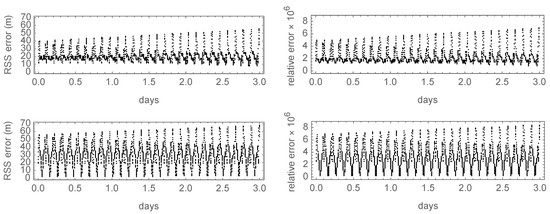
Figure 1.
Position errors of the test case: (top) noncanonical theory; (bottom) canonical theory.
Still with reference to Figure 1, we observe that the noncanonical solution seems slightly more accurate than its canonical counterpart for this particular example, with a root mean square error of m for the noncanonical theory as opposed to the m obtained in the canonical case. Nevertheless, both semianalytical solutions achieve the expected accuracy of a properly calibrated first-order solution along this time interval, with relative position errors , thus resulting in comparable performance regarding ephemeris (coordinate) computation.
Figure 2 displays the errors of the osculating elements obtained with the first-order theories, superimposed to linear fits to them. The only relevant differences between the two distinct theories are observed for the semimajor axis and for the eccentricity, whose errors in the three-day interval are presented in the first and second rows of Figure 2, respectively. For the former, the secular growth of the errors is of about 8 cm/day in both cases. However, the errors stemming from the noncanonical theory average just a few cm, whereas this average notably shifts to about 5 m in the case of the canonical solution—approximately two orders of magnitude higher. The behavior of the errors is analogous regarding the eccentricity, showing similar secular trends in both theories, of about /day. In this case, the increase in the average error obtained with the canonical solution is only about one order of magnitude larger than in the noncanonical case, yet clearly observable too. As with the coordinates, the amplitudes of the periodic errors affecting the orbital elements always dominate the picture, with the exception of the right ascension of the ascending node, where a secular trend of a few hundredths of an arc second per day is clearly apparent in the time histories obtained in both cases with periodic oscillations of about one tenth of as, as shown in the fourth row of Figure 2. Similar trends certainly exist in the time histories of the errors of and M, shown in the fifth and sixth rows of Figure 2, respectively, but they remain hidden in the figures due to the size of the periodic components of the errors of these two elements, whose amplitudes are about one order of magnitude larger than in the case of the right ascension of the ascending node. Finally, the behavior of the inclination errors is almost identical in the two theories, as shown in the graphics displayed in the third row of Figure 2, with very small secular trends whose rate falls below the mas/day whereas the amplitude of the periodic components of the errors is of just a few hundredths of as in both case. So, in spite of the comparable accuracy for ephemeris computation of the first-order solutions, the characteristic feature of the noncanonical theory of providing a better agreement with the true dynamics than the canonical case is clearly illustrated for the orbital elements with this example.
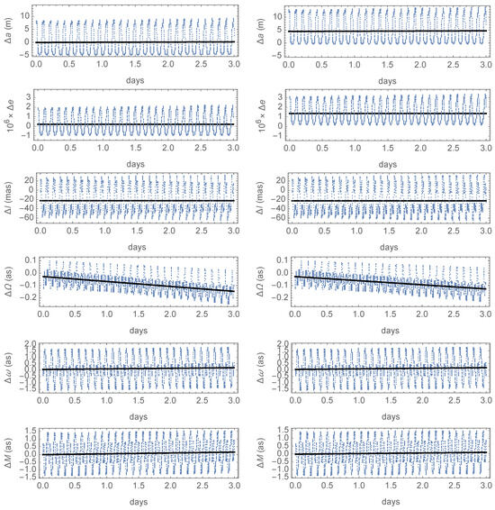
Figure 2.
Time histories of the errors of the orbital elements in the semianalytical integration of the test case: (left) noncanonical theory; (right) canonical theory.
5.2. Refinements of the Mean-to-Osculating Transformation
To obtain a better insight into the differences between the noncanonical and canonical approaches, we supplement both semianalytical solutions with the second-order terms of the respective mean-to-osculating transformation. As shown in Figure 3, now, the errors of the coordinates clearly disclose their respective secular trends, which are of about m/day in the noncanonical case, and only of 2 m per day for the canonical theory. Therefore, the semianalytic integrations clearly support the theoretical features discussed in the development of each theory. Namely, due to the existing terms in the mean variation of the Delaunay action that have been neglected by the truncation to the second order of , the secular errors grow at a slightly higher rate in the noncanonical case. Still, the periodic corrections are better captured by the noncanonical mean-to-osculating transformation, as indicated by the notably smaller amplitude of the periodic oscillations of the RSS position errors obtained with the improved solution.
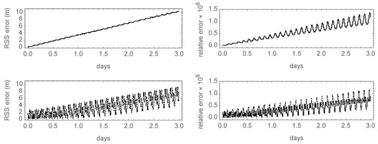
Figure 3.
Time histories of the position errors of the improved theories: (top) noncanonical case; (bottom) canonical case.
Regarding the errors of the osculating elements, the basic features shown by the first-order theories remain. However, the shifts from the zero average of the errors of the semimajor axis are now in the cm level in both cases, as clearly observed in Figure 4. While the errors in the semimajor axis are now of the same order of magnitude, a small bonus still goes to the side of the noncanonical case. More precisely, the average of the errors in the semimajor axis provided by the noncanonical theory falls slightly below the cm level, with insignificant periodic oscillations, compared to an average of about 1.5 cm in the canonical case, with periodic oscillations of much wider amplitude (see plots in the first row of Figure 4). The secular trend of the errors of the semimajor axis still exists but is negligible in both cases, falling below the mm/day level, yet with a lower slope on the side of the canonical theory.
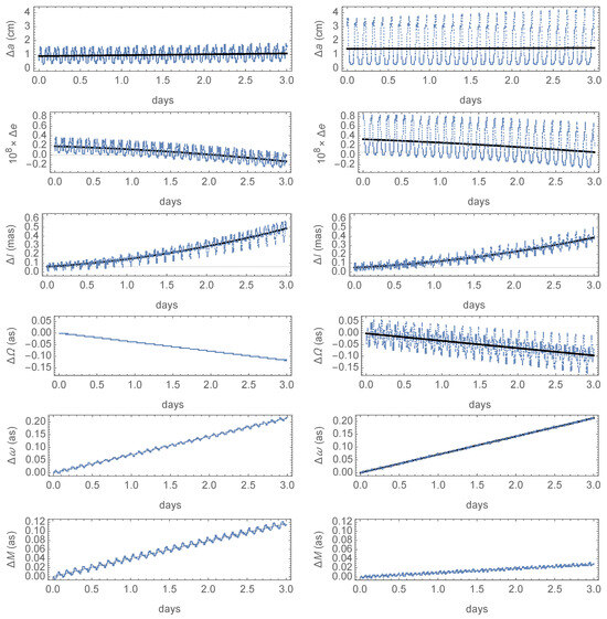
Figure 4.
Time histories of the errors of the orbital elements of the noncanonical (left) and canonical improved theories (right).
The much smaller oscillations of the errors due to the recovery of second-order, short-period effects now disclose a secular trend in the eccentricity errors. As observed in the plots of the second row of Figure 4, the secular trend shows a similar slope in both cases, but the periodic oscillations of the eccentricity errors remain clearly smaller on the side of the noncanonical theory. In fact, the fits superimposed to the time histories of the errors of the eccentricity have a small quadratic component in both cases.
On the other hand, the improvements in both perturbation theories disclose a quadratic growth of the inclination errors, but with a slower acceleration in the canonical case (refer to the third row of Figure 4). The short-period modulation of the time history of the inclination errors has now comparable amplitude when obtained with each solution, as it happened in the previous simulations, when using the first-order theories. The plots in the fourth row of Figure 4 show that the periodic components affecting the time histories of the errors in the propagation of the right ascension of the ascending node are mostly killed with the noncanonical theory, whereas their amplitudes remain below the arc second level in the canonical case; the secular, linear trend of the errors is similar in both cases, of just a few hundredths of as/day, yet with a slight advantage for the canonical perturbation solutions. The time history of the errors of the argument of the perigee presents almost identical behavior in both cases, with secular trends that grow at a rate smaller than one tenth of as/day, as observed in the plots of the fifth row of Figure 4). But this is not at all the case with the mean anomaly, where, as depicted in the plots of the lower row of Figure 4, a dramatic reduction in the slope of the time history of the errors is observed for the canonical solution when compared with the noncanonical case (about 10 mas/day vs. 39 mas/day, respectively).
In summary, the improvements in the mean-to-osculating transformation now bring both theories to a comparable level of accuracy as regards mimicking the average dynamics of the osculating elements, although the canonical solution generally shows a slightly worse performance than the noncanonical one regarding the amplitude of the periodic components of the errors. On the other hand, the effects of the truncation of the mean variation of the Delaunay action to second-order terms, which remained buried by the periodic components in the first-order solutions, are now clearly apparent in the time history of the errors of the mean anomaly. Indeed, while the truncation has little effect in the canonical case, where this mean variation vanishes by construction at any order of the perturbation approach, the errors due to the truncation of the noncanonical solution have a clear effect, which is translated directly into the corresponding faster growth of along-track errors.
That is, the exact separation of the short-period effects and the mean variations provides a better geometric description of the orbit, but at the expense of yielding larger along-track errors.
5.3. Additional Tuning
Because we have obtained the mean variations as well as the vectorial generating function of each different perturbation solution up to second-order terms, there is not too much difficulty in also computing the third-order terms of the mean variations.A whole other thing would be the computation of the third-order terms of the vector generators, in which task we could find serious difficulties in solving in closed form the indefinite integrals resulting from the Lie transforms procedure.While this challenging endeavor falls outside the scope of the current research, the much easier computation of the additional, third-order terms of the mean dynamics help us to confirm, and further illustrate, the different behavior of the tested solutions.
In spite of the fact that we lack the osculating-to-mean transformation of the Delaunay action that would allow us to achieve a proper initialization of the mean frequencies, the refinements of the mean variations with third-order terms yield clear improvements in the long-term effects of the errors. Yet, as expected, this kind of fine-tuning of the theories has little or no effect regarding the short-periodic oscillations of the errors. As illustrated in Figure 5, the errors obtained with both fine-tuned theories almost average to zero for all orbital elements, with the expected exception of the mean anomaly—whose linear growth has, nevertheless, halved in each case, thus further reducing the growth rate of the associated along-track errors. The time history of the errors of the semimajor axis remains almost the same as in the previous case at the precision of the graphics, and, therefore, corresponding plots are not displayed in Figure 5, whose direct comparison with Figure 4 makes the improvements evident otherwise. However, as expected from the previous theoretical discussions, the nonvanishing third-order terms of the mean variation of the Delaunay action in the case of the noncanonical solution radically improve the secular trend of the errors of the semimajor axis, whose rate now improves by more than one order of magnitude with respect to the previous simulation, falling to just a few hundredths of mm/day. On the contrary, the inclusion of third-order terms in the mean variations of the canonical solution does not result in appreciable improvements in the errors of the semimajor axis when compared to the previous propagation.
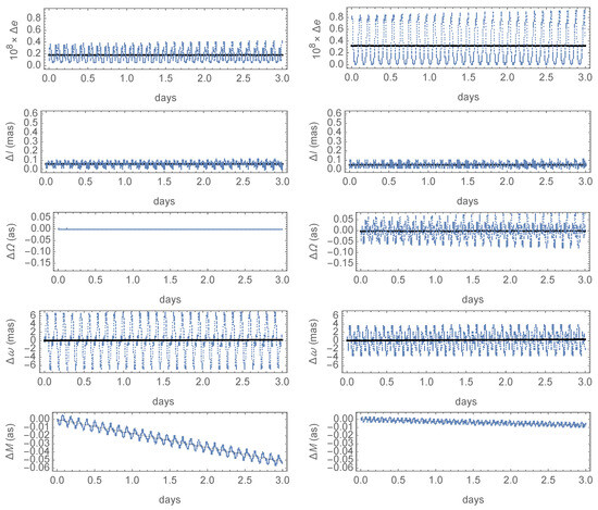
Figure 5.
Time histories of the errors of the orbital elements after the refinement of the noncanonical (left) and canonical theories (right) with third-order terms of the mean variations.
In reference to the other elements, the inclusion of the third-order terms in the mean variations means that the slope of the secular trend takes negligible values in the case of the eccentricity with both theories. More precisely, it falls below /day in the case of the noncanonical solution, yet it remains two orders of magnitude larger for the canonical case (graphics in the first row of Figure 5). For the inclination, the growth of the secular component of the errors is now of the order of as/day with both refined theories, with periodic components of the errors of analogous small amplitudes, as shown in the graphics displayed in the second row of Figure 5. The canonical solution shows a slightly better behavior for the right ascension of the ascending node regarding the secular trend, which is about mas/day compared to the mas/day of the noncanonical case. However, as shown in the third row of Figure 5, the latter shows periodic oscillations of the errors of comparable amplitude to those of the inclination errors, whereas the amplitude of the periodic components of the former is two orders of magnitude larger. The secular trend in the time history of the errors of the argument of the perigee is reduced in both cases from the tenths of as obtained in the previous simulations to an analogous fraction of mas in the current case (graphics in the fourth row of Figure 5). Finally, the graphics in the lower plots of Figure 5 show the already mentioned advantage of the canonical solution regarding the errors associated to the mean anomaly, with a small secular rate of about mas/day contrasting with the mas/day of the noncanonical solution.
For additional insight, the corresponding improvements of the position errors obtained with the supplementary, long-period, third-order terms of each theory are depicted in Figure 6, where a linear fit to the errors is superimposed to their time histories to better illustrate their secular growth (black, solid lines in the graphics of the left column of Figure 6). This kind of representation confirms the advantage of the canonical theory regarding the growth of in-track errors, showing a secular trend of the RSS errors of about 80 cm/day in the noncanonical case, displayed in the upper plots of Figure 6, as opposed to the only 5 cm/day of the canonical case presented in the lower plots of the same figure. However, the contribution of the periodic components of the RSS errors makes the accuracy of both theories comparable in this 3-day interval, resulting in a root mean square error of m in the noncanonical case, against m in the canonical case, which, while smaller, remains clearly comparable.
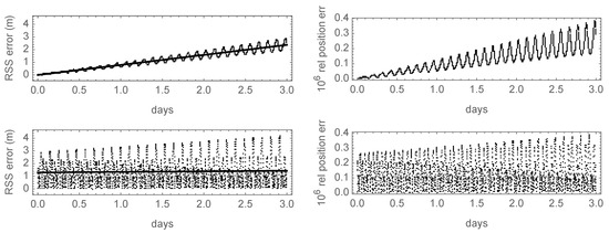
Figure 6.
Position errors of the improved theories with third-order long-period terms: (top) noncanonical case; (bottom) canonical case.
Nevertheless, the higher growth rate of the secular errors of the noncanonical case soon or later will dominate the picture. As shown in the left plot of Figure 7, this is exactly the case, and the position errors stemming from the noncanonical solution clearly overcome those of the canonical case after the first 10 days. Still, including third-order terms is not common in operational semianalytical theories due to the many different perturbations that in fact contribute second-order terms, and are not included in the current research. As further illustrated with the right plot of Figure 7, when truncated to second-order effects, both semianalytical theories may also provide comparable position errors in the case of long-term propagations.
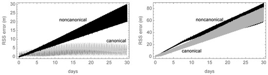
Figure 7.
Position errors of the improved theories with third-order long-period terms (left plot) and with only second-order terms (right plot).
6. Conclusions
For the main problem of artificial satellite theory, the second-order terms of the purely periodic, noncanonical transformation yielding the exact separation of long- and short-period effects were computed in closed form for the first time. The noncanonical transformation was computed in Delaunay canonical variables, which are usually criticized for their shortcomings in the treatment of low-eccentricity orbits. Still, because the noncanonical solution was computed with the method of Lie transforms, the reformulation of the semianalytical solution in any desired set of nonsingular variables in no way requires to recompute the perturbation theory from scratch. On the contrary, the nonsingular perturbation solution can be derived directly from the already computed vectorial generator in Delaunay variables under some additional constraints. Such reformulation is under development and will be reported elsewhere.
On the other hand, the use of Delaunay canonical variables helped us to check the canonical character of a mean-to-osculating transformation based on the choice of a vectorial generator whose components are purely periodic in the mean anomaly. The comparison of the results obtained when the two different approaches were applied the main problem confirmed previous conjectures based on simplified, toy models. To wit, the noncanonical perturbation solution resulted in a better geometric description of the integrated orbit, and remained closer to the mean elements dynamics due to a more suitable handling of its short-period components. However, this appealing advantage was at the expense of a worse realization of the mean variation of the semimajor axes. Because of that, the errors in the semianalytical integration of the mean anomaly with the noncanonical solution grew at a faster rate than in the canonical case, with the consequent increase in the along-track errors. This later fact may make preferable the canonical approach for long-term ephemeris propagation—which, incidentally, does not need to be computed by Hamiltonian methods, as it is already known and we further demonstrated it with the results discussed in the paper.
Funding
This research has received funding from the Spanish State Research Agency and the European Regional Development Fund (Project PID2021-123219OB-I00, AEI/ERDF, EU).
Data Availability Statement
Data is contained within the article.
Conflicts of Interest
The author declares no conflict of interest.
Appendix A. Integration of Some Functions of the Equation of the Center
As soon as we begin the computation of second-order terms of the generating function of the Lie transforms solution, we confront the closed-form integration of integrals involving the equation of the center , of the type
where . Noting that , and using integration by parts, for , we obtain
where is, in turn, integrated by parts, to give
a result that was first reported in [34]. Hence, Equation (A1) turns into
The rules for the integration of in the mean anomaly are detailed in [20], whereas the indefinite integration of in the mean anomaly corresponds to case (v) of [22].
Using the previous result and on account of the fundamental theorem of calculus, we readily obtain
where both quadratures on the right side of the equation are readily integrated following the rules in [18] regarding the first quadrature, and in [21] for the second one.
References
- Hansen, P.A. Expansions of the product of a power of the radius vector with the sinus or cosinus of a multiple of the true anomaly in terms of series containing the sinuses or cosinuses of the multiples of the true, eccentric or mean anomaly. Abh. Der Königlich Sächsischen Ges. Der Wiss. 1855, 2, 183–281. [Google Scholar]
- Delaunay, C.E. La Théorie du Mouvement de la Lune, Premier Volume; Mémoires de l’Academie des Sciences de l’Institut Impérial de France; Mallet-Bachellier: Paris, France, 1860; Volume 28. [Google Scholar]
- Tisserand, F. Traité de Mécanique Céleste. Tome I: Perturbations des Planètes D’aprés la Méthode de la Variation des Constantes Arbitraries; Gauthier-Villars et fils: Paris, France, 1889. [Google Scholar]
- Zeipel, H.V. Research on the Motion of Minor Planets; NASA TT F-9445; NASA Translation of: Recherches sur le Mouvement des Petites Planètes, Arkiv för Matematik, Astronomi och Fysik, Volume 11, 1916, Volume 12, 1917, Volume 13, 1918; National Aeronautics and Space Administration: Washington, DC, USA, 1965. [Google Scholar]
- Garfinkel, B. The orbit of a satellite of an oblate planet. Astron. J. 1959, 64, 353–367. [Google Scholar] [CrossRef]
- Brouwer, D. Solution of the problem of artificial satellite theory without drag. Astron. J. 1959, 64, 378–397. [Google Scholar] [CrossRef]
- Kozai, Y. The motion of a close earth satellite. Astron. J. 1959, 64, 367–377. [Google Scholar] [CrossRef]
- Vallado, D.A. Fundamentals of Astrodynamics and Applications, 4th ed.; Microcosm: Hawthorne, CA, USA, 2013. [Google Scholar]
- Brouwer, D.; Clemence, G.M. Methods of Celestial Mechanics; Academic Press: New York, NY, USA; London, UK, 1961. [Google Scholar]
- Giacaglia, G.E.O. A note on Hansen’s coefficients in satellite theory. Celest. Mech. 1976, 14, 515–523. [Google Scholar] [CrossRef]
- Deprit, A.; Rom, A. The Main Problem of Artificial Satellite Theory for Small and Moderate Eccentricities. Celest. Mech. 1970, 2, 166–206. [Google Scholar] [CrossRef]
- Kinoshita, H. Third-Order Solution of an Artificial-Satellite Theory. SAO Spec. Rep. 1977, 379, 1–106. [Google Scholar]
- Kozai, Y. Second-order solution of artificial satellite theory without air drag. Astron. J. 1962, 67, 446–461. [Google Scholar] [CrossRef]
- Métris, G.; Exertier, P. Semi-analytical theory of the mean orbital motion. Astron. Astrophys. 1995, 294, 278–286. [Google Scholar]
- Morrison, J.A. Generalized Method of Averaging and the Von Zeipel Method. In Methods in Astrodynamics and Celestial Mechanics; Duncombe, R.L., Szebehely, V.G., Eds.; Progress in Astronautics and Rocketry; Elsevier: Amsterdam, The Netherlands, 1966; Volume 17, pp. 117–138. [Google Scholar] [CrossRef]
- Lara, M.; San-Juan, J.F.; Folcik, Z.J.; Cefola, P. Deep Resonant GPS-Dynamics Due to the Geopotential. J. Astronaut. Sci. 2011, 58, 661–676. [Google Scholar] [CrossRef]
- Lara, M.; San-Juan, J.F.; López-Ochoa, L.M. Proper Averaging Via Parallax Elimination (AAS 13-722). In Proceedings of the Astrodynamics 2013; Broschart, S.B., Turner, J.D., Howell, K.C., Hoots, F.R., Eds.; Advances in the Astronautical Sciences; American Astronautical Society: San Diego, CA, USA, 2014; Volume 150, pp. 315–331. [Google Scholar]
- Kozai, Y. Mean values of cosine functions in elliptic motion. Astron. J. 1962, 67, 311–312. [Google Scholar] [CrossRef]
- Deprit, A.; Ferrer, S. Note on Cid’s Radial Intermediary and the Method of Averaging. Celest. Mech. 1987, 40, 335–343. [Google Scholar] [CrossRef]
- Kelly, T.S. A note on first-order normalizations of perturbed Keplerian systems. Celest. Mech. Dyn. Astron. 1989, 46, 19–25. [Google Scholar] [CrossRef]
- Metris, G. Mean values of particular functions in the elliptic motion. Celest. Mech. Dyn. Astron. 1991, 52, 79–84. [Google Scholar] [CrossRef]
- Ahmed, M.K.M. On the normalization of perturbed Keplerian systems. Astron. J. 1994, 107, 1900–1903. [Google Scholar] [CrossRef]
- Ferraz-Mello, S. Do Average Hamiltonians Exist? Celest. Mech. Dyn. Astron. 1999, 73, 243–248. [Google Scholar] [CrossRef]
- McClain, W.D. A Recursively Formulated First-Order Semianalytic Artificial Satellite Theory Based on the Generalized Method of Averaging, Volume 1: The Generalized Method of Averaging Applied to the Artificial Satellite Problem, 2nd ed.; NASA CR-156782; NASA: Greenbelt, ML, USA, 1977. [Google Scholar]
- Liu, J.J.F.; Alford, R.L. Semianalytic Theory for a Close-Earth Artificial Satellite. J. Guid. Control Dyn. 1981, 4, 576. [Google Scholar] [CrossRef]
- Kaufman, B. First order semianalytic satellite theory with recovery of the short period terms due to third body and zonal perturbations. Acta Astronaut. 1981, 8, 611–623. [Google Scholar] [CrossRef]
- Coffey, S.L.; Neal, H.L.; Segerman, A.M.; Travisano, J.J. An Analytic Orbit Propagation Program for Satellite Catalog Maintenance. In Proceedings of the AAS/AIAA Astrodynamics Conference 1995; Alfriend, K.T., Ross, I.M., Misra, A.K., Peters, C.F., Eds.; Advances in the Astronautical Sciences; American Astronautical Society: San Diego, CA, USA, 1996; Volume 90, pp. 1869–1892. [Google Scholar]
- Lara, M.; San-Juan, J.F.; Hautesserres, D. HEOSAT: A mean elements orbit propagator program for highly elliptical orbits. CEAS Space J. 2018, 10, 3–23. [Google Scholar] [CrossRef]
- Lara, M. On mean elements in artificial-satellite theory. Celest. Mech. Dyn. Astron. 2023, 135, 43. [Google Scholar] [CrossRef]
- Lara, M. Exact separation of long- and short-period effects in the computation of mean elements of artificial satellite theory (IAC-23,C1,8,5). In Proceedings of the 74th International Astronautical Congress (IAC), Baku, Azerbaijan, 2–6 October 2023; International Astronautical Federation (IAF): Paris, France, 2023; pp. 1–10. [Google Scholar]
- Jefferys, W.H. Automated, Closed Form Integration of Formulas in Elliptic Motion. Celest. Mech. 1971, 3, 390–394. [Google Scholar] [CrossRef]
- Deprit, A. Delaunay normalisations. Celest. Mech. 1982, 26, 9–21. [Google Scholar] [CrossRef]
- Healy, L.M. The Main Problem in Satellite Theory Revisited. Celest. Mech. Dyn. Astron. 2000, 76, 79–120. [Google Scholar] [CrossRef]
- Lara, M. Brouwer’s satellite solution redux. Celest. Mech. Dyn. Astron. 2021, 133, 1–20. [Google Scholar] [CrossRef]
- Wang, Y.; Sun, X.; He, L.; Liu, S.; He, W. An accurate and efficient second-order J2 model for the Draper semianalytic satellite theory. Acta Astronaut. 2024, 225, 169–185. [Google Scholar] [CrossRef]
- Hoots, F.R.; Roehrich, R.L. Models for Propagation of the NORAD Element Sets; Project SPACETRACK, Rept. 3; U.S. Air Force Aerospace Defense Command: Colorado Springs, CO, USA, 1980. [Google Scholar]
- Coffey, S.; Alfriend, K.T. An analytical orbit prediction program generator. J. Guid. Control Dyn. 1984, 7, 575–581. [Google Scholar] [CrossRef]
- Hoots, F.R.; Schumacher, P.W., Jr.; Glover, R.A. History of Analytical Orbit Modeling in the U. S. Space Surveillance System. J. Guid. Control. Dyn. 2004, 27, 174–185. [Google Scholar] [CrossRef]
- Vallado, D.A.; Crawford, P.; Hujsak, R.; Kelso, T.S. Revisiting Spacetrack Report #3 (AIAA 2006-6753). In Proceedings of the AIAA/AAS Astrodynamics Specialist Conference and Exhibit, Guidance, Navigation, and Control and Co-Located Conferences, Keystone, CO, USA, 21–24 August 2006; pp. 1–88. [Google Scholar] [CrossRef]
- Deprit, A. Canonical transformations depending on a small parameter. Celest. Mech. 1969, 1, 12–30. [Google Scholar] [CrossRef]
- Kamel, A.A. Perturbation Method in the Theory of Nonlinear Oscillations. Celest. Mech. 1970, 3, 90–106. [Google Scholar] [CrossRef]
- Henrard, J. On a perturbation theory using Lie transforms. Celest. Mech. 1970, 3, 107–120. [Google Scholar] [CrossRef]
- Lyddane, R.H. Small eccentricities or inclinations in the Brouwer theory of the artificial satellite. Astron. J. 1963, 68, 555–558. [Google Scholar] [CrossRef]
- Lara, M. Earth satellite dynamics by Picard iterations. arXiv 2022, arXiv:2205.04310. [Google Scholar]
- Arsenault, J.L.; Ford, K.C.; Koskela, P.E. Orbit determination using analytic partial derivatives of perturbed motion. AIAA J. 1970, 8, 4–12. [Google Scholar] [CrossRef]
- Hintz, G. Survey of Orbit Element Sets. J. Guid. Control. Dyn. 2008, 31, 785–790. [Google Scholar] [CrossRef]
- Danby, J.M.A. Motion of a Satellite of a Very Oblate Planet. Astron. J. 1968, 73, 1031–1038. [Google Scholar] [CrossRef]
- Broucke, R.A. Numerical integration of periodic orbits in the main problem of artificial satellite theory. Celest. Mech. Dyn. Astron. 1994, 58, 99–123. [Google Scholar] [CrossRef]
- Lara, M. Hamiltonian Perturbation Solutions for Spacecraft Orbit Prediction. The Method of Lie Transforms, 1st ed.; De Gruyter Studies in Mathematical Physics; De Gruyter: Berlin, Germany; Boston, FL, USA, 2021; Volume 54, p. xv, 377. [Google Scholar] [CrossRef]
- Irigoyen, M.; Simó, C. Non integrability of the J2 problem. Celest. Mech. Dyn. Astron. 1993, 55, 281–287. [Google Scholar] [CrossRef]
- Celletti, A.; Negrini, P. Non-integrability of the problem of motion around an oblate planet. Celest. Mech. Dyn. Astron. 1995, 61, 253–260. [Google Scholar] [CrossRef]
- Simó, C. Measuring the lack of integrability of the J2 problem for Earth’s satellites. In Predictability, Stability, and Chaos in N-Body Dynamical Systems; NATO Advanced Study Institute (ASI) Series B; Springer: New York, NY, USA, 1991; Volume 272, pp. 305–309. [Google Scholar]
- Steichen, D.; Giorgilli, A. Long Time Stability for the Main Problem of Artificial Satellites. Celest. Mech. Dyn. Astron. 1997, 69, 317–330. [Google Scholar] [CrossRef]
- Lara, M. Solution to the main problem of the artificial satellite by reverse normalization. Nonlinear Dyn. 2020, 101, 1501–1524. [Google Scholar] [CrossRef]
- Scheifele, G.; Graf, O. Analytical satellite theories based on a new set of canonical elements. In Proceedings of the Mechanics and Control of Flight Conference, Reston, VI, USA, 5–9 August 1974; pp. 1–20. [Google Scholar] [CrossRef]
- Deprit, A. The Main Problem in the Theory of Artificial Satellites to Order Four. J. Guid. Control Dyn. 1981, 4, 201–206. [Google Scholar] [CrossRef]
- Coffey, S.L.; Deprit, A. Third-Order Solution to the Main Problem in Satellite Theory. J. Guid. Control Dyn. 1982, 5, 366–371. [Google Scholar] [CrossRef]
- Wnuk, E. Recent progress in analytical orbit theories. Adv. Space Res. 1999, 23, 677–687. [Google Scholar] [CrossRef]
- Palacián, J.F. Dynamics of a satellite orbiting a planet with an inhomogeneous gravitational field. Celest. Mech. Dyn. Astron. 2007, 98, 219–249. [Google Scholar] [CrossRef]
- Lara, M. Note on the analytical integration of circumterrestrial orbits. Adv. Space Res. 2022, 69, 4169–4178. [Google Scholar] [CrossRef]
- Lara, M.; Fantino, E.; Susanto, H.; Flores, R. Higher-order composition of short- and long-period effects for satellite analytical ephemeris computation. Commun. Nonlinear Sci. Numer. Simul. 2024, 137, 108023. [Google Scholar] [CrossRef]
- Lara, M. Improving efficiency of analytic orbit propagation (IAC-21,C1,7,2,x65390). In Proceedings of the 72nd International Astronautical Congress (IAC), Dubai, United Arab Emirates, 25–29 October 2021; International Astronautical Federation (IAF): Paris, France, 2021; pp. 1–10. [Google Scholar]
- Poincaré, H. Les Méthodes Nouvelles de la Mécanique Céleste. Tome 2. Les Méthodes de MM. Newcomb, Gylden, Lindstedt et Bohlin; Gauthier-Villars et fils: Paris, France, 1893. [Google Scholar]
- Hori, G.i. Theory of General Perturbation with Unspecified Canonical Variables. Publ. Astron. Soc. Jpn. 1966, 18, 287–296. [Google Scholar]
- Nayfeh, A.H. Perturbation Methods; Wiley-VCH Verlag GmbH & Co. KGaA: Weinheim, Germany, 2004. [Google Scholar]
- Murdock, J.A. Perturbations: Theory and Methods; Classics in Applied Mathematics; SIAM–Society for Industrial and Applied Mathematics: Philadelphia, PA, USA, 1999; Volume 27, p. 509. [Google Scholar] [CrossRef]
- Danielson, D.A.; Sagovac, C.P.; Neta, B.; Early, L.W. Semianalytic Satellite Theory; Technical Report NPS-MA-95-002; Naval Postgraduate School: Monterey, CA, USA, 1995. [Google Scholar]
- Henrard, J. Analytical drag theory of an artificial satellite with small eccentricity. In Proceedings of the Space Dynamics and Celestial Mechanics, Delhi, India, 14–16 November 1985; Bhatnagar, K., Ed.; International Workshop: Dordrecht, The Netherlands, 1986. Astrophysics and Space Science Library. Volume 127, pp. 261–272. [Google Scholar] [CrossRef]
- Barrio, R.; Palacián, J. High-order averaging of eccentric artificial satellites perturbed by the Earth’s potential and air-drag terms. Proc. R. Soc. Lond. Ser. A 2003, 459, 1517–1534. [Google Scholar] [CrossRef]
- Breakwell, J.V.; Vagners, J. On Error Bounds and Initialization in Satellite Orbit Theories. Celest. Mech. 1970, 2, 253–264. [Google Scholar] [CrossRef]
- Armellin, R.; San-Juan, J.F.; Lara, M. End-of-life disposal of high elliptical orbit missions: The case of INTEGRAL. Adv. Space Res. 2015, 56, 479–493. [Google Scholar] [CrossRef]
- Cain, B.J. Determination of mean elements for Brouwer’s satellite theory. Astron. J. 1962, 67, 391–392. [Google Scholar] [CrossRef]
- Walter, H.G. Conversion of osculating orbital elements into mean elements. Astron. J. 1967, 72, 994–997. [Google Scholar] [CrossRef]
- Eckstein, M.C.; Hechler, F. A Reliable Derivation of the Perturbations due to Any Zonal and Tesseral Harmonics of the Geopotential for Nearly-Circular Satellite Orbits; Scientific Report ESRO SR-13; European Space Research Organisation: Darmstadt, Germany, 1970. [Google Scholar]
- Gaias, G.; Colombo, C.; Lara, M. Analytical Framework for Precise Relative Motion in Low Earth Orbits. J. Guid. Control Dyn. 2020, 43, 915–927. [Google Scholar] [CrossRef]
- Lyddane, R.H.; Cohen, C.J. Numerical comparison between Brouwer’s theory and solution by Cowell’s method for the orbit of an artificial satellite. Astron. J. 1962, 67, 176–177. [Google Scholar] [CrossRef]
- Bonavito, N.L.; Watson, S.; Walden, H. An Accuracy and Speed Comparison of the Vinti and Brouwer Orbit Prediction Methods; Technical Report NASA TN D-5203; Goddard Space Flight Center: Greenbelt, ML, USA, 1969. [Google Scholar]
- Stiefel, E.L.; Scheifele, G. Linear and Regular Celestial Mechanics, 1st ed.; Grundlehren der mathematischen Wissenschaften; Springer: Berlin/Heidelberg, Germany, 1971; Volume 174, p. x, 306. [Google Scholar]
- Battin, R.H. An Introduction to the Mathematics and Methods of Astrodynamics; American Institute of Aeronautics and Astronautics, Inc.: Reston, VG, USA, 1999. [Google Scholar]
- Roy, A.E. Orbital Motion, 4th ed.; Institute of Physics Publishing: Bristol, UK, 2005; p. XVIII + 526. [Google Scholar]
Disclaimer/Publisher’s Note: The statements, opinions and data contained in all publications are solely those of the individual author(s) and contributor(s) and not of MDPI and/or the editor(s). MDPI and/or the editor(s) disclaim responsibility for any injury to people or property resulting from any ideas, methods, instructions or products referred to in the content. |
© 2025 by the author. Licensee MDPI, Basel, Switzerland. This article is an open access article distributed under the terms and conditions of the Creative Commons Attribution (CC BY) license (https://creativecommons.org/licenses/by/4.0/).