Convective Flux Analysis on the Instability of One-Dimensional Detonation

Abstract

One-dimensional numerical simulations using the Euler equations and irreversible one-step Arrhenius kinetics are conducted to study the instability mechanism of a one-dimensional gaseous detonation. By increasing the activation energy, this study identifies the characteristics of stable detonation, periodic detonation, pulsating detonation, and detonation quenching. The key difference between this study and previous research is that it is the first quantitative analysis of convective flux, kinetic energy flux, and chemical reaction heat flux. These three fluxes undergo intensive change on the detonation front and the flow field at each time step depends on the algebraic summation of them. The mechanisms of detonation instability, detonation reignition, and the detonation quenching process can be revealed quantitatively by analyzing these fluxes. The detonation instability is the intrinsic property of the reactive Euler system.

1. Introduction

Detonation is a supersonic combustion wave in which the reactants are ignited by the shock wave and the energy released from the chemical reaction is coupled with the shock wave to sustain its propagation [1]. Two important theories of steady detonation, the Chapman–Jouguet (C-J) theory and the Zeldovich–von Neumann–Doring (ZND) theory, have been frequently used in detonation studies. However, detonation is inherently unstable and understanding detonation instability remains a key challenge in detonation theory.

One method of investigating detonation instability is linear stability analysis, which imposes small perturbations on the steady solution to determine whether the amplitude of the perturbations grows or not. The assumption of small perturbations allows linearization and integration of the equations, enabling the identification of unstable modes. The linear stability analysis of detonation stability was first developed by Erpenbeck to investigate the stability behavior of an idealized detonation [2,3,4]. Using the Laplace transform approach discussed in his work, the overall linear stability of a detonation was first demonstrated mathematically by analyzing the governing equations with perturbation involved in the problem.

Lee and Stewart developed a normal mode approach to address the same problem by using a numerical shooting algorithm under the acoustic boundary condition at the end of the reaction [5]. Sharpe derived a similar approach based on the normal mode analysis and obtained an asymptotic solution for the ordinary differential equations for the linear perturbations [6]. Short conducted similar studies [7,8]. A detailed review of the normal mode stability formulation was given by Gorchkov et al. [9]. Uy et al. conducted linear stability analysis of one-dimensional detonation coupled with vibrational relaxation and the Landau–Teller model was applied to specify the vibrational relaxation [10]. Xu et al. studied the pulsating behavior and stability parameters of one-dimensional non-ideal detonations [11]. Non-ideal detonations were modeled with two-step consecutive irreversible reactions to represent endothermic effects.

As with most hydrodynamic stability analyses, the dispersion relation is complex and cannot be expressed analytically, making it difficult to elucidate the physical basis of the stability mechanism. It should be noted that linear stability analyses are valid only for the initial growth of the perturbations and cannot describe the results far from the stability limits or the final nonlinear unstable structure of the detonation [1]. Thus, it is rather difficult to obtain physical insight into the stability mechanisms. Furthermore, linear stability analyses do not reveal the gas-dynamic mechanisms behind the generation of the instability.

Another method is direct numerical simulation of computational fluid dynamics (CFD), which employs time-dependent, nonlinear, compressible, and reactive Euler equations. Unlike the linear stability analysis, the direct numerical simulations have the advantage that the full nonlinearity of the problem is retained. A series of numerical studies were conducted by Sharp et al. using a two-step chain-branching reaction model [12,13,14], Short et al. using a three-step chain-branching reaction model [15,16] and Hwang et al. [17]. Ng et al. conducted numerical simulations to study the nonlinear dynamics and chaos analysis of one-dimensional pulsating detonations [18,19]. The Euler equations with overall one-step Arrhenius kinetics were used. One notable characteristic is that varying the activation energy control parameter can cause the pulsation pattern to transition from periodic to highly irregular, or chaotic, structures.

Kasimov and Stewart proposed an improved numerical simulation method that integrates the governing equations in a shock-attached frame with a nonreflecting boundary condition [20]. Henrick et al. numerically simulated the pulsating one-dimensional detonations with fifth-order accuracy [21]. A novel, highly accurate numerical scheme based on shock-fitting coupled with a fifth-order WENO scheme was applied to the classical unsteady detonation problem to generate solutions with unprecedented accuracy. As the activation energy is increased, a series of period-doubling events are predicted and the system undergoes a transition to chaos. The bifurcation points are seen to converge at a rate of the Feigenbaum constant, which is consistent with the theory of nonlinear dynamics. Powers authored a detailed review of multiscale modeling of detonation [22].

Choi et al. [23] systematically discussed the effect of several numerical issues, including the effect of grid size, time step, computational domain, and boundary conditions, on the simulation of detonation cellular structure with variable stability regimes ranging from weakly to highly unstable detonations. In higher dimensions, the effect of chaos may play a prominent role in detonation instability [24]. The two-dimensional detonation cellular structure is fundamentally shaped by pulsating instability. The detonation in free space was numerically simulated to understand the evolution of the one-dimensional pulsating instability and two-dimensional cellular structure [25,26]. It is found that the pulsation occurs in three stages: (1) rapid decay of the overdrive, (2) transition to the Chapman–Jouguet state accompanied by weak pulsations, and (3) development of strong pulsations. A chemical explosive mode analysis further confirmed the highly autoignition nature of the mixture in the induction zone between reaction front and shock front, where thermal diffusion plays a negligible role [27].

Although the bifurcation diagram was constructed from previous computational results, the theoretical explanation for how the instability pattern transitions to chaos remains unclear. The mechanisms of detonation quenching and the thermodynamics of deflagration wave were discussed by analyzing the convective flux and heat release flux in one-dimensional numerical simulation [28]. It was first revealed that the convective flux plays an important role in detonation instability. This study is an in-depth extension of the previous work, which discusses the mechanism of detonation instability systematically.

2. Governing Equations and Numerical Methods

The governing equations are the one-dimensional Euler equations incorporating overall one-step irreversible Arrhenius chemical reaction kinetics. Viscosity, diffusion, and heat conduction are neglected. The conservation form of the mass, momentum, energy, and species equations is presented here.

$${\displaystyle \frac{\partial U}{\partial t}}+{\displaystyle \frac{\partial F}{\partial x}}=S$$

(1)

where the conservation variable $U$, the convective flux $F$ and the reactive source term $S$ are, respectively,

$$U=\left(\begin{array}{c}\rho \\ \rho u\\ \rho e\\ \rho Z\end{array}\right) F=\left(\begin{array}{c}\rho u\\ \rho u^2+p\\ (\rho e+p)u\\ \rho uZ\end{array}\right) S=\left(\begin{array}{c}0\\ 0\\ 0\\ \dot{\omega }\end{array}\right)$$

(2)

$$e={\displaystyle \frac{p}{\left(\gamma -1\right)\rho }}+{\displaystyle \frac{1}{2}}{u}^2+Zq$$

(3)

$$p=\rho RT$$

(4)

$$\dot{\omega }=-K\rho Z\exp \left(-{\displaystyle \frac{C{E}_{\mathrm{a}}\left(\gamma -1\right)}{RT}}\right)$$

(5)

$$\gamma (Z)={\displaystyle \frac{{\gamma }_1{R}_{1}Z/({\gamma }_1-1)+{\gamma }_2{R}_2(1-Z)/({\gamma }_2-1)}{R_{1}Z/({\gamma }_1-1)+R_2(1-Z)/({\gamma }_2-1)}}$$

(6)

$$R(Z)=R_{1}Z+R_2(1-Z)$$

(7)

In the above equations, $\rho$, $p$, $u$, $e$, $q$, $R$, $\gamma$ and $Z$ are density, pressure, velocity, specific total energy, specific heat release per unit mass of reactant, gas constant, specific heat ratio and the chemical reaction progress parameter, respectively. $\dot{\omega }$ is the mass production rate of combustion products, $K$ is the pre-exponential factor, $T$ is the temperature in Kelvin K, and $E_a$ is the activation energy, respectively. The parameter $C$ in Equation (5) is a controlling parameter used to change the activation energy in different numerical cases. The subscripts 1 and 2 in Equations (6) and (7) represent the reactants and products, respectively.

According to Equations (8)–(11), the pressure gain Δp at one time step is determined by three terms: the convective flux, the kinetic energy term and the heat release term. To facilitate numerical analysis, we define the convective flux (Γ), the enthalpy flux (F_E), the kinetic energy term (ΔK), and the chemical reaction heat release flux (ΔQ) at each time step. In the numerical simulations, at each time step, Γ > 0 on the detonation front refers to the shock wave and Γ < 0 on the detonation front refers to the rarefaction wave.

$$U^{n+1}=U^n-{\displaystyle \frac{\partial F^n}{\partial x}}\mathrm{\Delta }t+S^n\mathrm{\Delta }t$$

(8)

$$\mathrm{\Delta }(\rho e)={\left(\rho e\right)}^{n+1}-{\left(\rho e\right)}^n=-{\displaystyle \frac{\partial \left(\rho e+p\right)u}{\partial x}}\mathrm{\Delta }t$$

(9)

$$\rho e={\displaystyle \frac{p}{\left(\gamma -1\right)}}+{\displaystyle \frac{1}{2}}\rho u^2+\rho Zq$$

(10)

$$\mathrm{\Delta }p=p^{n+1}-p^n=\left(\mathrm{\Delta }(\rho e)-\mathrm{\Delta }\left({\displaystyle \frac{1}{2}}\rho u^2\right)-\mathrm{\Delta }\left(\rho Zq\right)\right)\left(\gamma -1\right)$$

(11)

$$F_E=\left(\rho e+p\right)u$$

(12)

$$\mathrm{\Gamma }=\mathrm{\Delta }(\rho e)=-{\displaystyle \frac{\partial \left(\rho e+p\right)u}{\partial x}}\mathrm{\Delta }t$$

(13)

$$\mathrm{\Delta }Q=-\mathrm{\Delta }\left(\rho qZ\right)={\rho }^n{Z}^{\mathrm{n}}q-{\rho }^{n+1}{Z}^{\mathrm{n}+1}q$$

(14)

$$\mathrm{\Delta }K=-\mathrm{\Delta }\left({\displaystyle \frac{1}{2}}\rho u^2\right)={\displaystyle \frac{1}{2}}{\rho }^n{\left(u^n\right)}^2-{\displaystyle \frac{1}{2}}{\rho }^{n+1}{\left(u^{n+1}\right)}^2$$

(15)

$$\mathrm{\Delta }p=\left(\mathrm{\Gamma }+\mathrm{\Delta }K+\mathrm{\Delta }Q\right)\left(\gamma -1\right)$$

(16)

This methodology can be easily extended to multidimensional detonation. For instance, the convective flux and kinetic energy term of a three-dimensional laminar detonation with Navier–Stokes equations become

$$\mathrm{\Gamma }=\mathrm{\Delta }(\rho e)=-{\displaystyle \frac{\partial \left(\rho e+p\right)u_i}{\partial x_i}}\mathrm{\Delta }t+{\displaystyle \frac{\partial }{\partial x_i}}\left[\alpha {\displaystyle \frac{\partial T}{\partial x_i}}+u_j{\tau }_{ij}\right]\mathrm{\Delta }t$$

(17)

$${\tau }_{ij}=\mu \left({\displaystyle \frac{\partial u_i}{\partial x_j}}+{\displaystyle \frac{\partial u_j}{\partial x_i}}-{\displaystyle \frac{2}{3}}{\delta }_{ij}{\displaystyle \frac{\partial u_k}{\partial x_k}}\right)$$

(18)

$$\mathrm{\Delta }K=-\mathrm{\Delta }\left({\displaystyle \frac{1}{2}}\rho {u_i}^2\right)$$

(19)

In the above equations, $u_i$ represents the velocity components, $\alpha$ is the laminar thermal conductivity, ${\tau }_{ij}$ is the viscous stress tensor, $\mu$ is the dynamic viscosity, and ${\delta }_{ij}$ is the Kronecker symbol, respectively.

According to Equation (9), to maintain detonation propagation, the gas on the detonation front must maintain a higher enthalpy value. This means that the gas on the detonation front should obtain higher pressure gain Δp through chemical heat release at each time step. The value of kinetic energy term ΔK in Equation (16) is negative. Therefore, according to Equation (16), the positive summit of convective flux Γ and the summit of heat release ΔQ should be at the same grid point at every time step in order to obtain higher enthalpy. In other words, the flame front should be tightly coupled with the shock wave. However, the position of heat release is controlled by the Arrhenius law. If the flame is decoupled from the shock wave front under higher activation energy, the peaks of heat release and shock wave are not at the same grid point, and the pressure gain by heat release becomes smaller. The physics of these fluxes at one grid point and one time step are summarized briefly in Table 1.

Table 1. The physics of three fluxes.

No.	Modes	Physics of Flow Field
1	Γ > 0, ΔQ > 0, ΔK < 0	Total energy per unit volume is increased; heat is released; both are converted into internal energy and kinetic energy; C-J detonation.
2	Γ > 0, ΔQ = 0, ΔK < 0	Total energy per unit volume is increased; no heat release; a part of total energy is converted into kinetic energy; shock wave.
3	Γ < 0, Γ + ΔQ < 0, ΔK < 0	Total energy per unit volume is reduced; the summation of convective flux and heat release is negative; rarefaction wave.

One-dimensional numerical simulations are conducted in this study. The computational domain is a straight detonation tube with the left end closed and the right end open. The detonation tube is fully filled with the premixed stoichiometric H₂–air mixture at 1 atm and 300 K. The detonation is initiated by a smaller region of reactants with high pressure and high temperature near the closed-end wall and propagates from left to right in different numerical cases with different activation energy.

The parameters of this overall irreversible one-step Arrhenius detonation model for stoichiometric H₂–air mixture at initial conditions of 1 atm and 300 K used in this study are $Z_1=1.0$, $Z_2=0$, ${\gamma }_1=1.4$, ${\gamma }_2=1.244$, $R_1=398.5 \mathrm{J}/(\mathrm{kg}\cdot \mathrm{K})$, $R_2=348.9 \mathrm{J}/(\mathrm{kg}\cdot \mathrm{K})$, $q=3.5 \mathrm{MJ}/\mathrm{kg}$, $E_{\mathrm{a}}=4.794/\left({\gamma }_2-1\right) \mathrm{MJ}/\mathrm{kg}$, $K=7.5\times {10}^9{ \mathrm{s}}^{-1}$, respectively. This overall one-step detonation model can be found in Refs. [29,30,31].

The second-order ENO scheme and third-order TVD Runge–Kutta method are implemented in the homemade code. The ENO scheme is used here in order to maintain consistency with the previous study. The convective flux is split by Steger–Warming flux splitting method. The mirror reflection boundary condition is applied on the closed-end wall. The uniform grid size is 5 μm and the CFL number is 0.8.

3. Results and Discussion

3.1. The General Characteristics of Detonation

The activation energy is changed by changing the value of the controlling parameter C in different numerical cases and its value is kept constant in one case. All the results discussed in this paper are in the laboratory coordinate system. The detonation velocity (D) is defined as the propagation velocity of detonation front or the leading shock wave front and the maximum pressure (P_max) is defined as the maximum pressure of the whole flow field.

The detonation velocity and the maximum pressure ratio are plotted in Figure 1. Figure 1a shows the detonation propagation velocity with different values from C = 0.6 to 1.15. If the activation energy is lower than C = 0.5, premature combustion of reactants will occur. The detonation propagation mode can be categorized into three regions roughly based on velocity: a stable region (C = 0.6–0.9), an unstable region (C = 1.0–1.1), and a quenching region (C ≥ 1.15). In the stable region, the average detonation velocity matches the theoretical C-J detonation velocity (1950 m/s) for a stoichiometric H₂–air mixture. The detonation velocity in the unstable region oscillates very violently between 1400 m/s and 2850 m/s, or between 0.71 D_C-J and 1.46 D_C-J. The detonation is quenched abruptly to a deflagration wave when the value of parameter C is larger than 1.15.

Figure 1. Detonation velocity and maximum pressure ratio under different activation energies.

The corresponding maximum pressure ratio on the detonation front is plotted in Figure 1b. It can be seen from Figure 1b that, in the stable region for the parameter C from 0.6 to 0.9, the pressure spike is almost a constant, but its value increases as the activation energy increases. In the unstable region for parameter C from 1.0 to 1.1, the maximum pressure oscillates very violently between 15 atm and 120 atm. The lowest pressure of unstable detonation is about 15 atm, which is equal to the theoretical value of C-J detonation of stoichiometric H₂–air mixture at initial conditions of 1 atm and 300 K.

3.2. Stable Detonation (C = 0.6–0.9)

The profiles of convective flux Γ, kinetic energy ΔK, heat release ΔQ, and the algebra summation of these three fluxes of stable detonation are plotted in Figure 2. In the following discussion, for convenience, the summits of heat release and convective flux are labeled as Q and Γ, the bottom of the kinetic energy valley is labeled as K, and the peak of the algebra summation of these three fluxes is labeled as S in the figures, respectively.

Figure 2. The profiles of convective flux of stable detonation.

It can be seen that, for C = 0.6, these four peaks are at the same grid point. The heat release is tightly coupled with the shock wave. The kinetic energy ΔK is negative and its absolute value is smaller. The algebra summation of these three fluxes is positive. With the increase in activation energy, for C = 0.7, point Γ and point K are at the same grid point of x = 206.67 mm, but the absolute value of K becomes stronger. The heat release summit point Q and the summation peak S are at x = 206.665 mm, which is one grid point behind the summit point Γ of convective flux. In addition, a negative convective flux peak point S₁ begins to appear, which is a rarefaction wave (S₁≈ −0.2 MJ/m³), and reduces the internal energy per unit volume of detonation products.

For the case of C = 0.8, the point Q is still one grid point behind the convective flux summit point Γ, but the strength of the rarefaction wave of negative convective flux point S₁ becomes stronger (S₁≈ −0.7 MJ/m³). For C = 0.9, the distance between point S and point Γ becomes wider. The heat release peak point Q is two grid points behind the peak point Γ of the shock wave. The negative convective peak S₁ becomes stronger (S₁ ≈ −1.8 MJ/m³) than that of C = 0.8. But it is still two grid points behind the heat release peak Q, which means that the heat release is not significantly influenced by the rarefaction wave. For the stable detonation, the flame is coupled with the shock wave and the detonation propagates self-sustainably.

The corresponding profiles of pressure, the pressure gain ΔP at one time step defined in Equation (11) and the chemical reaction progress parameter Z of stable detonation are plotted in Figure 3. We can find from Figure 3 that the heat is 100% released on the windward side of the shock wave for the case of C = 0.6 with lower activation energy. The heat release produces a pressure gain ΔP of about 4.5 atm at the maximum heat release point Q (the vertical thin line) on the detonation front. The pressure on the detonation front is about 18 atm, which is equal to the theoretical value of C-J detonation. This case can be referred to as constant volume combustion because there is no rarefaction wave on the detonation front.

Figure 3. The profiles of pressure and pressure gain of stable detonation.

With the increase in activation energy, for the case of C = 0.7, not all heat is released on the windward side of the shock wave; some is instead released on the leeward side of the shock wave. The maximum pressure gain at the maximum heat release point Q is about 2 atm, which is about 2.5 atm smaller than that of C = 0.6. The negative summation peak point S₁ generates a negative pressure gain (ΔP < 0) at x = 206.655 mm, which decreases the pressure of detonation products. For C = 0.8, the pressure gain at the heat release point Q is about 1.5 atm. The rarefaction wave generates a negative pressure gain of about ΔP = −1 atm at x = 206.645 mm. For the case of C = 0.9, this condition becomes severe. The positive pressure again at point Q is about 3 atm. But the negative pressure again by the rarefaction wave is about −4 atm at x = 206.625 mm, which is only one grid point behind the heat release point Q. In summary, the stable detonation wave can obtain a positive pressure gain by heat release and the rarefaction wave is always behind the flame. Therefore, it can also be referred to as pressure gain combustion, and the heat lease can support the propagation of the shock wave.

3.3. Periodic Detonation (C = 1.0)

The detonation wave becomes periodically unstable when the activation energy increases to C = 1.0. The detonation velocity and maximum pressure ratio of the periodic detonation are plotted in Figure 4. It looks like the detonation has the regular and periodic oscillation behavior. The enlarged local pressure profiles from 100 μs to 106 μs are plotted in Figure 5. It can be seen from Figure 5 that the detonation wave is quenched at t = 103 μs and 104 μs, but is reignited at t = 105 μs.

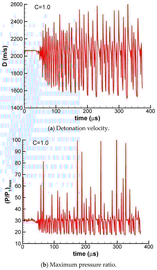
Figure 4. The detonation velocity and maximum pressure of periodic detonation.

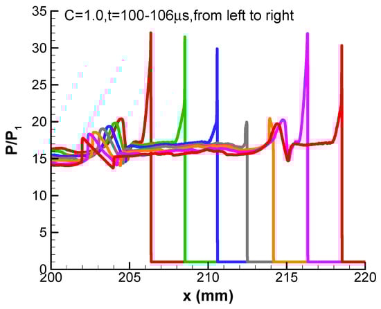
Figure 5. The pressure profiles of periodic detonation.

This periodic behavior can be explained by the flux analysis mythology. The convective fluxes from 100 μs to 105 μs are shown in Figure 6. At t = 100 μs, the heat release is coupled with the shock wave and there are two peaks of heat release. The negative convective flux peak point Γ₁ coincides with the second heat release summit point Q₁ at x = 206.35 mm and counteracts the heat release there. Accordingly, the pressure and temperature there are decreased and the chemical reaction rate becomes slower.

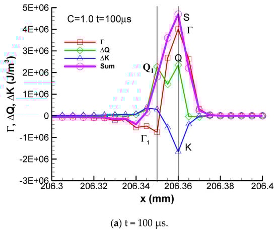
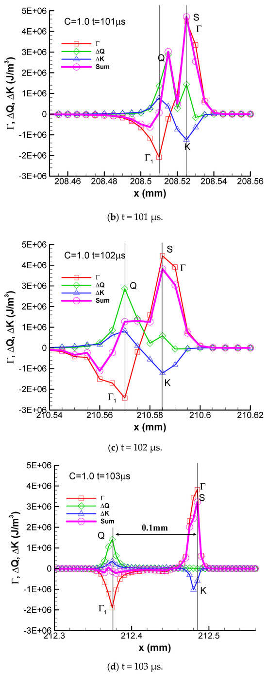
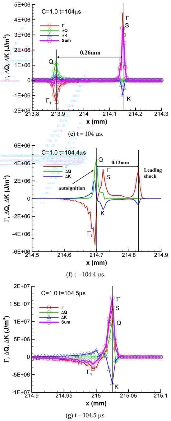
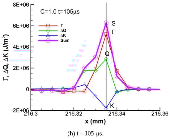
Figure 6. The profiles of convective flux of periodic detonation.

At t= 101 μs, the point Q is two grid points behind the shock wave. The negative convective flux point Γ₁ becomes stronger and is only one grid point behind the heat peak point Q. At t= 102 μs, the negative convective flux point Γ₁ moves forward and is at the same grid point with the point Q at x = 210.57 mm. The total summation of these three fluxes is very small, which means that the internal energy of combustion products does not increase too much, although combustion takes place there. At t = 103 μs and 104 μs, the flame fully decouples from the shock wave. The flame coincides with the negative convective flux and the summation is almost zero. The combustion becomes constant-pressure combustion in a sense at these two instants. The distance between the flame and the shock wave becomes wider as time goes by. However, autoignition occurs at t = 104.4 μs and the flame is recoupled with the shock wave again at t = 104.5 μs. The detonation wave propagates periodically following this mechanism.

3.4. Key Mechanism of Detonation Instability

The above discussion indicates that the negative convective flux plays a crucial role in detonation instability. This negative convective flux is generated by the sharper and steeper enthalpy flux F_E at the detonation front, which is defined in Equation (12). The corresponding enthalpy fluxes of the periodic detonation at different instants are shown Figure 7. We can see from Figure 7 that the gradient of enthalpy flux at detonation front is very large.

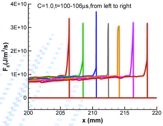
Figure 7. The enthalpy fluxes of periodic detonation.

The reason is that the total enthalpy on the detonation front varies very significantly once the flame is decoupled from the shock wave during detonation propagation. The theoretical total enthalpy on the theoretical C-J detonation point and a Ma4.85 normal shock wave front (Gaseq results) are listed in Table 2. The Ma4.85 is the Mach number of C-J detonation. It can be seen from Table 2 that the total enthalpy of the shock wave front is almost more than four times larger than that of the C-J detonation front. This means that the enthalpy flux becomes much sharper and steeper once the flame is decoupled from the shock wave. Consequently, the sharper and steeper enthalpy flux produces a much stronger negative convective flux, which reduces the total energy per unit volume of detonation products.

Table 2. Theoretical parameters on C-J detonation and shock front.

Parameters	C-J Detonation	Ma4.85 Shock	Ratio
Density (kg/m3)	1.49	4.58	0.32
P (atm)	15	27.9	0.53
T (K)	2956	1548	1.9
Gas velocity (m/s)	849	1612	0.52
Total enthalpy (MJ/m3)	8.19	31.67	0.25

The density profiles and gas velocity profiles of detonation under different activation energy are drawn in Figure 8a,b, respectively. The maximum density and maximum gas velocity on the detonation front increase with the increase in activation energy. Their values are between the theoretical value of C-J detonation and the Ma4.85 normal shock wave theoretical value, consistent with the data in Table 2. These numerical results confirm the key role of convective flux in the detonation instability.

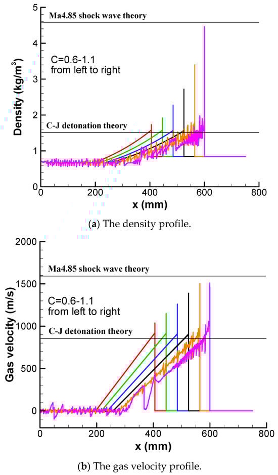
Figure 8. The density and gas velocity profiles under different activation energy.

The numerical results of the enlarged enthalpy flux F_E and the chemical reaction progress parameter Z at t = 103 μs are plotted in Figure 9. It can be found that the combustion induces a significant drop in enthalpy flux. In other words, the system transition from reactants to detonation products leads to the synchronous system transition of enthalpy flux from reactants to combustion products. Therefore, we can find that there is always a negative convective flux accompanying the heat release once the flame is decoupled from the shock wave. This is the intrinsic nature of the one-dimensional reactive Euler system.

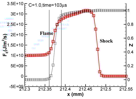
Figure 9. The enlarged enthalpy flux at the detonation front.

The corresponding raw CFD data on the chemical reaction front are presented in Table 3. It can be seen that the enthalpy flux (ρE + p)u of detonation products decreases to be 0.39 times of that of the reactants within a flame thickness of 35 μm. In the sharp decrease in enthalpy flux (ρE + p)u, the contribution of enthalpy (ρE + p) is larger than the contribution of velocity, with contributions of 0.48 times and 0.81 times, respectively. The variation in energy per unit volume ρE plays a more important role than pressure in the variation of enthalpy (ρE + p), by 0.43 times and 0.89 times, respectively. In the energy per unit volume ρE, the density ρ is a very important parameter, which decreases to be 0.51 times that of the reactants. The variation in specific energy E is smaller—0.86 times that of the reactants.

Table 3. Raw CFD data on the periodic detonation front (t = 103 μs).

Parameters	Z2 = 0.000525 (x2 = 212.3549 mm)	Z1 = 0.922388 (x1 = 212.3899 mm)	Ratio
(ρE + p)u (GJ/m2/s)	10.643565098	27.252431740	0.39
(ρE + p) (MJ/m3)	9.8315187701	20.438580481	0.48
u (m/s)	1050.0912067	1289.5199184	0.81
ρE (MJ/m3)	8.0955706013	18.501844005	0.43
p/p1	17.128250308	19.109388017	0.89
E (MJ/kg)	4.7977229115	5.5738917896	0.86
ρ (kg/m3)	1.6873776895	3.3193762461	0.51

3.5. Pulsating Detonation (C = 1.1)

The detonation velocity and maximum pressure ratio of pulsating detonation (C = 1.1) are shown in Figure 10. It can be found that the detonation shows pulsating behavior or chaotic behavior under higher activation energy. The detonation velocity oscillates very violently between 1400 m/s and 2900 m/s, and the maximum pressure ratio oscillates very violently between 15 and 120. Additionally, it looks like the detonation is quenched at about t = 210 μs and the reignition occurs at about t = 220 μs.

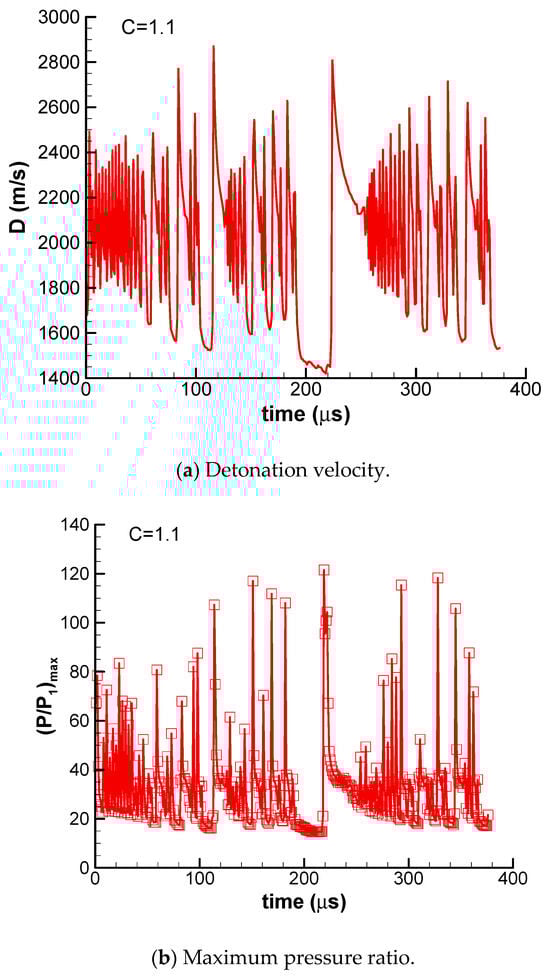
Figure 10. The velocity and maximum pressure ratio of pulsating detonation.

The raw CFD data from t = 216 μs to 225 μs are presented in Table 4. It can be seen that the lowest value of the maximum pressure ratio is 14.7 at t = 217 μs. The maximum pressure ratio reaches the highest value of 121.5 at t = 219 μs. The lowest detonation velocity is 1420 m/s at t = 218 μs. The detonation velocity reaches the highest value of 2807.8 m/s at t = 224 μs, which is 5 μs later than the maximum pressure ratio. Detonation re-initiation takes place at t = 219 μs according to the maximum pressure ratio.

Table 4. Raw CFD data of pulsating detonation.

Time (μs)	Max Pressure Ratio	D (m/s)
216.0013826	14.74804655	1429.370885
217.0001875	14.78441109	1426.704896
218.0000598	21.08271153	1420.181349
219.0000025	121.5199589	1450.083062
220.0003849	95.50619433	1459.441851
221.0002412	100.9162851	1455.20912
222.0003638	104.3333027	1449.822244
223.0000983	67.09051245	1585.420866
224.0008763	47.50537086	2807.815416
225.000231	44.0902092	2691.737026

The profiles of flux and pressure gain of pulsating detonation at t = 217 μs are plotted in Figure 11. We can find from Figure 11a that the flame is completely decoupled from the shock front at this instant. The shock wave is at x = 426 mm, the flame front is at x = 418.6 mm, and the distance between them is about 8 mm. The local enlarged profiles of fluxes are shown in Figure 11b. The pressure gain at the flame front shown in Figure 11c is almost negative, which means that the combustion cannot generate positive pressure to support the shock wave propagation. These results reveal that the negative convective flux is the key mechanism of detonation quenching.

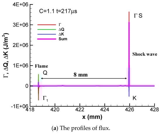
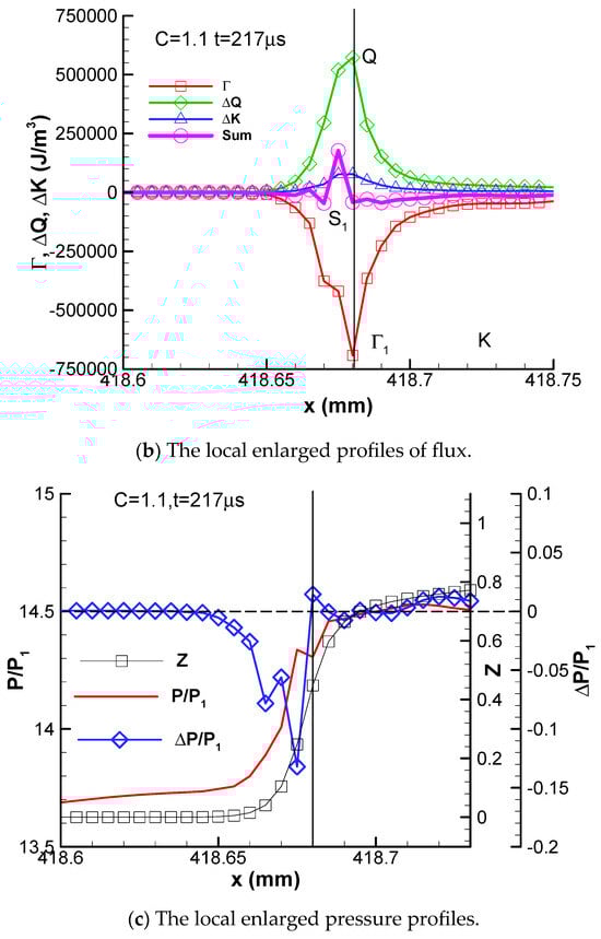
Figure 11. The profiles of flux at t = 217 μs of pulsating detonation.

The profiles of flux at t = 218 μs are plotted in Figure 12. The flame is still decoupled from the shock wave at this instant. However, a new positive convective flux or a hotspot emerges in front of the flame at x = 420.6 mm, which is shown clearly in Figure 12b. This local hotspot increases the total energy per unit volume due to compression waves, rather than combustion heat release. No heat is released at this hotspot at this instant because the Z profile is flat there. As a result, the local pressure and temperature are increased by this compression wave, as shown in Figure 12c. Figure 12c reveals that the compression wave generates a positive pressure gain of about 0.16 atm at x = 420.6 mm. Autoignition induced by this hotspot occurs at the next time step.

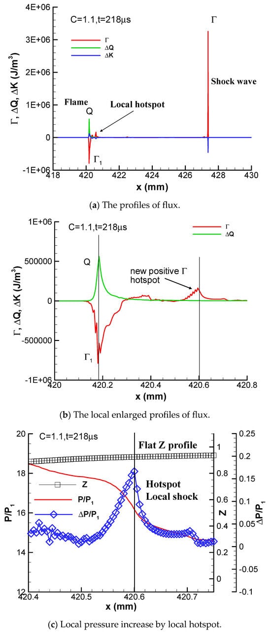
Figure 12. The profiles of flux at t = 218 μs of pulsating detonation.

The profiles of enthalpy flux of pulsating detonation at the instant of t = 217 μs and 218 μs are given in Figure 13. We can see from Figure 13 that the enthalpy profiles of pulsating detonation become jagged and the local slope is negative. The local negative slope of enthalpy flux at t = 218 μs produces a positive convective flux at about x = 420.6 mm, which serves as a local compression wave or a local hotspot for detonation reinitiation. This hotspot triggers detonation reignition at t = 219 μs, occurring at x = 422.3 mm, approximately 7 mm behind the leading shock wave, as shown in Figure 14. It can be seen from Figure 14c that the reignition produces a pressure gain of 30 atm and the pressure spike increases to 120 atm. An overdriven detonation is formed when this reignition detonation catches up with the leading shock wave. This is the governing mechanism of pulsating detonation.

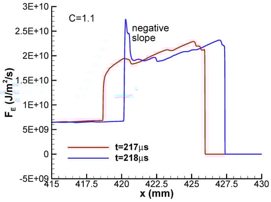
Figure 13. The profiles of enthalpy flux of pulsating detonation.

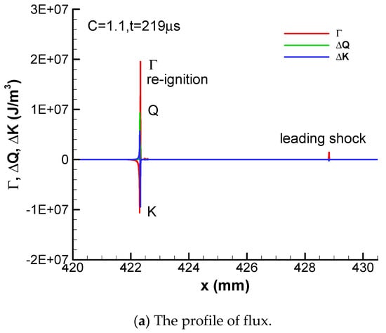
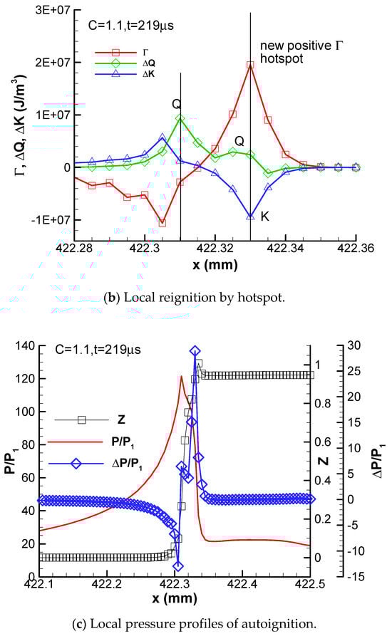
Figure 14. The profiles of flux at t = 219 μs of pulsating detonation.

The key distinction between periodic detonation (C = 1.0) and pulsating detonation (C = 1.1) lies in their governing mechanisms. Periodic detonation is driven by the decoupling and recoupling of flame and shock waves, whereas pulsating detonation results from detonation quenching followed by the reignition of a new detonation wave behind a decaying leading shock wave.

3.6. The Decaying Mechanism of Overdriven Detonation

The formation and decaying process of overdriven detonation from t = 222 μs to 225 μs is plotted in Figure 15. It can be seen that the reignition detonation is about 1.8 mm behind the leading shock wave at t = 222 μs. This reignition detonation catches up with the leading shock wave and an overdriven detonation is formed at t = 223 μs and 224 μs. This overdriven detonation reaches its highest velocity value of 2807.8 m/s at this instant. However, the premature combustion occurs on the windward side of the shock wave and decreases the strength of overdriven detonation gradually. Finally, the pulsating detonation becomes non-overdriven at t = 225 μs. The premature combustion is the decaying mechanism of an overdriven detonation.

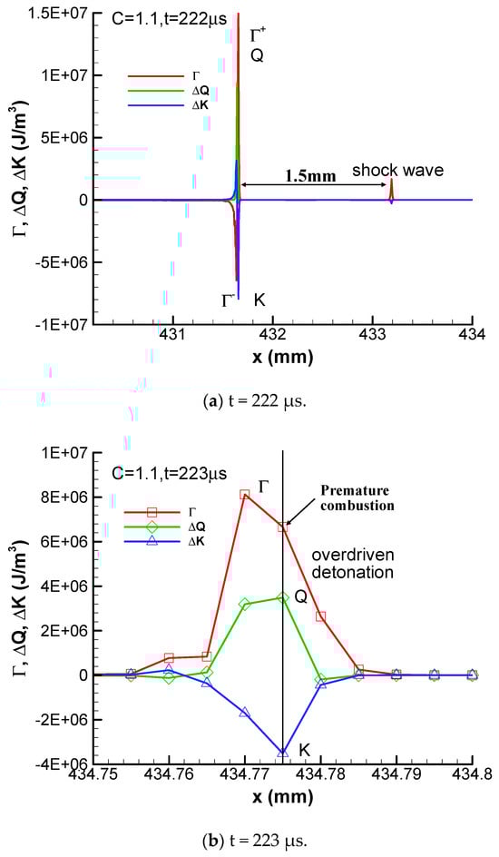
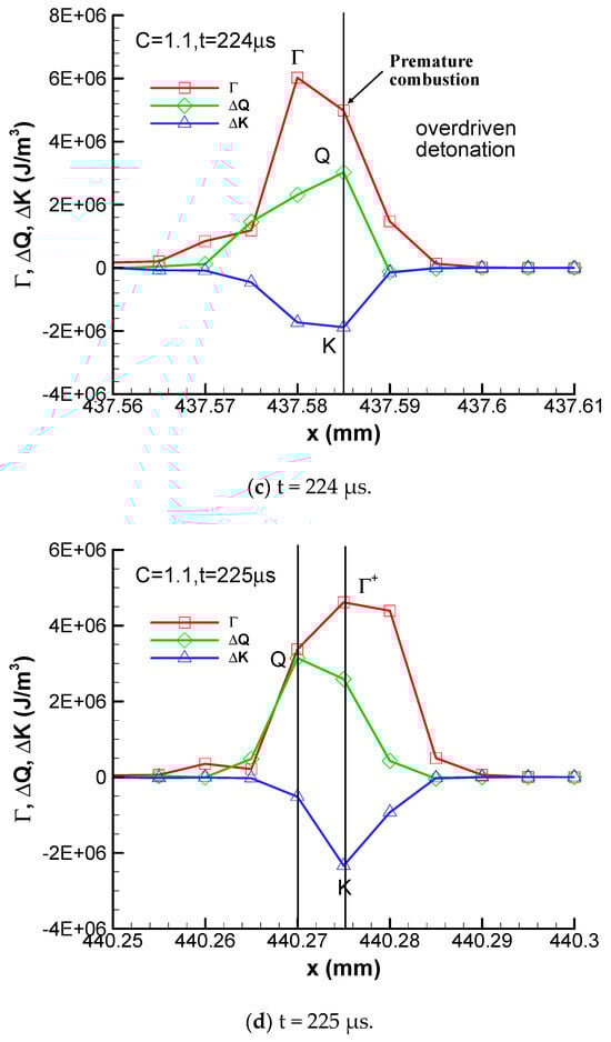
Figure 15. The decaying process of overdriven detonation.

4. Verification and Resolution Study

4.1. Code Verification

This homemade code was successfully used to simulate detonation in previous studies [30,31]. In this verification study, its capacity to simulate detonation instability is checked and compared with references. The C-J detonation parameters of CFD and theoretical results are listed in Table 5. This code can simulate C-J conditions quantitatively. An ignition delay time comparison of this one-step model (activation energy C = 1.0) with experimental results [32,33,34] and a detailed model [35] of the stoichiometric H₂–air mixture is plotted in Figure 16, which demonstrates that this one-step model can simulate the ignition delay time correctly. Two-dimensional numerical simulations are performed to simulate the detonation cell structure (activation energy C = 1.0) and the results are shown in Figure 17. The average length and width of the detonation cell are 12 mm and 8 mm, respectively, which is in good agreement with the experimental results of 15.4 mm and 8 mm, quantitatively [36].

Table 5. CFD and theoretical results of C-J condition.

Parameters	CFD	Theory (Gaseq)	Ratio
Density (kg/m3)	1.54	1.49	1.03
P (atm)	15.82	15.08	1.04
T (K)	2986	2956	1.01
Gas velocity (m/s)	890	849	1.05
D (m/s)	1982	1979	1.01

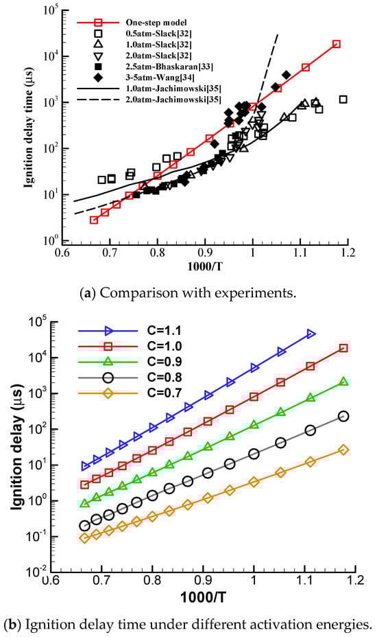
Figure 16. Ignition delay time comparison of one-step model with experiments.

Figure 17. The detonation cell structures simulated by a one-step model.

The nonlinear dynamical behavior of one-dimensional detonation was numerically simulated with Euler equations and one-step Arrhenius kinetics by Ng et al. [19]. Their study showed a strong similarity between one-dimensional periodic detonation and simple nonlinear dynamical systems. The maximum pressure ratio of periodic detonation wave (C = 1.0) of this study (red line) is compared with that of Ref. [19] in Figure 18. In addition, the maximum pressure ratio of pulsating detonation (C = 1.1) is compared with that of Ref. [26] in Figure 19. Good agreements are achieved qualitatively.

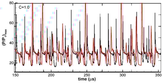
Figure 18. Comparison of the maximum pressure ratio of the present study (red line) with that of Ref. [19].

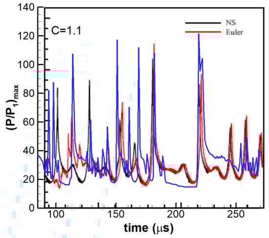
Figure 19. Comparison of the maximum pressure ratio of the present study (blue line) with that of Ref. [26].

4.2. Resolution Study

This study reveals that the convective flux plays an important role in the detonation instability. The aim of this resolution study is to demonstrate that this conclusion holds under different grid sizes. The resolution study with a uniform grid size of 2.5 μm was conducted and the velocity under different activation energies is plotted in Figure 20. It can be seen that the three regions of detonation propagation mode—a stable region (C = 0.8–0.9), an unstable region (C = 1.0–1.1), and a quenching region (C ≥ 1.15)—are reproduced successfully.

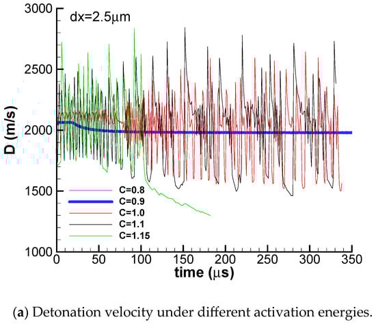
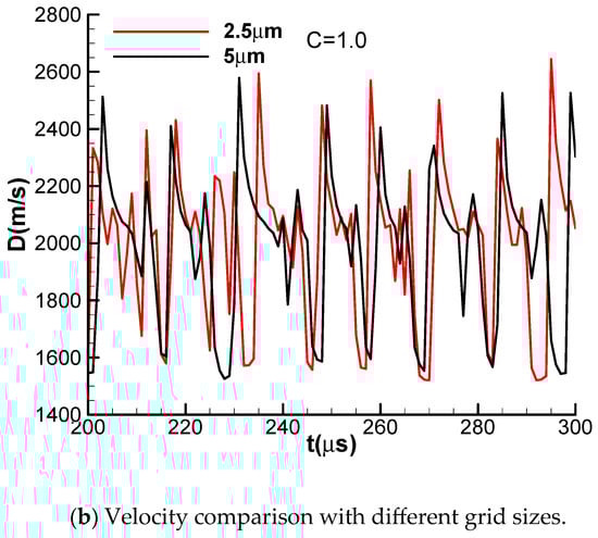
Figure 20. Detonation velocity with a grid size of 2.5 μm.

5. Conclusions

One-dimensional numerical simulations with Euler equations and irreversible one-step Arrhenius kinetics are performed to study the underlying physics of the instability of one-dimensional gaseous detonation. The theoretical equation of pressure gain of detonation products within one time step is deduced. The stable detonation, the pulsating detonation, and the detonation quenching process are obtained successfully by increasing the activation energy in the numerical simulations. This study comes to the following conclusions.

(1)

The theoretical pressure gain equation identifies three key parameters governing detonation propagation: convective flux, kinetic energy flux, and chemical reaction heat release. The pressure gain or the internal energy gain of detonation products are attributed to the algebra summation of these three fluxes.

(2)

The detonation is stable under lower activation energy. The heat release flux is tightly coupled with the shock wave and almost 100% of heat is released on the windward side of the shock wave because of the very fast chemical reaction rate under lower activation energy. The stable detonation is a form of constant-volume combustion.

(3)

The detonation becomes unstable, pulsating, and chaotic with the increase in activation energy. The flame is completely decoupled from the shock wave for the unstable detonation. The negative convective flux at the flame front reduces the total energy per unit volume of combustion products, effectively resulting in a constant-pressure combustion mode.

(4)

The negative convective flux plays a key role in the detonation instability and detonation quenching process, which decreases the internal energy of detonation products. The negative convective flux is produced by the sharper and steeper enthalpy flux at the detonation front, whose slope becomes very big once the flame is decoupled from the shock wave.

(5)

The sharper and steeper enthalpy flux is produced by the significant variation in physical parameters at the von Neumann and C-J detonation points. Once the flame decouples from the shock wave, the enthalpy flux in the von Neumann spike increases by an order of magnitude, inducing a much stronger negative convective flux or rarefaction wave, which suppresses the pressure gain generated by heat release.

References

- Lee, J.H. The Detonation Phenomenon; Cambridge University Press: Cambridge, UK, 2008. [Google Scholar]
- Erpenbeck, J.J. Stability of steady-state equilibrium detonations. Phys. Fluids 1962, 5, 604. [Google Scholar] [CrossRef]
- Erpenbeck, J.J. Structure and stability of the square-wave detonation. Symp. (Int.) Combust. 1963, 9, 442. [Google Scholar] [CrossRef]
- Erpenbeck, J.J. Stability of idealized one-reaction detonations. Phys. Fluids 1964, 7, 684. [Google Scholar] [CrossRef]
- Lee, H.I.; Stewart, D.S. Calculation of linear detonation instability: One-dimensional instability of plane detonation. J. Fluid Mech. 1990, 216, 103. [Google Scholar] [CrossRef]
- Sharpe, G.J. Linear stability of idealized detonations. Proc. R. Soc. Lond. Ser. A 1997, 453, 2603. [Google Scholar] [CrossRef]
- Short, M. Multidimensional linear stability of a detonation wave at high activation energy. SIAM J. Appl. Math. 1997, 57, 307–326. [Google Scholar] [CrossRef]
- Short, M. A parabolic linear evolution equation for cellular detonation instability. Combust. Theory Model. 1997, 1, 313–346. [Google Scholar] [CrossRef]
- Gorchkov, V.; Kiyanda, C.B.; Short, M.; Quirk, J.J. A detonation stability formulation for arbitrary equations of state and multi-step reaction mechanisms. Proc. Combust. Inst. 2007, 31, 2397. [Google Scholar] [CrossRef]
- Uy, K.C.K.; Shi, L.; Hao, J.; Wen, C.-Y. Linear stability analysis of one-dimensional detonation coupled with vibrational relaxation. Phys. Fluids 2020, 32, 126101. [Google Scholar] [CrossRef]
- Xu, Z.; Dong, G.; Wang, Y. A study of pulsating behavior and stability parameter for one-dimensional non-ideal detonations. Phys. Fluids 2023, 35, 016101. [Google Scholar] [CrossRef]
- Sharpe, G.J.; Falle, S.A.E.G. One-dimensional numerical simulations of idealized detonations. Proc. R. Soc. Lond. Ser. A 1999, 455, 1203. [Google Scholar] [CrossRef]
- Sharpe, G.J.; Falle, S.A.E.G. Numerical simulations of pulsating detonations: I. Nonlinear stability of steady detonations. Combust. Theory Model. 2000, 4, 557. [Google Scholar] [CrossRef]
- Sharpe, G.J. Numerical simulations of pulsating detonations: II. Piston initiated detonations. Combust. Theory Model. 2001, 5, 623. [Google Scholar] [CrossRef]
- Short, M.; Quirk, J.J. On the nonlinear stability and detonability limit of a detonation wave for a model three-step chain-branching reaction. J. Fluid Mech. 1997, 339, 89–119. [Google Scholar] [CrossRef]
- Short, M.; Sharpe, G. Pulsating instability of detonations with a two-step chain-branching reaction model: Theory and numerics. Combust. Theory Model. 2003, 7, 401. [Google Scholar] [CrossRef]
- Hwang, P.; Fedkiw, R.P.; Merriman, B.; Aslam, T.D.; Karagozian, A.R.; Osher, S.J. Numerical resolution of pulsating detonation waves. Combust. Theory Model. 2000, 4, 217–240. [Google Scholar] [CrossRef]
- Ng, H.D.; Radulescu, M.I.; Higgins, A.J.; Nikiforakis, N.; Lee, J.H.S. Numerical investigation of the instability for one-dimensional Chapman-Jouguet detonations with chain-branching kinetics. Combust. Theory Model. 2005, 9, 385–401. [Google Scholar] [CrossRef]
- Ng, H.D.; Higgins, A.J.; Kiyanda, C.B.; Radulescu, M.I.; Lee, J.H.S.; Bates, K.R.; Nikiforakis, N. Non-linear dynamics and chaos analysis of one-dimensional pulsating detonations. Combust. Theory Model. 2005, 9, 159–170. [Google Scholar] [CrossRef]
- Kasimov, A.R.; Stewart, D.S. On the dynamics of self-sustained one-dimensional detonations: A numerical study in the shock-attached frame. Phys. Fluids 2004, 16, 3566–3578. [Google Scholar] [CrossRef]
- Henrick, A.K.; Aslam, T.D.; Powers, J.M. Simulations of pulsating one-dimensional detonations with true fifth order accuracy. J. Comput. Phys. 2006, 213, 311–329. [Google Scholar] [CrossRef]
- Powers, J.M. Review of multiscale modeling of detonation. J. Propul. Power 2006, 22, 1217–1229. [Google Scholar] [CrossRef]
- Choi, J.Y.; Ma, F.H.; Yang, V. Some numerical issues on simulation of detonation cell structures. Combust. Expl. Shock Waves 2008, 44, 560–578. [Google Scholar] [CrossRef]
- Sharpe, G.J.; Radulescu, M.I. Statistical analysis of cellular detonation dynamics from numerical simulations: One-step chemistry. Combust. Theory Model. 2011, 15, 691–723. [Google Scholar] [CrossRef]
- Han, W.; Gao, Y.; Wang, C.; Law, C.K. Coupled pulsating and cellular structure in the propagation of globally planar detonations in free space. Phys. Fluids 2015, 27, 106101. [Google Scholar] [CrossRef]
- Han, W.; Wang, C.; Law, C.K. Pulsation in one-dimensional H2-O2 detonation with detailed reaction mechanism. Combust. Flame 2019, 200, 242–261. [Google Scholar] [CrossRef]
- Zhu, R.; Fang, X.; Xu, C.; Zhao, M.; Zhang, H.; Davy, M. Pulsating one-dimensional detonation in ammonia-hydrogen-air mixtures. Int. J. Hydrogen Energy 2022, 47, 21517–21536. [Google Scholar] [CrossRef]
- Liu, Y. The thermodynamics of C-J deflagration. Case Stud. Therm. Eng. 2024, 64, 105574. [Google Scholar] [CrossRef]
- Ma, F.; Choi, J.Y.; Yang, V. Thrust chamber dynamics and propulsive performance of single-tube pulse detonation engines. J. Propuls. Power 2005, 21, 512–526. [Google Scholar] [CrossRef]
- Liu, Y.F.; Jiang, Z. Reconsideration on the role of the specific heat ratio in Arrhenius law applications. Acta Mechnica Sin. 2008, 24, 261–266. [Google Scholar] [CrossRef]
- Liu, Y.F.; Zhang, W.; Jiang, Z. Relationship between ignition delay time and cell size of H2-air detonation. Int. J. Hydrogen Energy 2016, 41, 11900–11908. [Google Scholar] [CrossRef]
- Slack, M.W. Rate coefficient for H + O2 + M = HO2 + M evaluated from shock tube measurements of induction times. Combust. Flame 1977, 28, 241–249. [Google Scholar] [CrossRef]
- Bhaskaran, K.A.; Gupta, M.C.; Just, T. Shock tube study of the effect of unsymmetric dimethyl hydrazine on the ignition characteristics of hydrogen-air mixtures. Combust. Flame 1973, 21, 45–48. [Google Scholar] [CrossRef]
- Wang, B.L.; Olivier, H.; Grönig, H. Ignition of shock-heated H2-air-steam mixtures. Combust. Flame 2003, 133, 93–106. [Google Scholar] [CrossRef]
- Jachimowski, C.J. An analytical study of the hydrogen–air reaction mechanism with application to scramjet combustion. NASA TP 2791; 1988. Available online: https://ntrs.nasa.gov/citations/19880006464 (accessed on 17 November 2025).
- Kaneshige, M.; Shepherd, J.E. Detonation database. Technical Report FM97-8, GALCIT. July 1997. Available online: https://shepherd.caltech.edu/detn_db/html/db.pdf (accessed on 17 November 2025).
Disclaimer/Publisher’s Note: The statements, opinions and data contained in all publications are solely those of the individual author(s) and contributor(s) and not of MDPI and/or the editor(s). MDPI and/or the editor(s) disclaim responsibility for any injury to people or property resulting from any ideas, methods, instructions or products referred to in the content. |
© 2025 by the author. Licensee MDPI, Basel, Switzerland. This article is an open access article distributed under the terms and conditions of the Creative Commons Attribution (CC BY) license (https://creativecommons.org/licenses/by/4.0/).