Article

Adaptive Strategy for the Path Planning of Fixed-Wing UAV Swarms in Complex Mountain Terrain via Reinforcement Learning

1
School of Space Science and Technology, Xidian University, Xi’an 710118, China
2
Xi’an ASN Technology Group Co., Ltd., Xi’an 710065, China
3
365th Research Institute, Northwestern Polytechnical University, Xi’an 710072, China
*
Author to whom correspondence should be addressed.
Aerospace 2025, 12(11), 1025; https://doi.org/10.3390/aerospace12111025
Submission received: 9 October 2025 / Revised: 17 November 2025 / Accepted: 18 November 2025 / Published: 19 November 2025
(This article belongs to the Special Issue Formation Flight of Fixed-Wing Aircraft)

Abstract

Cooperative path planning for multiple Unmanned Aerial Vehicles (UAVs) within complex mountainous terrain presents a unique challenge, characterized by a high-dimensional search space fraught with numerous local optima. Conventional metaheuristic algorithms often fail in such deceptive landscapes due to premature convergence stemming from a static balance between exploration and exploitation. To overcome the aforementioned limitations, this paper develops the Reinforcement Learning-guided Hybrid Sparrow Search Algorithm (RLHSSA), an optimization framework specifically engineered for robust navigation in complex topographies. The core innovation of RLHSSA lies in its two-level architecture. At a lower level, a purpose-built operator suite provides specialized tools essential for mountain environments: robust exploration strategies, including Levy Flight, to escape the abundant local optima, and an Elite-SSA for the high-precision exploitation needed to refine paths within narrow corridors. At a higher level, a reinforcement learning agent intelligently selects the most suitable operator to adapt the search strategy to the terrain’s complexity in real-time. This adaptive scheduling mechanism is the key to achieving a superior exploration–exploitation balance, enabling the algorithm to effectively navigate the intricate problem landscape. Extensive simulations within challenging mountainous environments demonstrate that RLHSSA consistently outperforms state-of-the-art algorithms in solution quality and stability, validating its practical potential for high-stakes multi-UAV mission planning.

1. Introduction

Unmanned aerial vehicles (UAVs) have achieved remarkable advancements and are now broadly employed across various fields, including surveillance, agriculture, and environmental monitoring [1,2,3]. Compared to traditional manned-aircraft platforms, UAVs offer unparalleled flexibility and can collect high spatial and temporal resolution data at lower cost by operating at low altitudes [4]. However, deploying UAVs for missions in complex and challenging environments presents significant difficulties [5]. Mountainous areas, for instance, are characterized by intricate terrain, steep slopes, and varying altitudes, which pose substantial obstacles to safe and efficient flight [6]. Successful mission execution in complex, hazardous environments depends on the UAV’s autonomous and safe navigation [7,8].
For many UAV tasks, utilizing a single UAV may be inefficient, especially when covering large areas [9,10]. In such scenarios, multi-UAV systems offer distinct advantages for rapid data acquisition, including enhanced coverage, reduced mission time, and increased robustness through cooperation [11,12,13]. Nevertheless, navigating a swarm of UAVs through complex 3D terrain—while ensuring collision avoidance with terrain, obstacles, and each other, and simultaneously considering threats and other operational constraints—presents a formidable navigation challenge [14,15,16]. Therefore, developing effective cooperative path planning strategies is a critical requirement for advancing UAV capabilities in challenging real-world applications.
The challenge of multi-UAV cooperative path planning within intricate environments remains a focal point of research. Solutions can often be broadly categorized into traditional methods, such as graph-based search algorithms (e.g., A* [17], Dijkstra [18]) and sampling-based methods (e.g., rapidly exploring random trees [19]), alongside optimization-based techniques including mathematical programming and metaheuristic algorithms [20,21,22]. While traditional methods are effective in well-defined or lower-dimensional spaces, they often face scalability issues and computational challenges when applied to high-dimensional, continuous, and complex 3D environments with numerous obstacles and constraints, which are typical of realistic mountainous terrains. Optimization-based methods, particularly metaheuristic algorithms including genetic algorithms (GAs) [23], particle swarm optimization (PSO) [24], and grey wolf optimizer (GWO) [25], have shown promise in handling complex search spaces and multiple objectives. For example, Zhang et al. [26] enhanced the differential evolution (DE) algorithm through the integration of multiple strategies, proposing a novel variant, namely MSIDE. This method was specifically tailored for UAV 3D path planning in challenging mountainous scenarios, aiming to provide effective solutions for this intricate problem. Meng et al. [27] developed an evolutionary state estimation-based multi-strategy jellyfish search (ESE-MSJS) algorithm to address path planning for multiple UAVs in intricate environments. Their approach integrates a switching framework based on evolutionary state estimation and employs various learning strategies to enhance search efficiency and adapt to complex constraints.
Furthermore, reinforcement learning (RL) provides an effective methodology where an agent acquires optimal actions or strategies by interacting with its surroundings, aiming to maximize cumulative rewards [28]. RL has gained significant attention in various fields, including robotics, control, and intelligent decision making [29]. Researchers have explored integrating RL with optimization algorithms to enhance their search capabilities or adapt their parameters during the optimization process [30,31].
However, directly applying standard metaheuristic algorithms to this multi-UAV routing task reveals a critical vulnerability when faced with the unique topography of mountainous environments. Such landscapes create a deceptive search space characterized by numerous local optima and narrow, winding feasible corridors. A key limitation of conventional methods is their reliance on a static or overly simplistic adaptive balance between exploration and exploitation [32,33]. This inflexibility renders them prone to premature convergence within a suboptimal valley or inefficiently searching after a viable corridor has been found. These challenges highlight the urgent need for a more intelligent optimization paradigm that can dynamically adapt its search behavior to the specific topographical complexities it encounters.
To conquer these topographical challenges, we introduce a novel optimization framework: the Reinforcement Learning-guided Hybrid Sparrow Search Algorithm (RLHSSA). The primary innovation of RLHSSA is to replace the fixed search strategy of the standard Sparrow Search Algorithm (SSA) [34] with a learning-based, two-level architecture. Specifically, we enhance the SSA foundation by integrating a purpose-built suite of operators; powerful exploration strategies, including Adaptive Differential Perturbation and Levy Flight, are incorporated to provide the long-jump capability necessary to escape the numerous local optima inherent in mountain landscapes. Simultaneously, an Elite-SSA operator provides the high-precision exploitation required to refine trajectories within narrow, viable corridors. The entire process is governed by an RL-based scheduling mechanism.
More importantly, the RL-based strategy scheduling mechanism allows the algorithm to intelligently select the most suitable operator throughout the optimization process based on feedback from the search environment. This adaptive strategy selection is expected to enable RLHSSA to better balance exploration and exploitation, adapt to different search stages, and effectively navigate the complex, high-dimensional search space associated with multi-UAV cooperative path planning in challenging mountainous and threatened environments. In summary, this paper makes the following key contributions:
(1)
A novel Reinforcement Learning-guided Hybrid Sparrow Search Algorithm (RLHSSA) is proposed. This algorithm uniquely combines a base metaheuristic (SSA) with a suite of specialized operators and an adaptive RL framework to address complex multi-UAV path planning challenges, offering a more robust and efficient solution than single-strategy or non-adaptive approaches.
(2)
Three distinct optimization operators—the Elite-SSA, the Adaptive Differential Perturbation strategy, and the Adaptive Levy Flight strategy—are designed and integrated into the framework. This integration provides a rich set of search behaviors, with Elite-SSA focusing on refined exploitation while the other two operators enhance search diversity and global exploration, thereby mitigating the common issue of premature convergence.
(3)
A novel reinforcement learning-based mechanism is developed for the dynamic scheduling of distinct optimization operators within a hybrid metaheuristic. Unlike fixed-strategy or simpler adaptive methods, this mechanism enables the algorithm to intelligently select the most appropriate search behavior for the current optimization phase, leading to a superior exploration–exploitation balance and adaptability.
(4)
Comprehensive simulation experiments and comparative studies were conducted to assess the effectiveness of the RLHSSA method against state-of-the-art methods in both threat-free and threatened environments. Our findings demonstrate RLHSSA’s superior effectiveness concerning convergence speed, solution quality, and robustness, particularly in challenging mountainous scenarios.
The structure of this work is outlined as follows: Section 2 formulates the cooperative path planning problem for multiple UAVs, including the environment modeling and path representation. Section 3 focuses on constructing the problem model for mountainous terrain. Section 4 details the proposed RLHSSA algorithm. Section 5 discusses the simulation settings, experimental outcomes, and corresponding analysis across various scenarios. Finally, Section 6 presents conclusions and future works.

2. Problem Statement

Environmental modeling is a prerequisite for UAV path planning. For multi-UAV operations, the search space is defined by a mathematical representation of the operational environment. The undulating natural terrain in mountainous environments is modeled using an exponential function [24], whose mathematical formulation is provided below: 
Z ( x , y ) = j = 1 m h j exp x x j x s j 2 y y j y s j 2 .
Here, ( x j , y j ) denotes the position of the j-th mountain peak, while h j defines its elevation parameter. The values x s j and y s j control the gradient attenuation along the x- and y-axes, respectively, thereby influencing the steepness of the peak. Furthermore, m indicates the total count of mountain peaks. The environmental model constructed based on Equation (1) is shown in Figure 1a.
To ensure flight, UAVs must consider various potential threats during flight. This paper primarily considers two types of path threats: enemy threat sources and no-fly zones (NFZs). Enemy threat sources include radar, anti-aircraft guns, missiles, and electronic jamming, all of which have different detection ranges of interference strengths. NFZs are areas where flight is prohibited, designated by authorities. To simplify the calculation, we approximate enemy threat sources as hemispheres, with the radius representing the influence range of the threat. NFZs are modeled as cylinders, and a large penalty is imposed if the UAV enters the cylinder. In the model presented in this paper, we assume that the positions of all threat sources and NFZs, as well as their influence ranges, are known in advance. Figure 1b illustrates the 3D environmental model, which incorporates the previously described mountainous terrain and threat sources.

Path Representation

In this system, N represents the total count of UAVs. For any UAV i in the formation ( i = 1 , 2 , , N ) , it needs to fly from the start point S i : ( x i , s , y i , s , z i , s ) to the end point T i : ( x i , e , y i , e , z i , e ) . The flight path is composed of M waypoints, denoted as p i , j : ( x i , j , y i , j , z i , j ) , j = 1 , 2 , , M . To simplify the modeling process, we define p i , 0 : = S i , p i , M + 1 : = T i . Thus, the route of UAV i is denoted by P i = { p i , 0 , p i , 1 , , p i , M , p i , M + 1 } . Subsequently, the system’s complete trajectory is given as P a t h = { P 1 , P 2 , , P N } .

3. Multi-UAV Cooperative Path Planning

3.1. Flight Distance Cost

In this work, each UAV is modeled as a point-mass kinematic agent. For UAV i, the path segment formed by two consecutive waypoints p i , j and p i , j + 1 on its flight path is represented as p i , j p i , j + 1 . For convenience, we define L i , j : = p i , j p i , j + 1 . The corresponding distance of this segment is computed as L i , j . The flight distance cost function F 1 is:
F 1 ( P a t h ) = i = 1 N j = 0 M L i , j .

3.2. Flight Altitude Cost

Within the domain of 3D multi-UAV path planning, higher flight altitudes increase UAV susceptibility to enemy radar detection, whereas lower altitudes heighten the risk of collision with the ground. Therefore, the flight altitude of UAVs must be set within a safe range, and altitude changes should be minimized during flight to ensure flight safety. The flight altitude cost function is given by:
C o s t i , j = | z i , j + 1 z i , j | , if H min ( z i , j , z i , j + 1 ) H max , otherwise
F 2 ( P a t h ) = i = 1 N j = 0 M C o s t i , j ,
where H min and H max correspond to lowest and highest allowable altitudes for the UAV. The values z i , j and z i , j + 1 are the z-axis positions for the UAV i at its j-th and ( j + 1 ) -th waypoints, respectively.

3.3. Path Stability Cost

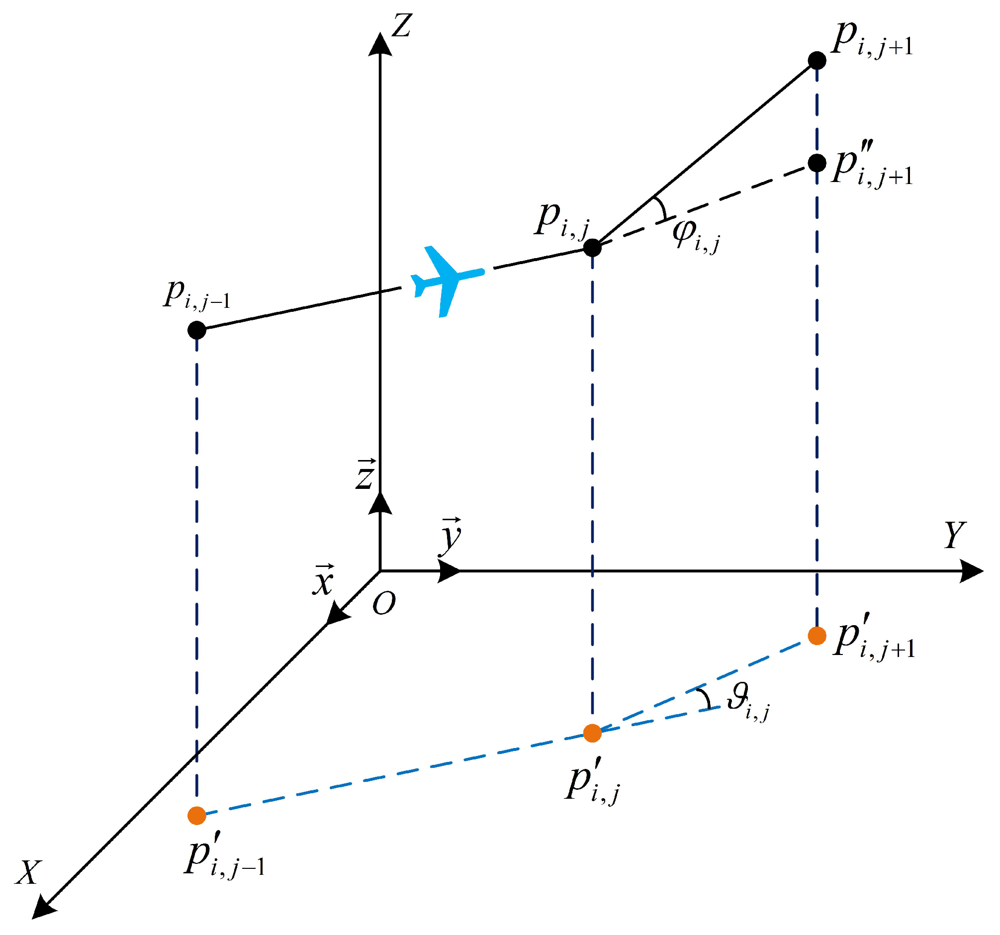
As illustrated in Figure 2, when a UAV maneuvers between path nodes, large turning and climbing angles increase flight instability. Consequently, maintaining an appropriate distance between path nodes is vital for path rationality and stability; overly close nodes, for instance, would necessitate frequent attitude adjustments to meet multiple sequential waypoints quickly.
(1)
Turning angle and Climbing angle
The turning angle cost function of the UAV is calculated as follows:
ϑ i , j = arccos L i , j 1 · L i , j L i , j 1 L i , j
L i , j 1 : = p i , j 1 p i , j , L i , j : = p i , j p i , j + 1
f T ( ϑ i , j ) : = ϑ i , j , if ϑ i , j > ϑ max 0 , otherwise
where ϑ i , j signifies the turning angle of UAV i at its j-th waypoint, and ϑ max is the maximum turning angle of the UAV; L i , j 1 and L i , j are the projection vectors of L i , j 1 and L i , j onto the horizontal plane, respectively.
The climbing angle cost function of the UAV is [31]
φ i , j = arctan z i , j + 1 z i , j L i , j
f C ( φ i , j ) : = | φ i , j φ i , j 1 | , if | φ i , j φ i , j 1 | > φ max 0 , otherwise
where φ i , j denotes the climb angle of UAV i at waypoint j, and φ max specifies the upper bound of permissible climb angle change for the UAV.
The cost function concerning UAV angular variations is:
Angle i , j : = i = 1 N j = 1 M f T ( ϑ i , j ) + i = 1 N j = 1 M f C ( φ i , j )
The path stability cost function is given by:
F 3 ( P a t h ) = Angle i , j .

3.4. Path Threat Cost

(1)
Enemy threat sources
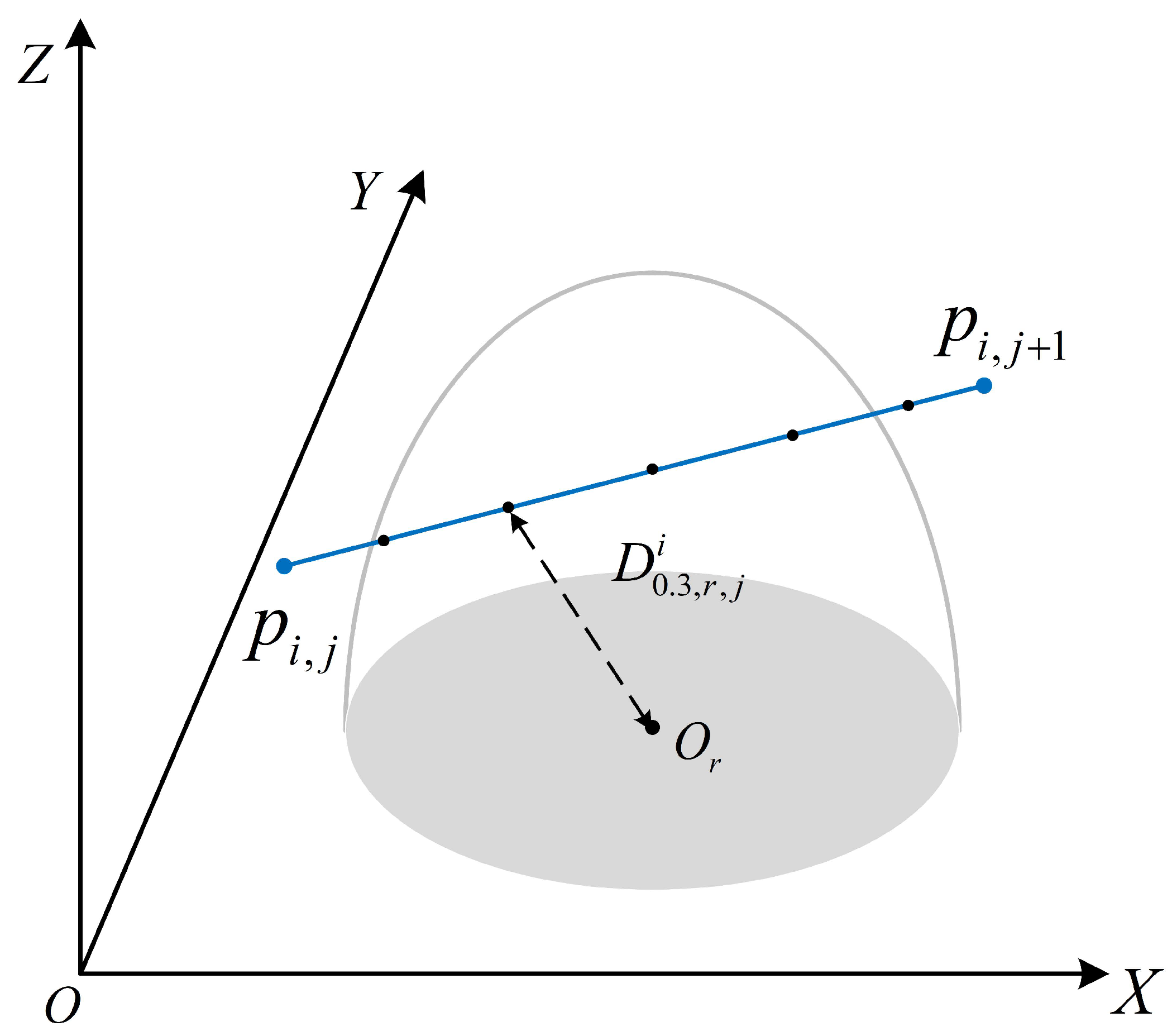
Assume that there are K 1 enemy threat sources in the environment, denoted as O 1 , O 2 , , O r , , O K 1 . Each threat source O r is modeled as a hemispherical influence region with center C r and detection radius d r , i.e.,
O r = { p 3 | p C r d r } .
For a given flight segment L i , j , we say that it is affected by threat source O r if and only if it passes through this influence region, i.e., L i , j O r Ø . As shown in Figure 3, to calculate the threat cost, five sub-nodes are extracted on each flight segment, located at positions 0.1, 0.3, …, and 0.9 along the segment [35]. The enemy threat source cost is calculated as follows:
C j , r i : = G r · 1 D 0.1 , r , j i d r + 1 D 0.3 , r , j i d r + + 1 D 0.9 , r , j i d r , L i , j O r Ø 0 , otherwise
f E ( L i , j ) : = L i , j 10 · r = 1 K 1 C j , r i
F t h r e a t ( P a t h ) : = i = 1 N j = 0 M f E ( L i , j )
The threat level of the r-th threat source is signified by G r , and D 0.1 , r , j i is defined as the distance from the center of threat source O r to the subnode at the 0.1 position on the jth flight segment of UAV i.
(2)
No-fly zones
Assume that there are K 2 no-fly zones in the environment. The u-th no-fly zone is denoted by J u , where u { 1 , 2 , , K 2 } . Each no-fly zone J u is modeled as a vertical cylindrical forbidden region characterized by its horizontal center ( x u N F Z , y u N F Z ) , radius R u N F Z , and height interval [ z min u , z max u ] . The cylindrical region is defined as:
J u = ( x , y , z ) 3 | ( x x u N F Z ) 2 + ( y y u N F Z ) 2 ( R u N F Z ) 2 , z min u z z max u .
For a given flight segment L i , j , we say that it enters the NFZ J u if and only if L i , j J u Ø . The corresponding NFZ penalty for segment L i , j is computed as [36]
ω j , u i : = P N F Z × l i , j , L i , j J u Ø 0 , otherwise
f N ( L i , j ) : = u = 1 K 2 ω j , u i ,
F N F Z ( P a t h ) : = i = 1 N j = 0 M f N ( L i , j ) ,
where P N F Z denotes the penalty coefficient for no-fly zones, and l i , j specifies the length of flight segment L i , j that passes through the no-fly zone J k .
The comprehensive threat cost is formulated as:
F 4 ( P a t h ) : = F t h r e a t ( P a t h ) + F N F Z ( P a t h )

3.5. Terrain Collision Threat Cost

In order to avoid collisions with mountains, when navigating in mountainous terrain, the UAV’s flight altitude should always remain above the underlying terrain. The terrain threat avoidance constraint is modeled using a 2D Gaussian-like function, whose mathematical form is given as follows [15]:   
D i , j : = z i , j Z ( x i , j , y i , j )
T i , j : = , D i , j < 0 exp 1 2 · D i , j 2 ρ 2 C , 0 < D i , j h s a f e 0 , D i , j > h s a f e
where Z ( x i , j , y i , j ) denotes the terrain elevation at the coordinates ( x i , j , y i , j ) ; D i , j denotes the altitude difference between the path point p i , j and the terrain at that point. h s a f e denotes the safe-altitude threshold. In Equation (22), ρ is a distance scaling parameter used to regulate the rate at which the threat cost decreases. The parameter C is a positive integer shape factor that controls the curvature of the cost function’s decay in this interval. In general, the values of parameters of ρ and C are typically fixed at 3 and 1, respectively. Finally, T i , j denotes the terrain threat cost at the path point p i , j . Thus, the terrain collision threat cost is derived using the following:
F 5 ( P a t h ) : = i = 1 N j = 1 M T i , j ,

3.6. Multi-UAV Separation Maintenance Cost

In multi-UAV path planning, spatial collisions between any two UAVs must be prevented. To ensure collision avoidance, a cost is imposed on maintaining sufficient separation among UAVs, effectively serving as a guarantee of adequate distance. This requires comparing every waypoint of each UAV in the formation with every waypoint of the other UAVs. It is assumed that all UAVs depart simultaneously and maintain constant speed during flight.
For any two UAVs u and v, with u , v [ 1 , N ] and u v , a safe distance D s a f e is prescribed between them. By traversing all waypoints along the flight paths of UAV u and v, a penalty is assessed for the safety-distance cost whenever the spatial separation between the a-th waypoint of UAV u and the b-th waypoint of UAV v drops below D s a f e . The multi-UAV separation maintenance cost is calculated as follows:
C o s t u , a , v , b = P c o l , if p u , a p v , b < D s a f e 0 , otherwise
F 6 ( P a t h ) = u = 1 N 1 v = u + 1 N a = 1 M b = 1 M C o s t u , a , v , b
where P c o l represents the penalty term, and p u , a p v , b denotes the distance between waypoints p u , a and p v , b .

3.7. Overall Cost Function

For multi-UAV trajectory planning, the primary goal is to determine efficient routes for all UAVs. Consistent with the preceding discussion, the overall cost function is defined as:
F t o t a l ( P a t h ) = k = 1 6 w k F k ( P a t h ) ,
where w k represents the weight assigned to the k-th cost component. These weights can be adapted to account for varying terrain features or specific task requirements.

4. The Proposed RLHSSA Algorithm

Motivated by the persistent challenges in multi-UAV cooperative path planning, this study introduces a novel hybrid optimization algorithm, namely the Reinforcement Learning-guided Hybrid Sparrow Search Algorithm (RLHSSA). The proposed algorithm integrates an improved Sparrow Search Algorithm (SSA), an adaptive differential perturbation strategy, and an adaptive Levy flight strategy. These three distinct operators are dynamically scheduled by a reinforcement learning framework, enabling the algorithm to adapt its search behavior throughout the optimization process.

4.1. Standard SSA

The sparrow population is divided into two main groups: producers, who are responsible for finding food-rich areas, and scroungers, who follow the producers. Additionally, a subset of the population acts as sentinels to alert the swarm of any danger  [37,38].
In the SSA, each sparrow’s position represents a candidate solution in the search space. The algorithm’s core mechanics are defined by the position update rules for these different roles.
The position of producers is updated based on the perceived environmental safety. This behavior is described as follows
X i , j t + 1 = X i , j t × exp i α × t max if R 2 < S T X i , j t + Q × L if R 2 S T
where t is the current iteration, t max is the maximum number of iterations, and i = 1 , , n , j = 1 , , d . X i , j is the position of the i-th sparrow in the j-th dimension, α ( 0 , 1 ] is a random number, Q is a random number following a normal distribution, and L is a 1 × d matrix of ones. R 2 [ 0 , 1 ] and S T [ 0.5 , 1.0 ] represent the alarm value and the safety threshold, respectively.
Scroungers update their positions by either following the best producer or foraging elsewhere if they are “hungry” (i.e., have poor fitness). The update rule is:
X i , j t + 1 = Q × exp X w o r s t t X i , j t i 2 if i > n / 2 X p t + 1 + | X i , j t X p t + 1 | × A + × L otherwise
where X p is the optimal position found by the producers, X w o r s t is the current global worst position, and A is a matrix with elements randomly assigned to 1 or −1.
Sparrows aware of danger (sentinels) update their positions to move towards the best current solution or closer to their neighbors, which is modeled as:
X i , j t + 1 = X b e s t t + β × | X i , j t X b e s t t | if f i > f g X i , j t + K × | X i , j t X w o r s t t | ( f i f w ) + ϵ if f i = f g
where X b e s t is the current global best position, β is a step size control parameter, K [ 1 , 1 ] is a random number, and f i , f g , and f w are the fitness values of the current sparrow, the global best, and the global worst, respectively.

4.2. Proposed Hybrid Optimization Strategies

To overcome the limitations of the standard SSA, we introduce three distinct and powerful optimization operators designed to balance exploration and exploitation.

4.2.1. Elite-SSA

This operator is an enhanced version of the standard SSA, designed to accelerate convergence and refine solutions with high precision. Its update rules are stratified based on the sparrow’s role. The top-performing individuals (elite producers) are guided by the global best solution to enhance exploitation:
X i ( t + 1 ) = X b e s t ( t ) + μ × N ( 0 , 1 ) × ( p B e s t i ( t ) X i ( t ) ) ,
where p B e s t i ( t ) is the personal best position of sparrow i, X b e s t ( t ) is the global best position, N ( 0 , 1 ) represents a standard normal distribution, and μ [ 0 , 1 ] is a scaling factor.
Other producers follow a modified update rule dependent on the safety value R 2 :
X i ( t + 1 ) = p B e s t i ( t ) × exp ( i / ( ρ × t max ) ) if R 2 < S T p B e s t i ( t ) + N ( 0 , 1 ) if R 2 S T
where ρ is a random decay scale factor.
Followers also have a dual-strategy update:
X i ( t + 1 ) = N ( 0 , 1 ) × exp X w o r s t ( t ) p B e s t i ( t ) i 2 if i > n / 2 X b e s t ( t ) + | p B e s t i ( t ) X b e s t ( t ) | × A + otherwise
Additionally, the behavior of sentinels is retained from the standard SSA to help the population evade local optima. This anti-predation mechanism is modeled as:
X i ( t + 1 ) = X b e s t ( t ) + β × | X i ( t ) X b e s t ( t ) | if f i > f g X i ( t ) + K × | X i ( t ) X w o r s t ( t ) | ( f i f w ) + ϵ if f i = f g

4.2.2. Adaptive Differential Perturbation Strategy

The core idea is to introduce diversity into the population by leveraging difference vectors among randomly selected individuals, with guidance from the current optimal solution. The formulation of this strategy is given below:
v i ( t + 1 ) = X g 1 ( t ) + r a n d × ( P b e s t ( t ) X g 1 ( t ) ) + F r × ( X g 2 ( t ) X g 3 ( t ) ) .
Here, g 1 , g 2 , and g 3 represent three unique integers from the current population, and P b e s t ( t ) denotes the position vector of the best-performing individual at iteration t. F r is the scaling factor, typically within the range [0, 2]. This formulation creates a mutant vector v i ( t + 1 ) that is guided by the best solution while still incorporating differential information from the broader population to maintain diversity.
Following the mutation step, a crossover operation is performed to generate the trial vector, which increases the potential diversity of the perturbed parameters.

4.2.3. Adaptive Levy Flight Strategy

The Levy flight strategy constitutes a random trajectory defined by a sequence of short movements interspersed with occasional long jumps. This behavior has been observed in the foraging patterns of various animals and insects, and it has been shown to be an effective strategy for exploring complex and unknown search spaces. In the context of optimization algorithms, incorporating Levy flight can enhance the algorithm’s capacity to bypass local optima and identify promising regions far from existing solutions.
The corresponding step size s is computed as follows:
s = U | V | 1 / λ ,
where U and V are random numbers sampled from normal distributions N ( 0 , σ u 2 ) and N ( 0 , σ v 2 ) , respectively. λ is the stability index and its value typically ranges from 0 to 2. In this study, we set λ to 1.5, a common value used in the literature for simulating Levy flights in optimization algorithms [39,40].
The parameters σ u and σ v are related to the variances of the normal distributions and can be calculated as follows: σ v is typically set to 1, and σ u is determined by:
σ u = Γ ( 1 + λ ) × sin ( π λ 2 ) Γ ( 1 + λ 2 ) × λ × 2 λ 1 2 1 / λ ,
where Γ ( · ) is the Gamma function. This formula ensures that the generated step sizes follow a Levy distribution with the chosen stability index λ .
To introduce adaptivity into the Levy flight strategy, we incorporate a non-linear parameter p that changes with the iteration number t. This parameter influences the magnitude of the Levy flights during the optimization process. The non-linear parameter p is defined as:
p = 2 × cos π 3 × t t max 2 1 .
This non-linear function allows the Levy flight strategy to adapt its influence throughout the optimization process. The value of p transitions from 1 towards −1, promoting greater exploration with larger steps in initial iterations and smaller, refining steps in subsequent ones.
The Levy flight strategy is used to generate a new candidate position L e v y X i ( t + 1 ) for the i-th individual based on its current position X i ( t ) and the position of the best individual found so far, P b e s t ( t ) . The update rule is given by:
L e v y X i ( t + 1 ) = X i ( t ) + p × s × P b e s t ( t ) X i ( t ) .

4.2.4. Reinforcement Learning-Based Strategy Scheduling

Within the domain of cooperative pathfinding for multiple UAVs, the balancing of exploration and exploitation plays a vital role. Relying solely on a single search strategy, whether focused on broad exploration or fine-grained exploitation, may not be sufficient to navigate the intricate search space and yield optimal solutions efficiently.
Reinforcement learning offers a promising framework for enabling algorithms to make intelligent decisions from real-time environmental feedback. By learning through trial and error, an RL agent can adapt its behavior to maximize a cumulative reward. This capability is particularly well-suited for dynamically adjusting the search strategy in optimization algorithms, ensuring a more robust and adaptive search process that optimizes multiple objectives, including path length, obstacle avoidance, and cooperation among UAVs.
Q-learning, a model-free reinforcement learning algorithm, is employed in this work to learn an optimal policy for dynamically selecting among the three proposed operators: the Elite Sparrow Search Algorithm (Section 4.2.1), the Adaptive Differential Perturbation Strategy (Section 4.2.2), and the Adaptive Levy Flight Strategy (Section 4.2.3). The goal is to leverage the unique strengths of each operator at different stages of the optimization process.
To implement this, we establish a 10 × 3 Q-table, where each Q-value represents the expected future reward for taking a specific action in a given state. The optimization process is divided into 10 distinct states based on the current iteration count. Specifically, the total number of iterations is partitioned into 10 equal intervals. If the current iteration t falls within the k-th interval, the algorithm is considered to be in state s k , where k { 1 , 2 , , 10 } . Each state corresponds to a different phase of the search, allowing the algorithm to learn which strategy is most effective at different stages. The agent in our Q-learning framework has three possible actions at each state:
  • Applying the Elite Sparrow Search Algorithm ( a 1 ).
  • Applying the Adaptive Differential Perturbation Strategy ( a 2 ).
  • Applying the Adaptive Levy Flight Strategy ( a 3 ).
The Q-table’s structure is illustrated in Table 1.
The Q-values in the Q-table are updated iteratively using the standard Q-learning update rule:
Q ( s t , a t ) ( 1 α RL ) Q ( s t , a t ) + α RL r t + 1 + γ RL max a Q ( s t + 1 , a )
where α RL [ 0 , 1 ] is the learning rate, r t + 1 is the reward received after taking action a t in state s t , and γ RL [ 0 , 1 ] is the discount factor that balances immediate and future rewards. Initially, all Q-values are set to 0.
For achieving a trade-off between exploration and exploitation in the strategy selection process, an ϵ -greedy approach is utilized. At state s t , an action is chosen randomly with a probability of ϵ ; conversely, the action yielding the highest current Q-value is selected with a probability of 1 ϵ :
a c t i o n n e x t = a c t i o n r a n d o m if rand < ϵ argmax a { a 1 , a 2 , a 3 } Q ( s t , a ) otherwise
The value of ϵ is typically set high initially and annealed over time to favor exploitation in later stages.
The reward r at iteration t is defined based on the relative improvement in the global best fitness value F g :
r t + 1 = F g ( t ) F g ( t + 1 ) F g ( t ) + ε ,
where ε denotes a small constant. This reward mechanism guides the Q-learning agent to discern which strategy is more likely to yield better solutions, thereby optimizing the overall search trajectory across various optimization phases.

4.3. Integration of the RLHSSA Algorithm

The developed RLHSSA approach is a sophisticated hybrid algorithm that integrates three distinct optimization operators: the Elite Sparrow Search Algorithm (Elite-SSA), the Adaptive Differential Perturbation strategy, and the Adaptive Levy Flight strategy. Unlike sequential enhancement models, the RLHSSA employs a dynamic scheduling framework powered by reinforcement learning to govern the entire search process.
In each iteration, a Q-learning agent first determines the current phase of the optimization (the state) and then selects one of the three operators to be executed [41]. This choice is based on a learned policy that aims to maximize long-term rewards, effectively balancing the global exploration and local exploitation needs of the search. After the chosen operator updates the population’s positions, fitness is evaluated, and a reward based on the performance improvement is fed back to the Q-learning agent to update its policy.
The pseudocode of the RLHSSA is given below in Algorithm 1.
Algorithm 1 Pseudocode of the RLHSSA Algorithm
Initialize
 1:  t 1
 2: Randomly generate initial population positions X i , i = 1 , , N P
 3: Set parameters: N P , N D , t max , F r , λ , ϵ , α RL , γ RL
 4: Define action set A = { a 1 , a 2 , a 3 }
 5: Initialize Q-table Q ( s , a ) = 0 for all s { 1 , , 10 } , a A
 6: Compute initial fitness f ( X i ) for each individual i
 7: Initialize personal bests p B e s t i X i and find the global best P b e s t
Optimize
 8: while t t max do
 9:     Determine current state s t 10 × ( t / t max )
10:    Choose action a t A via ϵ -greedy policy on Q ( s t , · ) using Equation (40)
11:     // Dynamically Scheduled Operator Execution
12:     if  a t = a 1  then
13:         Perform Elite Sparrow Search Algorithm (Elite-SSA) using Equations (30)–(33)
14:     else if  a t = a 2  then
15:         Perform Adaptive Differential Perturbation using Equation (34)
16:     else
17:         Perform Adaptive Levy Flight strategy using Equations (35)–(38)
18:     end if
19:     Evaluate fitness of the new population
20:     Update personal bests ( p B e s t i ) and the global best ( P b e s t )
21:     // Reinforcement Learning Update
22:     Compute reward r t + 1 using Equation (41)
23:     Observe next state s t + 1
24:     Adjust Q-value Q ( s t , a t ) using Equation (39)
25:      t t + 1
26: end while
27: Return best solution P b e s t

4.4. Cooperative Multi-UAV Path Planning with RLHSSA

Applying the proposed RLHSSA algorithm for addressing multi-UAV cooperative path planning within mountainous environments involves several key steps. The process is outlined below:
Step 1: Establish the multi-UAV path planning scenario. This step includes specifying UAV parameters, initial and target positions, environmental information (terrain, obstacles), and flight constraints.
Step 2: Initialize multi-UAV path representation and population. A set of paths for all UAVs is represented as a solution vector to define the algorithm’s search space. The initial population of candidate solution vectors (path sets) is randomly generated within this space, and their initial quality is evaluated using a problem-specific fitness function.
Step 3: Optimize the path planning model using RLHSSA. The RLHSSA algorithm iteratively refines the population of path sets over a set number of iterations. During each iteration, the algorithm updates the path sets guided by fitness evaluation, leveraging its dynamically scheduled exploration and exploitation mechanisms to improve solution quality.
Step 4: Provide the best-performing solution. Upon reaching the termination criterion (e.g., the maximum number of iterations), the algorithm concludes the optimization and outputs the best solution found throughout the search, representing the final set of optimized cooperative paths for the multi-UAV system.

5. Simulation Example

This section details the experimental evaluation of the proposed RLHSSA’s performance in multi-UAV cooperative path planning in mountainous environments. A range of complex simulation scenarios were established to assess the algorithm’s effectiveness. This mountainous environment is widely adopted in UAV path-planning studies, as its steep elevation variations, irregular obstacles, and complex threat distributions provide a highly challenging three-dimensional testbed for evaluating cooperative maneuverability and obstacle/threat avoidance.
The simulations were implemented in MATLAB R2022a and executed on a workstation equipped with an Intel Core i7-9700 CPU (3.00 GHz) and 16 GB of RAM, running the Windows 10 operating system.

5.1. Simulation Environment and Experimental Setup

To thoroughly evaluate the proposed algorithm’s capabilities under varying complexities and safety requirements, two distinct simulation scenarios were designed: a threat-free environment and a threatened environment. The parameters defining the missions for the three UAVs in both simulation scenarios are shown in Table 2.
Furthermore, for the threatened environment scenario (Scenario 2), specific threats and NFZs are introduced to model a more complex and dangerous operational area. The details regarding these threat elements are provided in Table 3. For comparison, the proposed RLHSSA algorithm is compared with Multi-Strategy Improved Differential Evolution (MSIDE) algorithm [26], hybrid PSO (SDPSO) algorithm [42], Hybrid GWO and Differential Evolution (HGWODE) algorithm [43]. Table 4 lists the key parameters for all algorithms used in the simulations.
In the comparative experiments, Table 5 enumerates the key parameters of the proposed RLHSSA algorithm. For impartial comparison, parameters for all competing algorithms were aligned with those of RLHSSA. Furthermore, 30 independent trials were conducted for each algorithm on each simulation case to address the inherent randomness of the optimization process. Path quality was assessed using the comprehensive fitness function, F t o t a l ( P a t h ) , defined in Equation (26). Subsequently, the B-spline method was employed for flight path smoothing [44].

5.2. Simulation Results in Scenario 1

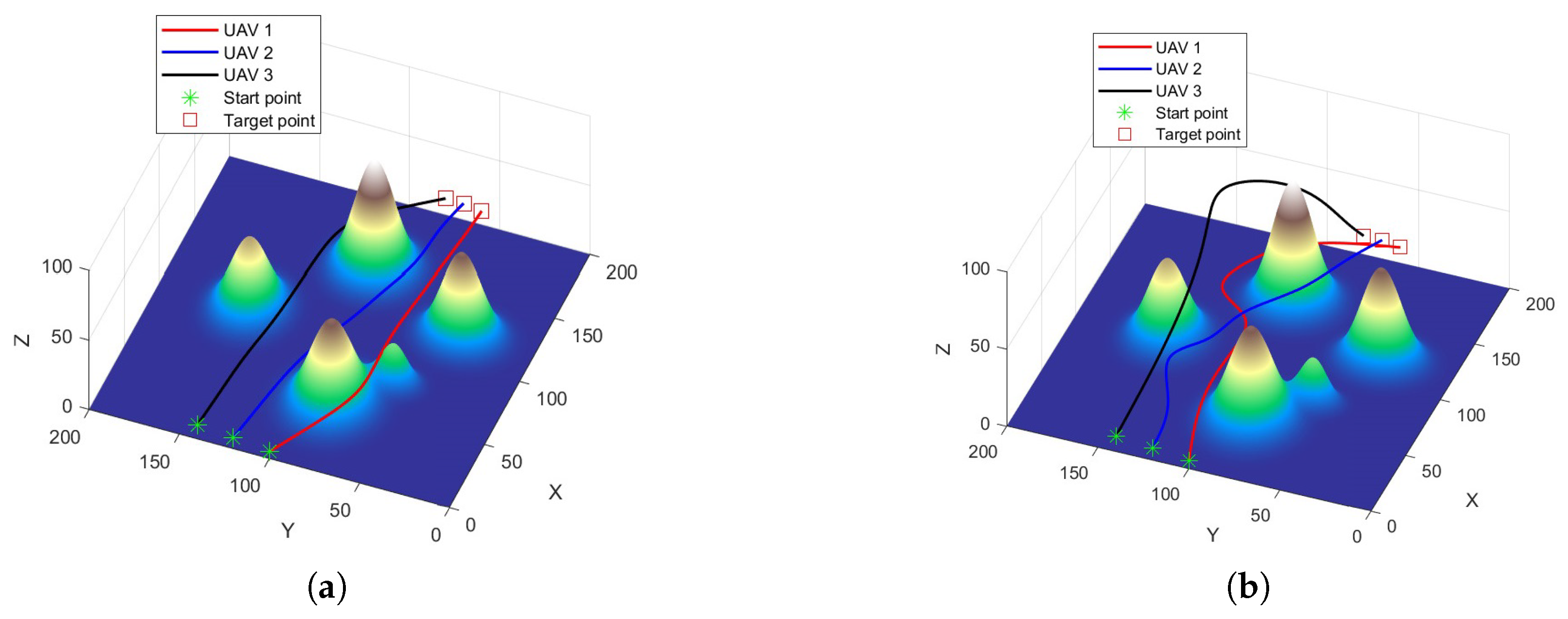
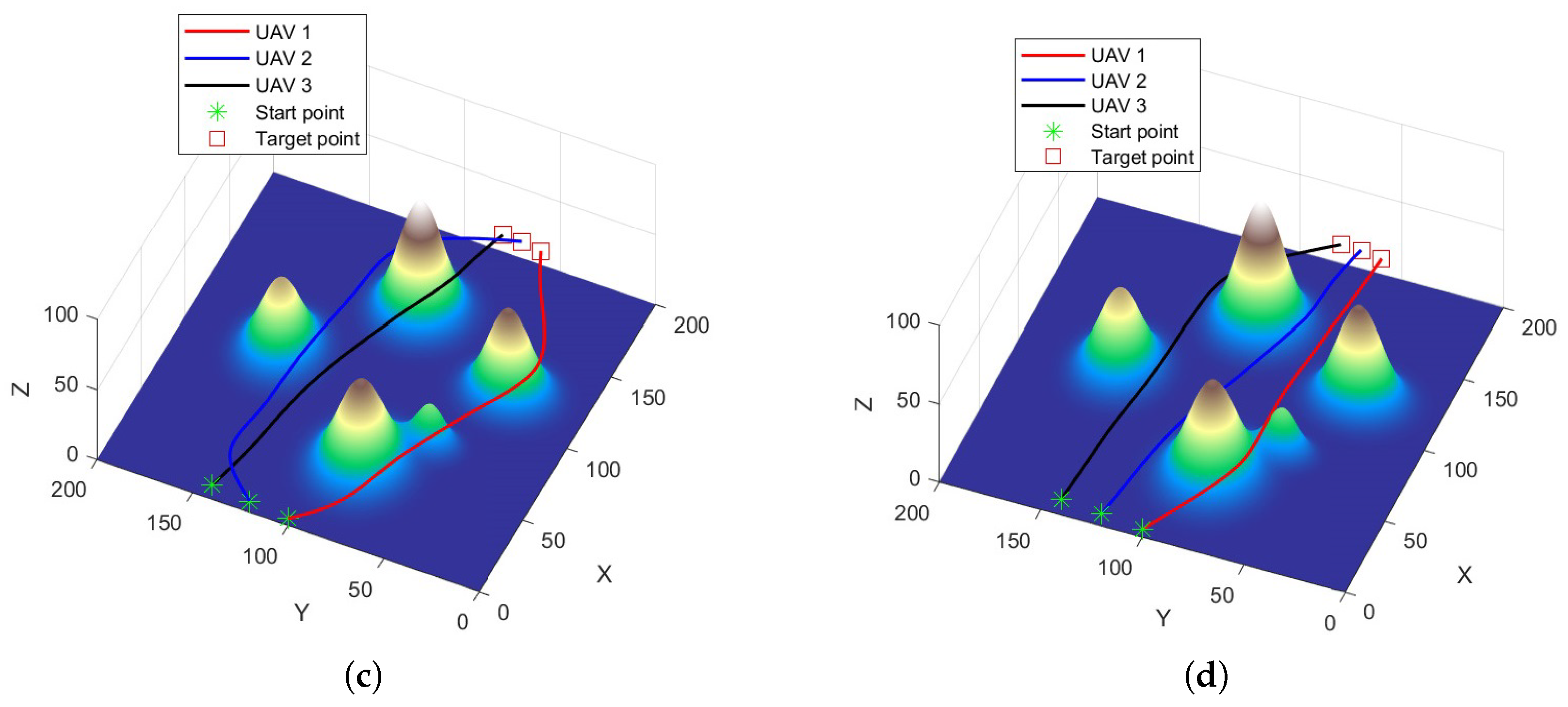
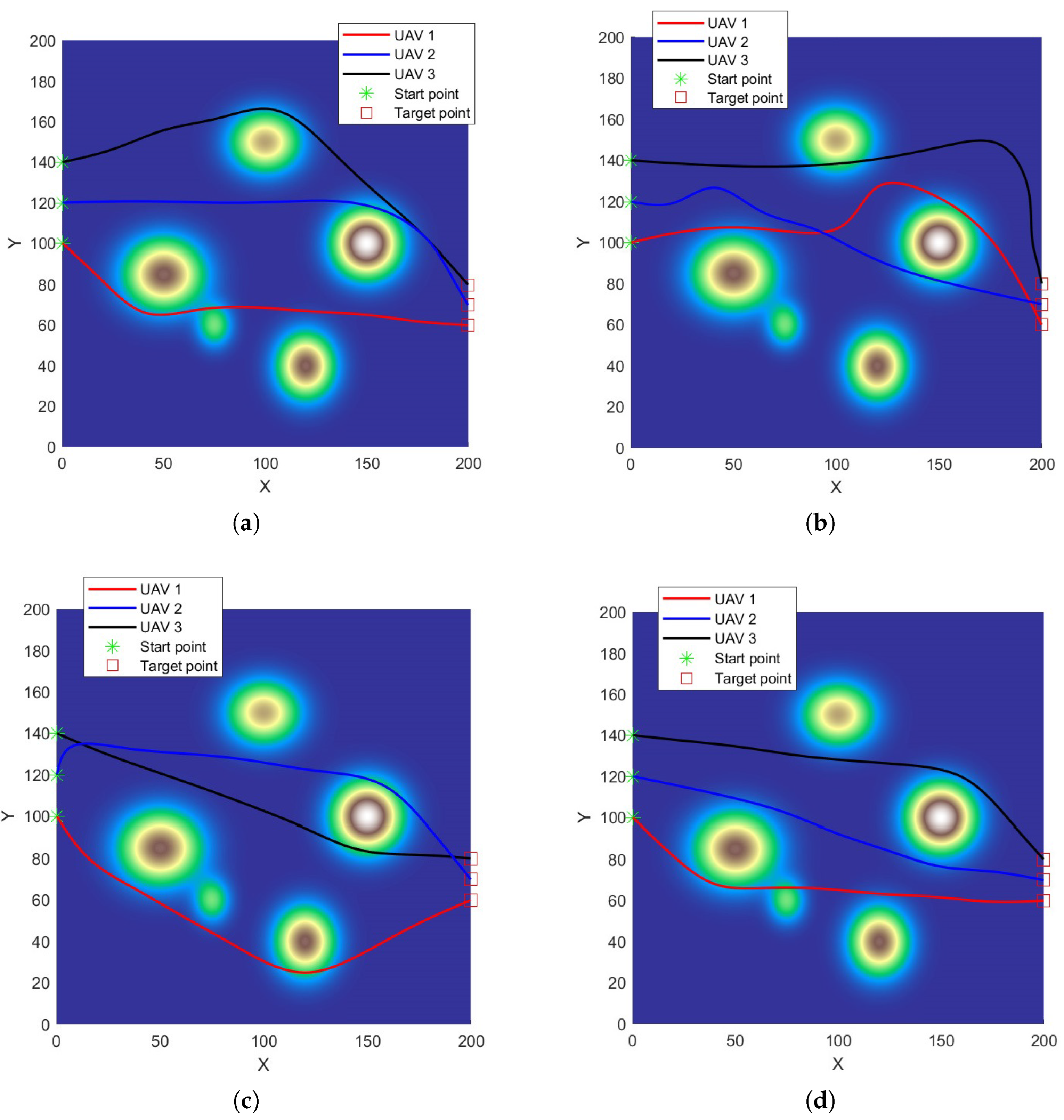
This section presents the simulation results for the threat-free environment (Scenario 1). Figure 4 and Figure 5 visually display the 3D and top views of the cooperative paths planned by the four algorithms in Scenario 1. From these figures, it is evident that while all four algorithms can generate collision-free and safe paths for multiple UAVs, significant disparities exist in the quality of the planned trajectories. Specifically, RLHSSA generates feasible and high-quality flight paths for each UAV, whereas the paths produced by MSIDE, SDPSO, and HGWODE are noticeably inferior in terms of safety and path length.
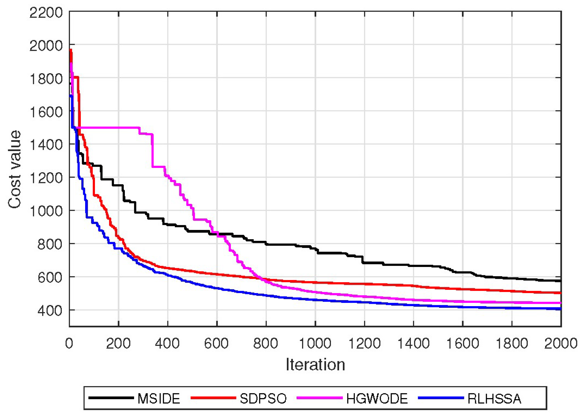
Furthermore, Figure 6 displays the convergence curves for the four algorithms in Scenario 1. This figure illustrates the correlation between the objective function value and the number of iterations, clearly showing that RLHSSA exhibits faster convergence speed and achieves a significantly lower final objective function value compared to MSIDE, SDPSO, and HGWODE. This indicates that RLHSSA is capable of efficiently finding optimal or near-optimal solutions in this scenario.
Statistical metrics from 30 independent runs in Scenario 1 are summarized in Table 6. These metrics include the minimum (Best), maximum (Worst), mean fitness (Mean), the standard deviation (Std) of the fitness values, the average computational time (Mean Time), and the success rate (SR). SR denotes the percentage of successful runs that achieve feasible and constraint-satisfying paths.
As shown in Table 6, RLHSSA consistently outperforms all comparison algorithms across the metrics of solution quality and reliability. RLHSSA achieves the lowest Best, Worst, and Mean values, highlighting its exceptional ability to find optimal solutions and avoid convergence to local optima. Furthermore, the significantly lower Std value for RLHSSA indicates its superior stability and robustness across multiple runs, suggesting that its performance is less susceptible to the stochastic nature of the optimization process. The highest SR for RLHSSA further confirms its reliability in consistently finding feasible and valid paths in the threat-free environment. Crucially, the “Mean Time (s)” metric shows that the computational times for all four algorithms are comparable. This demonstrates that RLHSSA achieves its superior performance without introducing significant computational overhead.

5.3. Simulation Results in Scenario 2

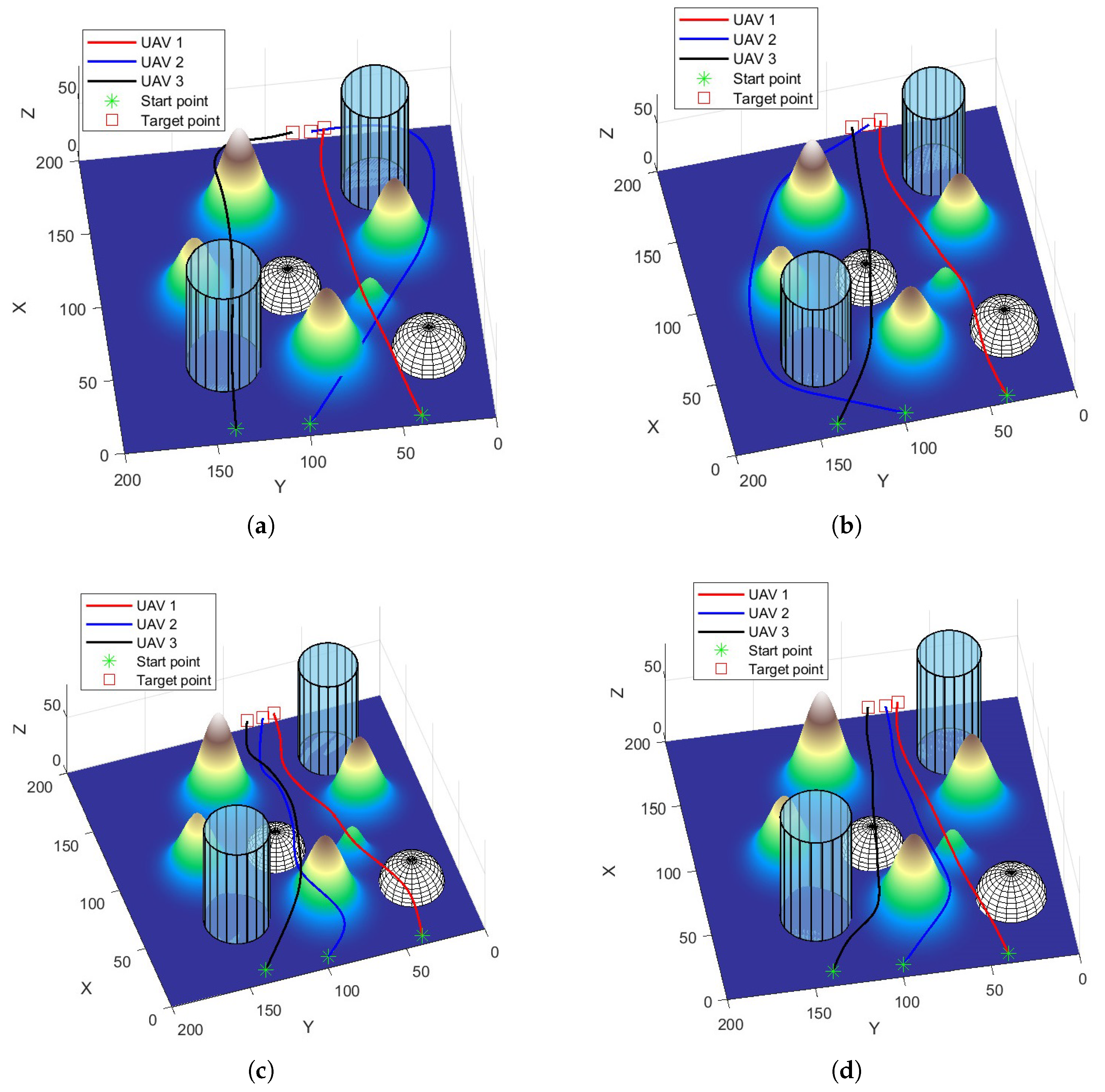
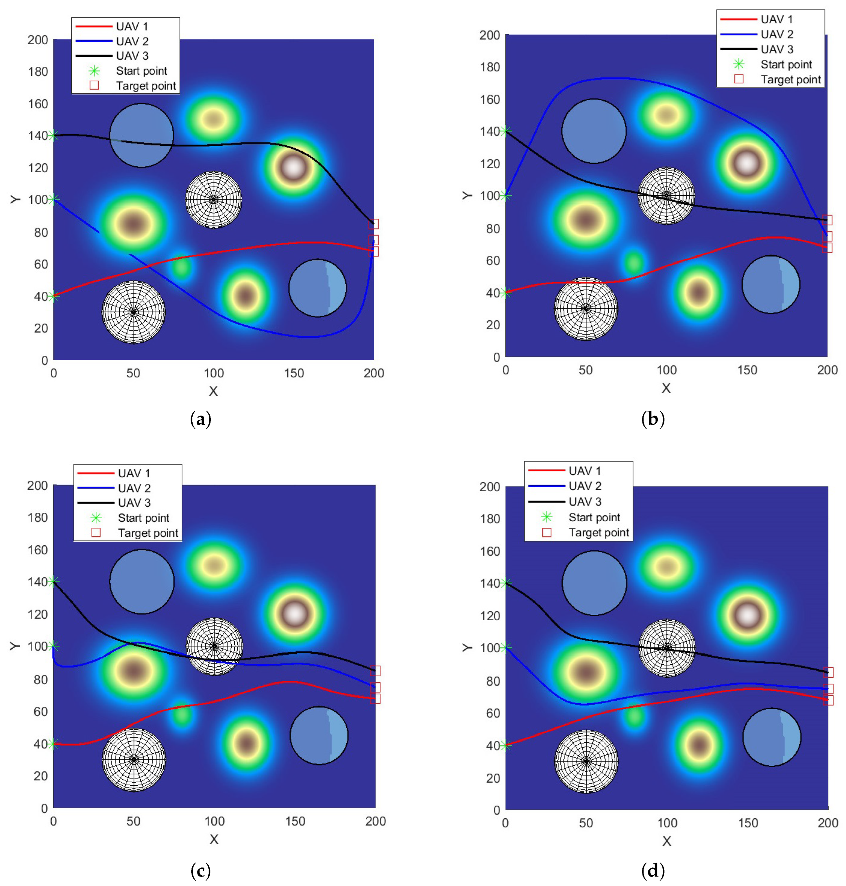
To assess the proposed algorithm’s performance under more challenging conditions, simulation experiments were conducted in the threatened environment (Scenario 2), which includes various threats and no-fly zones. Figure 7 and Figure 8 visually present the 3D and top views of the cooperative paths planned by the four algorithms in Scenario 2. Observation of these figures highlights significant differences in the quality and safety of the paths produced by the different algorithms. Under this challenging flight environment, RLHSSA demonstrates excellent performance, planning the safest and shortest flight paths for each UAV. In contrast, the other algorithms exhibit various limitations in generating optimal paths in this challenging scenario. MSIDE appears to have problems in path planning in this environment; its planned trajectories cannot guarantee the safety of each UAV passing through this area, indicating a possibility of collisions. While SDPSO and HGWODE are capable of providing safe and feasible paths, their generated trajectories are noticeably longer and less smooth compared to RLHSSA. This increased path length may lead to longer flight time and higher energy consumption.
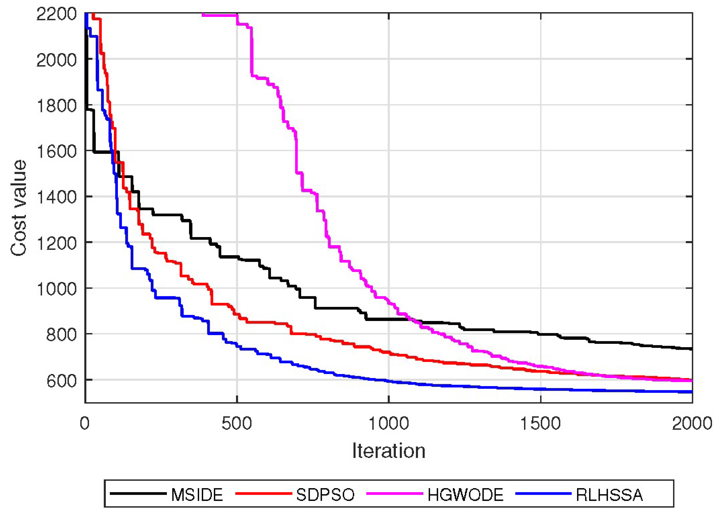
Figure 9 displays the convergence trends of the four methods in Scenario 2, illustrating their search efficiency and solution-finding capabilities. As observed from the figure, all algorithms demonstrate a decreasing trend in cost value with increasing iterations, indicating their convergence towards a solution. However, significant differences in convergence speed and final solution quality are evident among the algorithms. The proposed RLHSSA algorithm exhibits the fastest convergence rate, achieving the lowest cost value within 2000 iterations, which highlights its superior search efficiency and global optimization capability in this complex scenario.
Table 7 summarizes the statistical outcomes of the four algorithms after 30 runs in Scenario 2, demonstrating that the proposed RLHSSA algorithm consistently achieves the best performance across all indicators. It records the lowest mean objective value of 581.4147, demonstrating its superior ability to find high-quality solutions. Furthermore, with a low standard deviation of 8.4732 and a 100% success rate, RLHSSA exhibits remarkable stability and robustness in navigating the complex and constrained environment. Crucially, the “Mean Time (s)” metric again shows that the computational times for all algorithms are comparable. This confirms that the superior performance of RLHSSA is achieved without imposing any significant computational penalty, even in this more complex threatened environment.

6. Conclusions

This study addresses the intricate challenge of cooperative route planning for multiple UAVs operating in mountainous regions, with particular attention to threat presence. To solve this challenge, we propose a path planning approach that employs the RLHSSA, a novel hybrid optimization algorithm. It facilitates the generation of optimal, safe, and efficient flight paths while effectively avoiding terrain obstacles. The proposed RLHSSA integrates three distinct optimization operators: the Elite Sparrow Search Algorithm (Elite-SSA) for refined exploitation, alongside the Adaptive Differential Perturbation and Adaptive Levy Flight strategies for robust exploration. A key innovation is the use of a Reinforcement Learning (RL) agent that dynamically schedules these operators, ensuring an intelligent balance between search breadth and depth to effectively prevent premature convergence.
Subsequently, simulation experiments were conducted in two different three-dimensional mountainous environments, comparing and evaluating the RLHSSA algorithm with three advanced methods. The experimental findings consistently indicate the superiority of RLHSSA over other methods regarding solution accuracy, convergence speed, and stability. This validates the utility of RLHSSA for cooperative path planning of multi-UAVs in mountainous environments.
Future work will focus on applying the algorithm to dynamic scenarios characterized by stochastic threats. Furthermore, the transferability of the RLHSSA framework to other multi-agent systems and complex optimization problems will be further investigated.

Author Contributions

Conceptualization, L.L.; methodology, W.S. and W.J.; software, L.L. and R.H.; validation, L.L. and W.S.; formal analysis, W.J.; investigation, L.L.; resources, W.S.; data curation, W.S. and R.H.; writing—original draft preparation, L.L.; writing—review and editing, L.L. and W.S.; visualization, W.S. All authors have read and agreed to the published version of the manuscript.

Funding

This research was funded by the National Natural Science Foundation of China (No. 62371375), the Shaanxi Key R&D Plan Key Industry Innovation Chain Project, the Shaanxi “Hundred Teams” Project for University-Enterprise Collaboration 2025, and the Xi’an Science and Technology Plan Project (No. 2025JH-KXGC-0007).

Data Availability Statement

The raw data supporting the conclusions of this article will be made available by the authors upon request.

Conflicts of Interest

Author Wei Jia was employed by the company Xi’an ASN Technology Group Co., Ltd. The remaining authors declare that the research was conducted in the absence of any commercial or financial relationships that could be construed as a potential conflict of interest.

References

  1. Skorobogatov, G.; Barrado, C.; Salamí, E. Multiple UAV systems: A survey. Unmanned Syst. 2020, 8, 149–169. [Google Scholar] [CrossRef]
  2. Erdelj, M.; Natalizio, E.; Chowdhury, K.R.; Akyildiz, I.F. Help from the sky: Leveraging UAVs for disaster management. IEEE Pervas. Comput. 2017, 16, 24–32. [Google Scholar] [CrossRef]
  3. Wang, K.; Yang, P.; Lv, W.S.; Zhu, L.Y.; Yu, G.M. Current status and development trend of UAV remote sensing applications in the mining industry. Chin. J. Eng. 2020, 42, 1085–1095. [Google Scholar]
  4. Zhou, X.Y.; Jia, W.; He, R.F.; Sun, W. High-Precision localization tracking and motion state estimation of ground-based moving target utilizing unmanned aerial vehicle high-altitude reconnaissance. Remote Sens. 2025, 17, 735. [Google Scholar] [CrossRef]
  5. Hong, Y.; Kim, S.; Kwon, Y.; Choi, S.; Cha, J. Safe and Efficient Exploration Path Planning for Unmanned Aerial Vehicle in Forest Environments. Aerospace 2024, 11, 598. [Google Scholar] [CrossRef]
  6. Yu, X.; Luo, W. Reinforcement learning-based multi-strategy cuckoo search algorithm for 3D UAV path planning. Expert Syst. Appl. 2023, 223, 119910. [Google Scholar] [CrossRef]
  7. Qadir, Z.; Zafar, M.H.; Moosavi, S.K.R.; Le, K.N.; Mahmud, M.A.P. Autonomous UAV path-planning optimization using metaheuristic approach for predisaster assessment. IEEE Internet Things 2021, 9, 12505–12514. [Google Scholar] [CrossRef]
  8. Abdel-Basset, M.; Mohamed, R.; Sallam, K.M.; Hezam, I.M.; Munasinghe, K.; Jamalipour, A. A multiobjective optimization algorithm for safety and optimality of 3-D route planning in UAV. IEEE Trans. Aerosp. Electron. Syst. 2024, 60, 3067–3080. [Google Scholar] [CrossRef]
  9. Chen, J.; Zhang, R.; Zhao, H.; Li, J.; He, J. Path planning of multiple unmanned aerial vehicles covering multiple regions based on minimum consumption ratio. Aerospace 2023, 10, 93. [Google Scholar] [CrossRef]
  10. Zhang, Z.; Zhu, L. A Review on Unmanned Aerial Vehicle Remote Sensing: Platforms, Sensors, Data Processing Methods, and Applications. Drones 2023, 7, 398. [Google Scholar] [CrossRef]
  11. He, W.J.; Qi, X.G.; Liu, L.F. A novel hybrid particle swarm optimization for multi-UAV cooperate path planning. Appl. Intell. 2021, 51, 7350–7364. [Google Scholar] [CrossRef]
  12. Xu, L.; Cao, X.B.; Du, W.B.; Li, Y.M. Cooperative path planning optimization for multiple UAVs with communication constraints. Knowl.-Based Syst. 2023, 260, 110164. [Google Scholar] [CrossRef]
  13. Pan, Z.; Zhang, C.; Xia, Y.; Xiong, H.; Shao, X. An improved artificial potential field method for path planning and formation control of the multi-UAV systems. IEEE T Circuits-II 2021, 69, 1129–1133. [Google Scholar] [CrossRef]
  14. Wang, W.T.; Li, X.L.; Tian, J. UAV formation path planning for mountainous forest terrain utilizing an artificial rabbit optimizer incorporating reinforcement learning and thermal conduction search strategies. Adv. Eng. Inform. 2024, 62, 102947. [Google Scholar] [CrossRef]
  15. Sun, B.; Niu, N. Multi-AUVs cooperative path planning in 3D underwater terrain and vortex environments based on improved multi-objective particle swarm optimization algorithm. Ocean Eng. 2024, 311, 118944. [Google Scholar] [CrossRef]
  16. Xu, C.; Xu, M.; Yin, C. Optimized multi-UAV cooperative path planning under the complex confrontation environment. Comput. Commun. 2020, 162, 196–203. [Google Scholar] [CrossRef]
  17. Li, Y.; Dong, X.; Ding, Q.; Xiong, Y.; Wang, T. Improved A-STAR algorithm for power line inspection UAV path planning. Energies 2024, 17, 5364. [Google Scholar] [CrossRef]
  18. Wang, J.; Li, Y.; Li, R.; Chen, H.; Chu, K. Trajectory planning for UAV navigation in dynamic environments with matrix alignment Dijkstra. Soft Comput. 2022, 26, 12599–12610. [Google Scholar] [CrossRef]
  19. Guo, Y.; Liu, X.; Jiang, W.; Zhang, W. HDP-TSRRT*: A time-space cooperative path planning algorithm for multiple UAVs. Drones 2023, 7, 170. [Google Scholar] [CrossRef]
  20. Zhang, Z.; Li, J.; Wang, J. Sequential convex programming for nonlinear optimal control problems in UAV path planning. Aerosp. Sci. Technol. 2018, 76, 280–290. [Google Scholar] [CrossRef]
  21. Wu, Y.; Liang, T.; Gou, J.; Tao, C.; Wang, H. Heterogeneous mission planning for multiple UAV formations via metaheuristic algorithms. IEEE Trans. Aerosp. Electron. Syst. 2023, 59, 3924–3940. [Google Scholar] [CrossRef]
  22. Gupta, H.; Verma, O.P. A novel hybrid coyote-particle swarm optimization algorithm for three-dimensional constrained trajectory planning of unmanned aerial vehicle. Appl. Soft Comput. 2023, 147, 110776. [Google Scholar] [CrossRef]
  23. Ab Wahab, M.N.; Nazir, A.; Khalil, A.; Ho, W.J.; Akbar, M.F.; Noor, M.H.M.; Mohamed, A.S.A. Improved genetic algorithm for mobile robot path planning in static environments. Expert Syst. Appl. 2024, 249, 123762. [Google Scholar] [CrossRef]
  24. Li, X.; Yu, S. Three-dimensional path planning for AUVs in ocean currents environment based on an improved compression factor particle swarm optimization algorithm. Ocean Eng. 2023, 280, 114610. [Google Scholar] [CrossRef]
  25. Wang, Z.; Dai, D.; Zeng, Z.; He, D.; Chan, S. Multi-strategy enhanced Grey Wolf Optimizer for global optimization and real world problems. Cluster Comput. 2024, 27, 10671–10715. [Google Scholar] [CrossRef]
  26. Zhang, M.H.; Han, Y.H.; Chen, S.Y.; Liu, M.X.; He, Z.L.; Pan, N. A multi-strategy improved differential evolution algorithm for UAV 3D trajectory planning in complex mountainous environments. Eng. Appl. Artif. Intel. 2023, 125, 106672. [Google Scholar] [CrossRef]
  27. Meng, K.; Chen, C.; Wu, T.; Xin, B.; Liang, M.; Deng, F. Evolutionary state estimation-based multi-strategy jellyfish search algorithm for multi-UAV cooperative path planning. IEEE Trans. Intell. Veh. 2024, 10, 2490–2507. [Google Scholar] [CrossRef]
  28. Wang, F.; Wang, X.; Sun, S. A reinforcement learning level-based particle swarm optimization algorithm for large-scale optimization. Inform. Sci. 2022, 602, 298–312. [Google Scholar] [CrossRef]
  29. Zhang, S.; Li, Y.; Dong, Q. Autonomous navigation of UAV in multi-obstacle environments based on a deep reinforcement learning approach. Appl. Soft Comput. 2022, 115, 108194. [Google Scholar] [CrossRef]
  30. Skarka, W.; Ashfaq, R. Hybrid machine learning and reinforcement learning framework for adaptive UAV obstacle avoidance. Aerospace 2024, 11, 870. [Google Scholar] [CrossRef]
  31. Niu, Y.; Yan, X.; Wang, Y.; Niu, Y. Three-dimensional collaborative path planning for multiple UCAVs based on improved artificial ecosystem optimizer and reinforcement learning. Knowl.-Based Syst. 2023, 276, 110782. [Google Scholar] [CrossRef]
  32. Qu, C.; Gai, W.; Zhong, M.; Zhang, J. A novel reinforcement learning based grey wolf optimizer algorithm for unmanned aerial vehicles (UAVs) path planning. Appl. Soft Comput. 2020, 89, 106099. [Google Scholar] [CrossRef]
  33. Jiaqi, S.; Li, T.; Hongtao, Z.; Xiaofeng, L.; Tianying, X. Adaptive multi-UAV path planning method based on improved gray wolf algorithm. Comput. Electr. Eng. 2022, 104, 108377. [Google Scholar] [CrossRef]
  34. Xue, J.K.; Shen, B. A novel swarm intelligence optimization approach: Sparrow search algorithm. Syst. Sci. Control Eng. 2020, 8, 22–34. [Google Scholar] [CrossRef]
  35. Niu, Y.B.; Yan, X.; Wang, Y.; Niu, Y.Z. Three-dimensional UCAV path planning using a novel modified artificial ecosystem optimizer. Expert Syst. Appl. 2023, 217, 119499. [Google Scholar] [CrossRef]
  36. Lv, L.; Liu, H.J.; He, R.; Jia, W.; Sun, W. A Novel HGW Optimizer with Enhanced Differential Perturbation for Efficient 3D UAV Path Planning. Drones 2025, 9, 212. [Google Scholar] [CrossRef]
  37. Gharehchopogh, F.S.; Namazi, M.; Ebrahimi, L.; Abdollahzadeh, B. Advances in sparrow search algorithm: A comprehensive survey. Arch. Comput. Method. E. 2023, 30, 427–455. [Google Scholar] [CrossRef]
  38. He, Y.; Wang, M. An improved chaos sparrow search algorithm for UAV path planning. Sci. Rep. 2024, 14, 366. [Google Scholar] [CrossRef]
  39. Amirsadri, S.; Mousavirad, S.J.; Ebrahimpour-Komleh, H. A Levy flight-based grey wolf optimizer combined with back-propagation algorithm for neural network training. Neural Comput. Appl. 2018, 30, 3707–3720. [Google Scholar] [CrossRef]
  40. Gong, G.M.; Fu, S.W.; Huang, H.S.; Huang, H.F.; Luo, X. Multi-strategy improved snake optimizer based on adaptive lévy flight and dual-lens fusion. Cluster Comput. 2025, 28, 268. [Google Scholar] [CrossRef]
  41. Liu, H.; Zhang, X.; Zhang, H.; Li, C.; Chen, Z. A reinforcement learning-based hybrid Aquila Optimizer and improved Arithmetic Optimization Algorithm for global optimization. Expert Syst. Appl. 2023, 224, 119898. [Google Scholar] [CrossRef]
  42. Yu, Z.H.; Si, Z.J.; Li, X.B.; Wang, D.; Song, H.B. A novel hybrid particle swarm optimization algorithm for path planning of UAVs. IEEE Internet Things 2022, 9, 22547–22558. [Google Scholar] [CrossRef]
  43. Yu, X.B.; Jiang, N.J.; Wang, X.M.; Li, M.Y. A hybrid algorithm based on grey wolf optimizer and differential evolution for UAV path planning. Expert Syst. Appl. 2023, 215, 119327. [Google Scholar] [CrossRef]
  44. Qu, C.; Gai, W.; Zhang, J.; Zhong, M. A novel hybrid grey wolf optimizer algorithm for unmanned aerial vehicle (UAV) path planning. Knowl.-Based Syst. 2020, 194, 105530. [Google Scholar] [CrossRef]
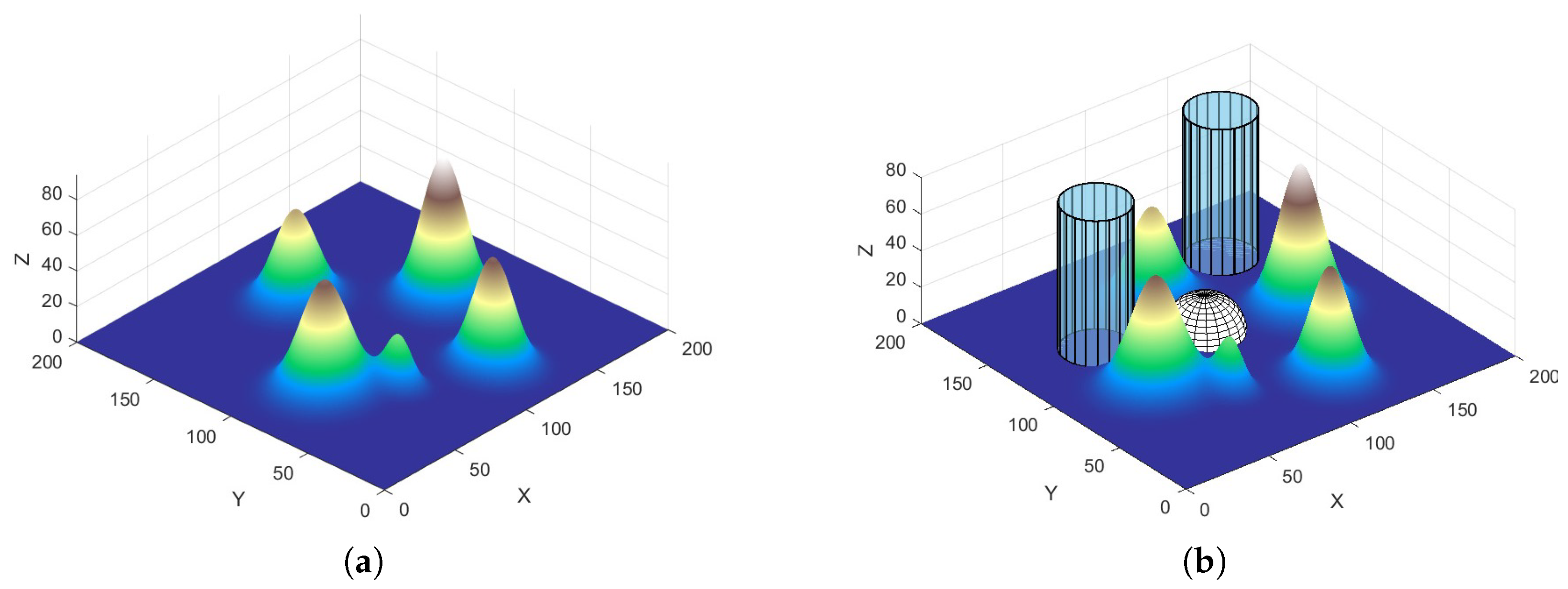
Figure 1. Environmental model. (a) Mountain obstacles. (b) Obstacle terrain.
Aerospace 12 01025 g001
Figure 2. Diagram of UAV flight attitude and path segments.
Aerospace 12 01025 g002
Figure 3. Computation of threat cost.
Aerospace 12 01025 g003
Figure 4. 3D flight paths visualization of three UAVs in Scenario 1: (a) MSIDE; (b) SDPSO; (c) HGWODE; (d) RLHSSA.
Aerospace 12 01025 g004aAerospace 12 01025 g004b
Figure 5. Three UAVs flight trajectories (top view) in Scenario 1: (a) MSIDE; (b) SDPSO; (c) HGWODE; (d) RLHSSA.
Aerospace 12 01025 g005
Figure 6. Convergence curves of four algorithms in Scenario 1.
Aerospace 12 01025 g006
Figure 7. Three-dimensional flight path visualization of three UAVs in Scenario 2: (a) MSIDE; (b) SDPSO; (c) HGWODE; (d) RLHSSA.
Aerospace 12 01025 g007
Figure 8. Three UAVs’ flight trajectories (top view) in Scenario 2: (a) MSIDE; (b) SDPSO; (c) HGWODE; (d) RLHSSA.
Aerospace 12 01025 g008
Figure 9. Convergence curves of four algorithms in Scenario 2.
Aerospace 12 01025 g009
Table 1. The Q-table framework for strategy scheduling.
StateAction
a 1 : Elite-SSA a 2 : Diff. Perturbation a 3 : Levy Flight
s 1 Q ( s 1 , a 1 ) Q ( s 1 , a 2 ) Q ( s 1 , a 3 )
s 2 Q ( s 2 , a 1 ) Q ( s 2 , a 2 ) Q ( s 2 , a 3 )
s 10 Q ( s 10 , a 1 ) Q ( s 10 , a 2 ) Q ( s 10 , a 3 )
Table 2. Parameters of multiple UAVs.
UAV No.Start PointTarget Point
Scenario 11(0, 100, 5)(200, 60, 10)
2(0, 120, 8)(200, 70, 12)
3(0, 140, 10)(200, 80, 12)
Scenario 21(0, 40, 8)(200, 68, 8)
2(0, 100, 10)(200, 75, 6)
3(0, 140, 12)(200, 85, 7)
Table 3. Information of threat and NFZs in Scenario 2.
Threat/NFZThreat/NFZ CenterRadiusHeightThreat Level
Threat(50, 30, 0)2010
Threat(100, 100, 0)1810
NFZ(55, 140)2080
NFZ(165, 45)1880
Table 4. Algorithm parameter setting.
AlgorithmParameter
MSIDE F min = 0 , F max = 1 , C R = 0.8
SDPSO w : 0.4 0.9 , c 1 = c 2 : 0.4 2.0
HGWODE a = 2 0 , C r = 0.5
RLHSSA S T = 0.8 , μ = 0.5 , λ = 1.5,
Table 5. Parameter definitions and values.
ParameterDescriptionValue
t max Maximum iteration count2000
N P Population count50
Mwaypoint count7
[ H min , H max ] UAV operational altitude range[1, 100]
ϑ max Max turning angle 30
ξ max Max climbing angle 30
h s a f e safe-altitude threshold15
D s a f e Inter-UAV safe distance20
Table 6. Experimental outcomes in Scenario 1 across 30 independent runs.
NO.IndicatorsMSIDESDPSOHGWODERLHSSA
1Best430.0323410.2035405.4126396.3353
2Worst586.0367485.3387472.5805416.0802
3Mean468.7183434.4157426.9850405.0570
4Std43.111416.751912.40364.0826
5SR (%)70.083.3390.0100.0
6 Mean Time ( s ) 12.4811.8713.3212.81
Table 7. Experimental outcomes in Scenario 2 across 30 independent runs.
NO.IndicatorsMSIDESDPSOHGWODERLHSSA
1Best625.3503583.6828585.7339570.1830
2Worst920.1053832.2043803.0355609.9120
3Mean737.2827648.8387625.1940581.4147
4Std87.802762.776848.38408.4732
5SR (%)60.076.6786.67100.0
6 Mean Time ( s ) 15.3813.8315.7414.28
Disclaimer/Publisher’s Note: The statements, opinions and data contained in all publications are solely those of the individual author(s) and contributor(s) and not of MDPI and/or the editor(s). MDPI and/or the editor(s) disclaim responsibility for any injury to people or property resulting from any ideas, methods, instructions or products referred to in the content.