High-Resolution CAD-Based Shape Parametrisation of a U-Bend Channel

Abstract

The parametrisation of the geometry in shape optimisation has an important influence on the quality of the optimum and the rate of convergence of the optimiser. Refinement studies for the parametrisation are not shown in the literature, as most methods use non-orthogonal parametrisations, which cause issues with convergence when the parametrisation is refined. The NURBS-based parametrisation with complex constraints (NSPCC) is the only CAD-based parametrisation method that guarantees orthogonal shape modes by constructing an optimal basis. We conduct a parametrisation refinement study for the benchmark turbomachinery cooling bend (U-bend) geometry, an intially symmetric geometry. Using an adjoint RANS solver, we optimise for mininmal total pressure drop. The results show significant effects of the control net density on the final shape, with the finest control net producing an asymmetric optimal shape resembling strakes that induces swirl ahead of the bend. These asymmetric modes have not been reported in the literature so far. We also demonstrate that the convergence rate of the optimiser is not significantly affected by the refinement of the parametrisation. The effectiveness of these shape features obtained with single-point optimisation is evaluated for a range of Reynolds numbers. It is shown that total pressure drop reduction is not sensitive to Reynolds number.

1. Introduction

Shape optimisation of aircraft wings, turbomachinery blades, or automotive ducts has become a widely used technique over recent decades. While early studies in shape optimisation used gradient-free approaches, more recent work in the past decade has firmly established gradient-based approaches as the method of choice given their superior efficiency for the large number of design variables that are often required [1]. This implies, however, that gradients are also computed for the shape parametrisation. Using the adjoint approach to compute the gradient of an objective to be minimised with respect to the design variables makes the cost of gradient computation independent of the size of the design space and allows for consideration of a much wider range of parametrisations for the design. At the very rich end of the spectrum, node-based methods consider the displacement of every surface grid node as a design variable [2,3,4,5], using the richest design space the computational method can possibly treat. This design space contains unwanted oscillatory modes which need to be regularised. There is no analysis in the literature of how to control this regularisation to appropriately distinguish between unwanted and desirable high-wavenumber modes. A more rigorous approach is the CAD-based NSPCC method, which defines the possible shape modes in CAD rather than on the mesh, and hence does not need regularisation. This is the approach employed in this work.

A widely studied optimisation benchmark testcase is the flow in serpentine cooling channels for turbomachinery blades. Covering the area to be cooled requires routing the channel with a number of 180${}^{\circ }$ turns, commonly referred to as ‘U-bends’, which impose high total pressure losses on the coolant flow, and hence impair engine efficiency. The testcase we consider in this paper is the VKI U-bend benchmark case [6,7], shown in Figure 1, which has seen experimental validation for both the baseline and an optimised shape. The benchmark case allows for modifications to the bend section in order to minimise mass-averaged pressure loss. The Boundary Representation (BRep) of the U-bend geometry along with some of the geometric constraints is shown in Figure 1 and the design patches considered in this study are highlighted in green. The BRep of the baseline geometry consists of twelve NURBS patches: four planar rectangular patches that form the inlet and outlet channels, as well as four curved patches that form the U-bend. $G_2$ continuity (continuous curvature, zero in this case) is enforced at the upstream and downstream ends of the deformable part. $G_1$ continuity is imposed at all ‘cross-sectional’ patch interfaces, i.e., those that run mostly perpendicular to the flow between the originally planar and curved patches. $G_0$ continuity is imposed on the remaining patch interfaces that align with the flow, i.e., interfaces between originally planar patches and originally curved patches.

Figure 1. Baseline U-bend geometry with design patches highlighted in green and geometric constraints imposed on different edges.

Earlier experimental validation of CFD results of both baseline and optimal geometries [6,8] found significant discrepancies, as RANS-based simulations were unable to accurately capture secondary flow effects, streamline curvature and flow separation. More recently, Alessi et al. [9] computed U-bend flow characteristics using the Large Eddy Simulation (LES) approach and compared with RANS-based simulation. They observed that the LES model could accurately predict the complex vortex structures and flow separation associated with the U-bend geometry. However major flow trends were well captured using a RANS-based solver. Hence, RANS-based shape optimisation can be considered to be suitable for the U-bend geometry. Furthermore, we note that LES-based optimisation is not feasible for routine application due to (a) its computational cost, but also (b) due to the fact that no adjoints exist for LES models, which resolve the chaotic nature of the flow, as this implies blow-up of the adjoint sensitivities. The use of adjoints to compute sensitivities is essential, as this is the only known way to compute them at constant cost. Alternatives, such as finite differences, forward-mode automatic differentiation or the complex variable method have a cost that scales linearly with the number of design variables, which is prohibitive for highly refined design spaces.

The performance of shape optimisation is critically dependent on the design modes including the relevant shape modes to control the flow. Since those “flow” modes are not known a priori, design spaces need to be rich enough to include the widest range of possible modes. In nearly all parametrisation methods in the literature, smoothness of the shape is achieved by modes that are either smooth by construction, such as Radial Basis Functions (RBFs) [10], or are smoothened by built-in regularisation, e.g., in node-based methods [2,3,4,5]. Convergence of linear systems strongly depends on the diagonal dominance of its Jacobian matrix; however, the global support of RBF or the large stencil of regularised methods produce non-sparse ill-conditioned Jacobians, which result in poor convergence toward the optimum.

The NURBS-based parametrisation with complex constraints (NSPCC) method derives orthogonal shape modes directly from the BRep of a CAD model using singular value decomposition (SVD). This derives an optimal orthogonal basis for the shape modes, which is a crucial ingredient to obtain a convergence rate independent of the number of design variables. Hence, NSPCC is used in this work.

In contrast to earlier works on NSPCC, the NSPCC geometry kernel is differentiated using source transformation algorithmic differentiation in adjoint mode. This approach enables the efficient reverse-mode, or adjoint differentiation of the entire design chain, including CFD, meshing, and CAD operations, in a single ‘one-shot’ computation. Consequently, gradient computation remains independent of the size of the control net density. To investigate the impact of control net distribution on shape optimisation, we perform shape optimisation using three different levels of control net distribution with the VKI U-bend benchmark test case. Our objective is to evaluate how variations in control net density affect optimisation convergence, the ability to capture fine geometric details, and the trade-off between computational complexity and efficiency.

The paper is organised as follows. Section 2 gives a brief review of the key parametrisation approaches applied to the U-bend benchmark case. Section 3 presents the NURBS-based parametrisation with complex constraints (NSPCC) method considered in this study. Section 4 discusses the reverse differentiation of the entire design chain and its assembly for shape optimisation. One-shot aerodynamic shape optimisation of an internal turbine cooling channel including flow solver validation, mesh convergence study, and CAD sensitivity verification is discussed in Section 5. In Section 6, the influence of shape parametrisation is presented with an analysis of the results of the optimisation and the effectiveness of the methodology. Conclusions and future work are presented in Section 7.

2. Shape Parametrisation Approaches

2.1. Gradient-Free Approaches

Earlier applications of shape optimisation mainly used gradient-free optimisation methods, which scale poorly with the number of design variables. Therefore, parametrisations were typically chosen to limit the number of design variables. The original work on the U-bend by Verstraete et al. [7] considered only 2D changes in the plane perpendicular to the bend. They parametrised the ${180}^{\circ }$ bend region using piecewise Bézier curves and considered their control points as design variables. The authors used a metamodel-assisted differential evolution algorithm; CFD results for baseline and 2D optimised geometry can be found in [6]. Namgoong et al. [8] performed both 2D and 3D CAD-based shape optimisation using design of experiments and a surrogate design space model. To reduce computational complexity, only the inner U-bend surface was considered for optimisation. This region is parametrised using spline curves, with control points allowed to deform symmetrically. Kiyici et al. [10] employed an RBF-based mesh morphing approach to deform the U-bend region, aiming to minimise pressure loss and enhance heat transfer performance. They utilised a metamodel-assisted evolutionary algorithm and incorporated ten ribs before and after the U-turn, excluding the bend region.

2.2. Gradient-Based Approaches

The availability of gradients allows for considering a much larger design space. Willeke et al. [11] consider 2D displacements of boundary grid points as design variables and use a continuous adjoint approach to compute the derivatives. However, only a 2D variation of the shape is considered, which offers limited ability to minimise secondary flow effects but instead focuses on pressure loss reduction by suppressing flow separation along the internal side of the bend. He et al. [12] also consider the U-bend and use Free-Form Deformation (FFD) with 63 FFD points that are allowed to move in the z or $x,y$ directions, resulting in 113 design variables. Verstraete et al. [13] parametrised the U-bend region with trivariate B-spline volumes with external control points as design variables, resulting in 540 degrees of freedom. Kim et al. [14] employed topology optimisation to minimise pressure loss in the U-bend region. Recently, Alessi et al. [15] utilised Large Eddy Simulation (LES) in an optimisation framework, deforming each design surface grid point in the direction normal to the surface while freezing the deformation in the z direction, thereby restricting the design space.

2.3. CAD-Free vs. CAD-Based Parametrisation Approaches

A common feature of the aforementioned approaches is that they are ‘CAD-free’; while the baseline shape is derived from a CAD model, this model is not included in the optimisation loop and hence not updated. The resulting optimal shape is not in a CAD format and a ‘return to CAD’ step needs to be added to make this shape available for further design, analysis or manufacturing. This step typically requires approximation of the optimised shape using a given or adapted CAD topology, and relevant features of the optimal shape may be lost. On the other hand, CAD-based parametrisation approaches use a CAD model in the design loop, hence updating both the CAD model and the corresponding computational mesh consistently within the design loop. Feature-based parametric CAD systems, such as CATIA, SolidWorks, and OpenCASCADE, create geometry by defining, combining and evolving features, with the construction history recorded in the ‘feature-tree’. Parameters embedded in the feature tree can serve as design variables and be updated by the optimiser, thus producing the optimal model in CAD at the end of the design loop. Therefore, CAD-based methods can be integrated seamlessly with black box CFD solvers and meta-model-assisted gradient-free optimisation methods [8].

To integrate a CAD model into a gradient-based optimisation design loop, the derivative $\left({\displaystyle \frac{\mathsf{\partial }{X}_S}{\mathsf{\partial }\alpha }}\right)$ of surface grid point coordinates $\left(X_S\right)$ with respect to design variables $\left(\alpha \right)$, termed ‘shape sensitivities’, need to be obtained by differentiating the CAD model. The available options are (1) applying finite differences directly to the CAD model, (2) formulating analytic derivatives, and (3) applying algorithmic differentiation to the source code. Finite difference approaches compute the shape sensitivities by perturbing each parameter, which requires selecting an appropriate perturbation size to balance truncation and round-off errors. However, finite-size perturbations may lead to topological changes in the CAD geometry, resulting in a non-differentiable function. This can be mitigated by computing the perturbed point location on a projected surrogate surface [16,17], which may incur further approximation errors in regions of high curvature. Techniques based on analytic derivatives propose to formulate analytic derivatives for each operation in the model feature tree and concatenate these derivatives using the chain rule of calculus. Dannenhoffer et al. [18] used the open-source Constructive Solid Modeler (OpenCSM) and applied analytic differentiation to basic primitives such as circles and cylinders. However, for operations such as fillets and chamfers, direct analytic differentiation is not available, necessitating the use of finite differences for these cases. Complex feature trees with Boolean operations could then result in topological changes, giving rise to similar issues as in the full finite difference approach.

If the source code of the CAD kernel is available, such as in in-house CAD modellers or in the case of open-source CAD engine OpenCASCADE (OCCT), shape sensitivities can be obtained by applying Algorithmic Differentiation (AD) Software tools to the complete the CAD kernel. The OpenCASCADE CAD kernel has been differentiated [19,20,21] using the operator-overloading AD tool ADOL-C. While their work demonstrates reverse-mode sensitivities for smaller models, in most cases, they use the forward mode to limit memory consumption. The execution time of the complex geometric model is not negligible compared to the runtime of computing the flow sensitivities. Banovic et al. [20] parametrised the U-bend region using a feature tree set up in the OCCT CAD library. The geometric model consists of a number of 2D slices orthogonal to the given U-bend pathline, each consisting of four Bézier curves with four control points each. The cross-sectional coordinates for each Bézier point, as well as the pathline for the sweep, are interpolated along spline curves, with their control points being the actual design variables. A final three-dimensional volume is obtained by lofting through these cross-sections. Shape sensitivities are obtained by differentiating the OCCT CAD kernel in forward mode, while CFD sensitivities are obtained using a discrete adjoint solver.

The optimised shapes of all the preceding studies on pressure loss minimisation exhibit very smooth deformation modes; visual inspection suggests shape mode wavelengths of the order of the bend’s curve length. While some basic features such as the enlargement of the inner radius are present in all proposed optimal solutions, significant differences can be observed in the overall shape characteristics. A brief summary of related work with the U-bend channel is presented in Table 1. The number of design variables is not explicitly available for some of the works listed. To date, no U-bend cases have been published that assess the effect of control net refinement or present very high-resolution CAD-based shape parametrisation. The presented study aims to address this.

Table 1. Summary of related work with U-bend channel. The number of design variables is shown for those works where this has been presented.

Reference	Dimension	Objective Function	Reynolds Number	Parametrisation Method	No. of Design Variables	Optimisation Method
Verstraete et al. [7]	2D	Pressure loss	$4.0\times {10}^4$	Bezier curves + DoE	26	RANS + Kriging + Differential Evolution
Namgoong et al. [8]	3D	Pressure loss	$1.0\times {10}^5$	Spline curves + DoE	24	RANS + Kriging + Genetic Algorithm
Verstraete et al. [13]	3D	Pressure loss	$4.0\times {10}^4$	Tri-variate B-splines	540	RANS + adjoint
He et al. [22]	3D with and without ribs	Pressure loss + heat transfer	$4.2\times {10}^4$	FFD	113 without ribs 146 with ribs	RANS + adjoint
Banovic et al. [20]	3D	Pressure loss	$1.5\times {10}^4$	Parametric CAD	252	RANS + adjoint
Jesudasan et al. [23]	3D	Pressure loss	$1.5\times {10}^4$	Adaptive NURBS	1008	RANS + adjoint
Kiyici et al. [10]	3D with ribs	Pressure loss + heat transfer	$2\times {10}^4$	RBF Mesh Morphing + DoE	-	RANS + RSM + Genetic Algorithm
Kim et al. [14]	3D	Pressure loss	$1\times {10}^5$	Topology optimisation	-	RANS + adjoint
Alessi et al. [15]	3D with $x,y$ deformation alone	Pressure loss	$4\times {10}^4$	Node-based	-	LES + adjoint

3. Parametrisation Based on the Boundary Representation

As an alternative to the aforementioned approaches, the authors developed a lightweight CAD kernel for “NURBS based parametrisation with Complex Constraints” (NSPCC) [24]. The implementation was carried out in Fortran-90 to support the application of source-transformation AD using Tapenade [25], resulting in extremely efficient derivative code. Previously, authors have differentiated the NSPCC CAD kernel in forward mode  [23,24], where computational costs for computing CAD sensitivity are proportional to the number of design variables. The NSPCC approach [24,26] avoids the need to set up an explicit parametrisation, e.g., via the definition of a CAD feature tree, but instead derives it ‘implicitly’ from the Boundary Representation (BRep) of a CAD model. The BRep, as given in the standardised STEP format, represents the geometry as a collection of NURBS patches $\left({\mathbf{S}}_{s,t}\right)$ [27],

$${\mathbf{S}}_{s,t}=\sum _{i=0}^n\sum _{j=0}^m{\mathcal{R}}_{i,j}(s,t){\mathbf{P}}_{i,j},$$

(1)

where ${\mathbf{P}}_{i,j}$ are the control points which form a bidirectional control polygon, ${\mathcal{R}}_{i,j}$ are rational functions with degree p and q in parameter direction s and t, $N_s=n+1$ and $N_t=m+1$ are the total number of control points along each of the parameter direction s and t.

3.1. Constraint Formulation

NSPCC considers the displacement of the NURBS control points to deform the geometry in the design process. A finite displacement of control points at the interface between adjacent NURBS patches results in a surface discontinuity, as shown in Figure 2. The important contribution of NSPCC to CAD-based parametrisation based on the BRep is the formulation of geometric constraints. Examples include geometric continuity across patch interfaces, from $G_0$ (water-tightness) to $G_2$ (curvature continuity), but also box, radius, and thickness constraints. This work presents the extension of the NSPCC approach with differentiation in reverse mode; hence, entire design chain derivatives are differentiated in an adjoint mode. Thus, derivative computational cost is independent of the number of design variables. Geometric constraints to establish or maintain under a parameter variation are verified numerically at a number of test points, e.g., watertightness can be expressed as

$$G_0=X_{t,L}-X_{t,R}=0,$$

(2)

and tangency continuity as

$$G_1={\overrightarrow{n}}_L\times {\overrightarrow{n}}_R=0,$$

(3)

where $X_{t,L}$ and $X_{t,R}$ are the positional coordinates of test points (denoted by t) distributed along a shared edge of the left (denoted by L) and right (denoted by R) NURBS patches, respectively. Here, ${\overrightarrow{n}}_L$ and ${\overrightarrow{n}}_R$ are the unit normals computed at $X_{t,L}$ and $X_{t,R}$, respectively. Figure 3 shows the deployed test points along a common edge of the two NURBS patches.

Figure 2. Shape deformation of a NURBS patch with its control net: (a) original NURBS and (b) perturbed NURBS.

Figure 3. Test points along a common edge and corresponding control net of adjacent NURBS patches.

Assuming that the constraints are satisfied in the baseline geometry, any perturbation to the control points $\left(\mathbf{P}\right)$ needs to be chosen in a space that does not affect the constraints. Linearising the variation in all constraints, G becomes

$$G^{n+1}-G^n\simeq G^n+\sum _{i=1}^N{\displaystyle \frac{\mathsf{\partial }G}{\mathsf{\partial }{P}_i}}\delta P_i-G^n=\mathbf{C}\delta \mathbf{P}=0,$$

(4)

where $\mathbf{C}$ is the constraint Jacobian matrix, $\delta \mathbf{P}$ denotes the column vector of displacement of control points, and in vector, form both terms can be expressed as:

$$\begin{array}{c}\hfill \mathbf{C}=\left[\begin{array}{cccc}{\displaystyle \frac{\mathsf{\partial }{G}_{0,1}}{\mathsf{\partial }{P}_1}}& {\displaystyle \frac{\mathsf{\partial }{G}_{0,1}}{\mathsf{\partial }{P}_2}}& \cdots & {\displaystyle \frac{\mathsf{\partial }{G}_{0,1}}{\mathsf{\partial }{P}_N}}\\ ⋮& \ddots & ⋮\\ {\displaystyle \frac{\mathsf{\partial }{G}_{0,M_0}}{\mathsf{\partial }{P}_1}}& {\displaystyle \frac{\mathsf{\partial }{G}_{0,M_0}}{\mathsf{\partial }{P}_2}}& \cdots & {\displaystyle \frac{\mathsf{\partial }{G}_{0,M_0}}{\mathsf{\partial }{P}_N}}\\ \cdots & \cdots & \cdots \\ {\displaystyle \frac{\mathsf{\partial }{G}_{1,1}}{\mathsf{\partial }{P}_1}}& {\displaystyle \frac{\mathsf{\partial }{G}_{1,1}}{\mathsf{\partial }{P}_2}}& \cdots & {\displaystyle \frac{\mathsf{\partial }{G}_{1,1}}{\mathsf{\partial }{P}_N}}\\ ⋮& \ddots & ⋮\\ {\displaystyle \frac{\mathsf{\partial }{G}_{1,M_1}}{\mathsf{\partial }{P}_1}}& {\displaystyle \frac{\mathsf{\partial }{G}_{1,M_1}}{\mathsf{\partial }{P}_2}}& \cdots & {\displaystyle \frac{\mathsf{\partial }{G}_{1,M_1}}{\mathsf{\partial }{P}_N}}\end{array}\right]=\left[\begin{array}{c}{\mathbf{G}}_0^j\\ \cdots \\ {\mathbf{G}}_1^j\end{array}\right],\delta \mathbf{P}=\left[\begin{array}{c}\delta P_1\\ \delta P_2\\ ⋮\\ \delta P_N\end{array}\right].\end{array}$$

(5)

Here, $M_0$ and $M_1$ correspond to the total number of $G_0$ and $G_1$ constraint equations, respectively, and j denotes the edge index. The matrix $\mathbf{C}$, as defined in Equation (5), incorporates different continuity constraints across edges. It consists of $M_c$ rows (where $M_c$ is the total number of constraint equations) and N columns (representing the total number of control points). Equation (4) states that any vector of infinitesimal displacement of control points, i.e., any shape mode, needs to reside in the nullspace of $\mathbf{C}$, any ‘recovery’ step after a finite-sized step, or to establish the constraint at the beginning, it needs to reside in the column-space of $\mathbf{C}$. To obtain a suitable basis for the nullspace, NSPCC performs a Singular Value Decomposition

$$\mathbf{C}=\mathbf{U}\mathsf{\Sigma }{\mathbf{V}}^T,$$

(6)

where $\mathbf{U}$ is an $M_c\times M_c$ unitary matrix, ${\mathbf{V}}^T$ is an $N\times N$ unitary matrix, $\mathsf{\Sigma }$ is an $M_c\times N$ diagonal matrix and its entries ${\sigma }_i$ are the singular values of $\mathbf{C}$. The number of non-zero singular values in $\mathsf{\Sigma }$ determines the theoretical rank $\left(r\right)$ of the constraint matrix $\left(\mathbf{C}\right)$, and the last $(N-r)$ columns of the matrix $\mathbf{V}$ span the exact null space of $\mathbf{C}$. With the presence of non-linear constraints, singular values show a gradual decrease rather than a sudden drop to zero. In NSPCC, a cut-off threshold frequency value $\left({\sigma }_C\right)$ is used to determine the numerical rank $\left(r^{\prime }\right)$ of matrix C. The corresponding numerical nullspace, denoted as $\mathrm{Ker}\left(\mathbf{C}\right)$, consists of columns representing deformation modes that satisfy the constraints and are orthogonal to each other. Therefore, the resultant control point perturbations are computed as a linear combination of the columns of the numerical nullspace:

$$\delta \mathbf{P}=\sum _{k=1}^{N-r^{\prime }}{\vartheta }_{k+r^{\prime }}\delta {\alpha }_k=\mathrm{Ker}\left(\mathbf{C}\right)\delta \alpha ,$$

(7)

where $\delta {\alpha }_k$ are the perturbations to design variables and ${\vartheta }_{k+r^{\prime }}$ are the columns of the numerical nullspace.

3.2. Constraint Recovery

Geometric perturbations obtained using Equation (7) are tangent to the linearised constraint functions. For non-linear constraints like $G_1$, each tangent step slightly violates the constraints, necessitating additional normal steps within the range space of $\mathbf{C}$ to rectify the violations. The recovery of the control point perturbation $\delta {\mathbf{P}}_{\perp }$ is expressed as:

$${\mathbf{C}}_{dev}\delta {\mathbf{P}}_{\perp }+\delta G_{dev}=0,$$

(8)

where $\delta G_{dev}$ is the deviation of constraints from their target values and ${\mathbf{C}}_{dev}$ is the Jacobian matrix related only to the non-linear constraints that are violated. Each recovery step must strictly satisfy the linear constraints; hence, $\delta {\mathbf{P}}_{\perp }$ is given by:

$$\delta {\mathbf{P}}_{\perp }=\mathrm{Ker}\left({\mathbf{C}}_{sat}\right){\left[{\mathbf{C}}_{dev}\mathrm{Ker}{\left(\mathbf{C}\right)}_{sat}\right]}^{+}\delta G_{dev},$$

(9)

where ${\mathbf{C}}_{sat}$ represents the Jacobian matrix containing only satisfied linear constraints, and ${\left[{\mathbf{C}}_{dev}\mathrm{Ker}{\left(\mathbf{C}\right)}_{sat}\right]}^{+}$ denotes the pseudo-inverse obtained using SVD. Equation (9) ensures that $\delta {\mathbf{P}}_{\perp }$ lies within the null space of ${\mathbf{C}}_{sat}$, thereby satisfying linear constraints in each recovery step. Typically, only a few Newton steps are necessary to correct violated designs during the shape optimisation process. The effect of U-Bend deformation with and without constraint recovery is shown in Figure 4.

Figure 4. Effect of $G_1$ constraint recovery: (a) inner U-bend without constraint recovery, (b) inner U-bend with constraint recovery, (c) U-bend duct without constraint recovery and (d) U-bend duct with constraint recovery.

4. Gradient-Based One-Shot Aerodynamic Shape Optimisation

To minimise an objective function of interest $J(\alpha ,U(\alpha \left)\right)$ (e.g., lift or drag) that depends on design variables $\alpha$ and a state U which is the solution of a partial differential equation (e.g., Navier–Stokes), one needs to compute the sensitivity ${\displaystyle \frac{dJ}{d\alpha }}$. The chain rule of differentiation can be applied to obtain

$${\displaystyle \frac{dJ}{d\alpha }}={\displaystyle \frac{\mathsf{\partial }J}{\mathsf{\partial }\alpha }}+{\displaystyle \frac{\mathsf{\partial }J}{\mathsf{\partial }U}}{\displaystyle \frac{\mathsf{\partial }U}{\mathsf{\partial }{X}_V}}{\displaystyle \frac{\mathsf{\partial }{X}_V}{\mathsf{\partial }{X}_S}}{\displaystyle \frac{\mathsf{\partial }{X}_S}{\mathsf{\partial }\alpha }}$$

(10)

where J and the flow solution U are computed on the volume mesh $X_V$, and $X_S$ is the surface part of the mesh on the deformable shape. The ‘volume or CFD sensitivity’ ${\displaystyle \frac{\mathsf{\partial }J}{\mathsf{\partial }{X}_V}}$ can be obtained by differentiating the flow solver, the ‘mesh sensitivity’ ${\displaystyle \frac{\mathsf{\partial }{X}_V}{\mathsf{\partial }{X}_S}}$ by differentiating the mesh deformation. In this work, the volume mesh $\left(X_V\right)$ is deformed using the inverse distance weighting (IDW) method, which smoothly propagates the boundary displacement $\left(X_S\right)$ into the volume mesh $\left(X_V\right)$ $(X_S\to X_V)$. Since IDW is a linear operator, we exactly differentiate the IDW mesh deformation algorithm to project volume sensitivity onto surface mesh nodes. In this work, mesh sensitivity is integrated with the flow solver’s mesh management, and their derivatives are computed in a combined fashion. Therefore, we refer to the sensitivity of objective function $\left(J\right)$ with respect to surface mesh coordinates $\left(X_S\right)$, ${\displaystyle \frac{\mathsf{\partial }J}{\mathsf{\partial }{X}_S}}$ as the ‘flow sensitivity’. Computing the flow sensitivity using the discrete adjoint approach is widely reported in the recent literature [28] and the derivation will not be reported here. The solution to the adjoint equations $v={{\displaystyle \frac{\mathsf{\partial }J}{\mathsf{\partial }R}}}^T$ is obtained by solving

$${{\displaystyle \frac{\mathsf{\partial }R}{\mathsf{\partial }U}}}^T{\displaystyle \frac{\mathsf{\partial }J}{\mathsf{\partial }R}}={\mathbf{A}}^{T}v=g={\displaystyle \frac{\mathsf{\partial }J}{\mathsf{\partial }U}}.$$

(11)

Here, R represents the residuals of the governing equations describing the flow. The flow sensitivity ${\displaystyle \frac{\mathsf{\partial }J}{\mathsf{\partial }{X}_S}}$ can then be computed by reverse differentiating through the residual calculation and mesh deformation

$${\left({\displaystyle \frac{\mathsf{\partial }J}{\mathsf{\partial }R}}{\displaystyle \frac{\mathsf{\partial }R}{\mathsf{\partial }{X}_V}}{\displaystyle \frac{\mathsf{\partial }{X}_V}{\mathsf{\partial }{X}_S}}\right)}^T={\left({\displaystyle \frac{\mathsf{\partial }R}{\mathsf{\partial }{X}_V}}{\displaystyle \frac{\mathsf{\partial }{X}_V}{\mathsf{\partial }{X}_S}}\right)}^T{\displaystyle \frac{\mathsf{\partial }J}{\mathsf{\partial }R}}=f_S^{T}v.$$

(12)

4.1. Computation of Total Sensitivity with Adjoint CAD Sensitivity

To complete the chain rule, we need to compute the ‘shape sensitivity’, how a surface coordinate of $X_S$ depends on one of the SVD shape modes $\left(\alpha \right)$ of NSPCC. This is computed in two steps, first the sensitivity of the objective function with respect to the control point position $\mathbf{P}$, then the sensitivity of $\mathbf{P}$ wrt. $\alpha$. The product term ${\left({\displaystyle \frac{\mathsf{\partial }J}{\mathsf{\partial }\mathbf{P}}}\right)}^T={\left({\displaystyle \frac{\mathsf{\partial }{X}_S}{\mathsf{\partial }\mathbf{P}}}\right)}^T{\left({\displaystyle \frac{\mathsf{\partial }J}{\mathsf{\partial }{X}_S}}\right)}^T$ can be computed using AD without explicitly computing and storing the transposed control point sensitivity matrix ${\left({\displaystyle \frac{\mathsf{\partial }{X}_S}{\mathsf{\partial }\mathbf{P}}}\right)}^T$. The total adjoint sensitivity of the objective function $\overline{\alpha }$ with respect to design variables can be obtained as

$$\overline{\alpha }={\left({\displaystyle \frac{dJ}{d\alpha }}\right)}^T={\left({\displaystyle \frac{\mathsf{\partial }J}{\mathsf{\partial }\alpha }}\right)}^T+\mathrm{Ker}{\left(\mathbf{C}\right)}^T{\left({\displaystyle \frac{\mathsf{\partial }J}{\mathsf{\partial }\mathbf{P}}}\right)}^T.$$

(13)

When computing the shape sensitivities in the reverse mode, the total sensitivity, combining flow and shape, can be evaluated in a single reverse pass as

$${\left({\displaystyle \frac{dJ}{d\alpha }}\right)}^T={\left({\displaystyle \frac{\mathsf{\partial }J}{\mathsf{\partial }\alpha }}\right)}^T+\mathrm{Ker}{\left(\mathbf{C}\right)}^T{\left({\displaystyle \frac{\mathsf{\partial }{X}_S}{\mathsf{\partial }\mathbf{P}}}\right)}^T{f}_S^T{v}^T.$$

(14)

In this work, the entire implementation including both CFD and CAD modules was written in Fortran-90 to support the application of source-transformation AD using Tapenade. We employed mgopt [29], an in-house compressible discrete adjoint solver to compute the gradient of the objective function with respect to surface mesh nodes. To compute the shape sensitivities, in-house light-weight CAD kernel NSPCC is differentiated using adjoint mode. Differentiated source code modules are assembled with non- or hand-differentiated code to optimise memory and runtime. Equation (14) shows how seeding the reverse differentiation of the NURBS kernel ${\left({\displaystyle \frac{\mathsf{\partial }{X}_S}{\mathsf{\partial }\mathbf{P}}}\right)}^T$ with ${\displaystyle \frac{\mathsf{\partial }J}{\mathsf{\partial }{X}_S}}$ computes ${\displaystyle \frac{\mathsf{\partial }J}{\mathsf{\partial }\mathbf{P}}}$ at a cost that is independent of the size of the control net density. The computation of the kernel of $\mathbf{C}$ already includes the required linearisation.

4.2. Solving the KKT System

The equations for flow (’primal’), gradient (‘adjoint’) and design form the coupled KKT System. To effectively compute the KKT solution, we do not fully converge primal and adjoint at each design iteration, but only converge to an accuracy that is made to depend on the convergence to the optimum [30]. To determine temporal accuracy, a stopping criterion for the residual threshold $g_{RMS}$ is defined, which is proportional to the gradient magnitude and scaled by an appropriately chosen constant $c_{RMS}$:

$$g_{RMS}=c_{RMS}{∥{\displaystyle \frac{dJ}{d\alpha }}∥}_2.$$

(15)

This conditions imposes a more stringent convergence threshold as the optimum is approached.

5. Flow Solver and Gradient Validation

5.1. Case Description and Objective Function

The NSPCC method with reverse differentiation of the entire design chain has been applied to the optimisation of a 3D segment of an internal turbine blade cooling channel U-bend. This test case is provided by the VKI research institute to the AboutFlow and IODA research project [31]. It consists of a circular U-bend with a square cross-section having an external radius of $1.26D_h$ and an internal radius of $0.26D_h$. The hydraulic diameter is $D_h=0.075$ m. The numerical domain used in the study is $10D_h$ long, which was chosen to achieve fully developed flow at the entrance to the U-bend. The baseline geometry is shown in Figure 1, where the deformable design surfaces are highlighted in green. This U-bend passage with ${180}^{\circ }$ turns connects the straight channel segments to a serpentine duct. The interactions between the secondary flows and flow separation have a strong effect on the total pressure loss. The aim of this optimisation is to reduce the mass-averaged total pressure loss between inlet and outlet,

$$\begin{array}{cc}\hfill & J={\displaystyle \frac{{\int }_{inlet}{p}_{tot}(\overrightarrow{u}·\overrightarrow{n})dS-{\int }_{outlet}{p}_{tot}(\overrightarrow{u}·\overrightarrow{n})dS}{{\int }_{inlet}(\overrightarrow{u}·\overrightarrow{n})dS}}\hfill \end{array}$$

(16)

where $p_{tot}$ is the total pressure, $\overrightarrow{u}$ is the velocity vector, $\overrightarrow{n}$ is the normal direction and S is the cross-sectional area.

5.2. Flow and Adjoint Solver Mgopt

Popular incompressible CFD codes use segregated approaches such as the SIMPLE algorithm, which often converge only to limit cycle oscillations for complex flows such as this. This lack of full convergence in most cases implies an absence of linear stability, which in turn results in the blow-up of its discrete adjoint [32]. As an alternative in this work, the discretisation of primal and adjoint flow equations is based on preconditioned compressible flow equations, as implemented in the in-house RANS-based geometric multigrid compressible flow and discrete adjoint solver named mgopt [29]. The primal flow solver of mgopt uses a standard node-centred, edge-based compressible finite volume discretisation using MUSCL-type reconstruction of primitive variables with second-order accuracy and stable implicit JT-KIRK scheme [32]. The viscous source terms are obtained using an edge-corrected Green–Gauss formula. Turbulence modelling is performed with the negative Spalart–Allmaras RANS model with AUSM scheme for the convective fluxes with no-slip and subsonic inlet and outlet boundary conditions.

The Reynolds number based on the hydraulic diameter of the U-bend is $Re=$43,830. A Mach number of $0.1$ allows for valid assumption of incompressible flow. To accelerate the convergence of the compressible solver for low-Mach-number conditions, a pressure scaling method [33] is employed in this work. For a given reference velocity $\left(u_0\right)$, density $\left(\rho \right)$, and Mach number $\left(M_{\infty }\right)$, the required pressure $\left(p\right)$ can be calculated as

$$p={\displaystyle \frac{\rho u_0^2}{\gamma M_{\infty }^2}}.$$

(17)

This type of pressure scaling ensures good convergence for low-Mach-number flows and is especially suitable for internal flows where pressure drop across the domain is of primary interest. The adjoint solver in mgopt is derived from the flow solver using the automatic differentiation (AD) tool Tapenade. The time-stepping of the adjoint equations is based on a fixed-point method using the same assembly steps as the primal. Details of the numerical method, as well as the primal and adjoint implementations, can be found in [29].

5.3. Mesh Convergence Study

Four grid levels are generated to perform a detailed grid convergence study, ranging from coarse $\left(C\right)$ to extra fine $\left(XF\right)$ meshes with 50k, 125k, 260k, and 500k nodes, respectively. Computational grids are created using Ansys Mesher, with the coarse grid $\left(C\right)$ having a $Y^{+}$ value of 3, and all remaining grid levels having a $Y^{+}$ value of 1. The U-bend geometry has a square cross-section, resulting in sharp corners that generate singular cells when using a body-fitted mesh with square topology. To avoid this, a butterfly topology is created. The structure of all grid levels at the inlet and outlet of the U-bend geometry is shown in Figure 5.

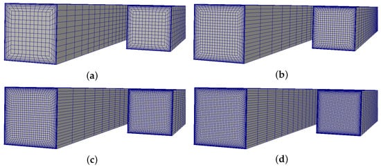
Figure 5. The inlet and outlet surfaces of the meshes: (a) coarse, (b) medium, (c) fine and (d) extra fine.

The values of the objective function and velocity profiles at three different locations are compared with all grid levels to make sure the solution is independent of mesh resolution. These velocity profiles, including both streamwise and radial directions, are taken one at the ${90}^{\circ }$ turn region (location A) and others (location B and C) at the exit of the channel, as shown in Figure 6. Figure 7 shows a comparison of the normalised streamwise velocity profiles at locations A, B and C (along the vertical lines). The positive and negative $z/D_h$ indicates the top and bottom surfaces, respectively, from the center of the U-bend. Figure 8 shows a comparison of the normalised radial velocity profiles at locations A, B and C (along the horizontal lines). To avoid overlap and maintain clarity, we presented a coarse distribution of profile points. From the comparison, it is found that both streamwise and radial velocity profiles from the fine $\left(F\right)$ and extra fine meshes are closely matched, and hence, the solution became independent of mesh resolution. Figure 9a illusrates the variation in the normalised objective function value with all the grid levels, indicating that the fine mesh results in a difference of less than $0.1\%$ in the objective function value compared to the extra fine $\left(XF\right)$ mesh. This difference is found to be acceptable for the present study [34]; hence, the fine mesh $\left(F\right)$ is used for optimisation purposes. The steady-state nonlinear primal flow solver fully converges and the discrete adjoint solver uses the same time-marching scheme, which also fully converges with the adjoint solution. The convergence history of both flow and adjoint solution using the fine mesh is shown in Figure 9b.

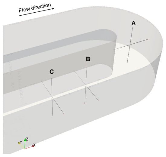
Figure 6. Locations used for velocity profiles.

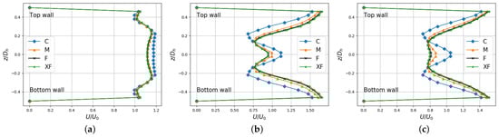
Figure 7. Streamwise velocity profiles along the vertical lines (along z axis) at (a) A, (b) B and (c) C.

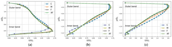
Figure 8. Radial velocity profiles along the horizontal lines (along y axis) at (a) A, (b) B and (c) C.

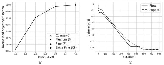
Figure 9. (a) Grid convergence study and (b) convergence history of flow and adjoint solver using fine (F) mesh.

5.4. CFD Solver Validation

The numerical results obtained using mgopt are compared with the computational and experimental ones obtained by Coletti et al. [6,9] for the same Reynolds number $Re$ = 43,830. In their experimental work, an inlet leg with length $23.3D_h$ is used to guarantee a fully developed flow at the location of the circular bend. Based on the suggestion given in the test case description [31], the inlet leg of $10D_h$ with respect to the center of the U-bend region is used in the present numerical study to reduce the computational cost.

For the validation of our present model, the simulation is performed using the fine mesh $\left(F\right)$ containing a total of 260k nodes, as the grid independence study showed that this grid offered sufficient resolution (see Figure 9b). The computed normalised axial velocity profile at the inlet section before the bend region shows very good agreement with experimental results, as illustrated in Figure 10. Figure 11 presents a comparison of the velocity field at the symmetric mid-plane simulated using the mgopt solver with experimental results by Coletti et al. [6], Large Eddy Simulation results by Alessi et al. [9] and RANS results by Alessi et al. [9]. Similar to the LES results, the mgopt solution captures the flow separation right after the turn. However, the height and length of the inner wall separation region are slightly underestimated. This underestimation is typical for RANS models, more pronounced in the results of Alessi et al. [9] compared to our results, causing lower acceleration toward the outer wall compared to the current RANS-based results.

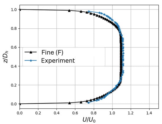
Figure 10. Comparison of normalised streamwise velocity profile taken at the inlet leg between experiment and mgopt.

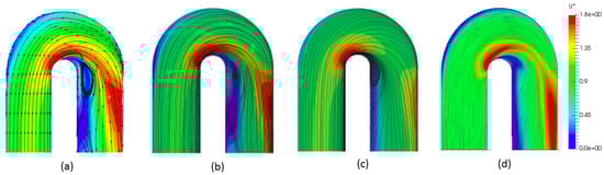
Figure 11. Comparison of normalised velocity field $\left(U^{*}\right)$ along streamwise direction between experiment and simulation taken at mid-plane. (a) Experiment [6], (b) LES simulation [9], (c) RANS simulation [9], (d) RANS-mgopt (current work).

Figure 12 shows a good agreement between mgopt and LES for the counter-rotating Dean vortices at the ${90}^{\circ }$ turn region, with only minor discrepancies observed near the inner wall separation region. This indicates that mgopt effectively captures the complex vortex structures within the turn. Furthermore, the comparison of normalised velocity magnitude at the outlet leg in Figure 13 demonstrates that mgopt results are consistent with LES results, capturing the overall flow pattern, including the interactions between the Dean vortices and the recirculation region. Thus, the fine mesh $\left(F\right)$ has been selected for the optimisation studies.

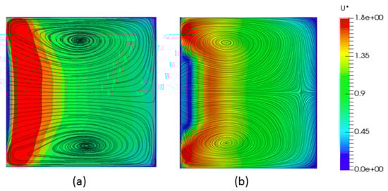
Figure 12. Comparison of normalised velocity field at ${90}^{\circ }$ turn region. (a) LES [9], (b) mgopt.

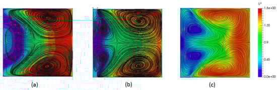
Figure 13. Comparison of normalised velocity field at outlet leg. (a) LES [9], (b) RANS [9], (c) mgopt.

5.5. Gradient Verification of Differentiated NSPCC

Since a major focus of this work is on CAD-based parametrisation, the verification of the gradient computation by Algorithmic Differentiation is presented only for the NSPCC CAD kernel; solver validation can be found in [29]. Sensitivity verification is performed by perturbing the BRep of the baseline U-bend geometry shown in Figure 1.

Ad Code vs. Complex Step Derivative

All the required derivatives of geometric operators, including surface sensitivities with respect to parameters s and t for point inversion (Equation (1)), entries of the constraint matrix $\mathbf{C}$ and CAD sensitivities (Equation (10)), are computed using derivative code produced by the source transformation AD tool Tapenade [25]. To verify the AD derivatives, we compare to the values obtained with the complex step method [35]. The method is very easy to use in Fortran, which allows very simple conversion from all double precision variables to double precision complex variables. However, additional care has been taken, as discussed in [36,37], when handling intrinsic functions such as abs and conditional branches IF..THEN..ELSE. Figure 14 shows the comparison of the convergence with step-size of the relative error in the surface sensitivity estimates using the complex step, forward, and central difference methods. The relative error here indicates the difference between the computed derivative using finite difference methods and the derivative computed using algorithmic differentiation as the reference. The rate of convergence shows that the forward difference estimate initially converges to the AD result at a linear rate, since its truncation error is $\mathcal{O}\left(h\right)$, while the central difference method converges quadratically. However, as step sizes fall below approximately ${10}^{-8}$ for forward difference and ${10}^{-7}$ for central difference, subtractive cancellation errors cause a significant increase in relative error. The complex step method is also second-order-accurate, but has no subtractive cancellation error and becomes essentially exact to machine accuracy for step sizes $\le {10}^{-8}$. This also confirms the correctness of the AD derivatives used as reference. The convergence behaviour of relative error for the complex step derivative method for seven surface points is also presented in Figure 15.

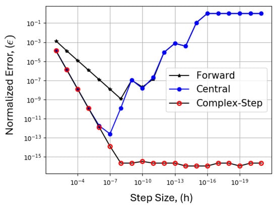
Figure 14. Convergence of relative error in the surface sensitivity estimates by complex step, forward and central difference using algorithmic differentiation result as the reference. Error: $ϵ={\displaystyle \frac{\mid FD-AD\mid }{\mid AD\mid }}$.

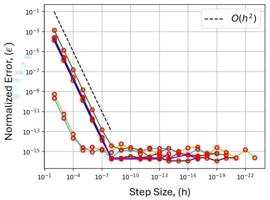
Figure 15. Convergence of relative error in the surface sensitivity for seven surface mesh points using complex step derivative (CSD) method. Each curve corresponds to a distinct mesh point on the surface. Error: $ϵ={\displaystyle \frac{\mid CSD-AD\mid }{\mid AD\mid }}$.

Additionally, the comparison of the sensitivity of the objective function with respect to control points, using shape sensitivities computed with both forward and reverse mode differentiation of the NSPCC CAD kernel, is presented in Figure 16. For visual clarity, the results are shown here for a limited number of sensitivity indices, confirming a very high degree of consistency.

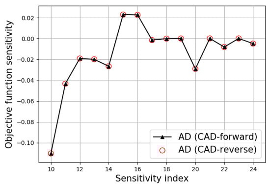
Figure 16. Comparison of sensitivity of the objective function with respect to control points $\left({\displaystyle \frac{\mathsf{\partial }J}{\mathsf{\partial }\mathbf{P}}}\right)$ with shape sensitivities computed using reverse mode and forward mode differentiation of NSPCC CAD kernel.

6. Effect of Choice of Design Space

6.1. Shape Parametrisation Using NURBS

Figure 1 shows the BRep of the U-bend geometry with design patches highlighted in green. The Boundary Representation (BRep) of the geometry consists of twelve NURBS patches: four planar rectangular patches that form the inlet and outlet channel and four curved patches that form the U-bend. $G_2$ continuity (zero curvature) is enforced at the upstream and downstream ends of the deformable part by fixing the first three layers of control points nearest to the fixed sections of the channel. $G_1$ continuity is imposed at all ‘cross-sectional’ patch interfaces, i.e., those that run mostly perpendicular to the flow between the originally planar and curved patches. $G_0$ continuity is imposed on the remaining patch interfaces that align with the flow, i.e., interfaces between originally planar patches, and originally curved patches. NSPCC derives an optimal basis for the design space from the BRep, i.e., the distribution of control points, and the choice of constraints. The number of test points to enforce the constraints is also proportional to the number of control points along that edge [24]. To show the influence of BRep control net density on aerodynamic shape optimisation, control nets for coarse (L1), medium (L2) and fine (L3) design spaces have been produced by refining globally by a factor of 2 for each level.

For the coarsest level L1, the BRep has a $6\times 4$ control net for each patch, resulting in a total of 288 control points. For L2 and L3, the BRep has an $8\times 6$ and $12\times 8$ control net for each patch, a total of 576 and 1152 control points, respectively. Control point distributions defining the U-bend region corresponding to each level are shown in Figure 17. Figure 18 shows the comparison of the shape sensitivity of a control point for each of the three levels. The BSpline representation uses a cubic spline; hence, the influence of each control point extends to the two neighbouring points in the BSpline control net either side. As the control net is refined, the support radius is reduced, enabling the representation of localised variations. The SVD then constructs an optimal and orthogonal basis of shape modes from these BSpline modes.

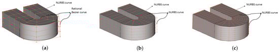
Figure 17. Levels of parametrisation: (a) coarse: level-1, (b) medium: level-2, (c) fine: level-3.

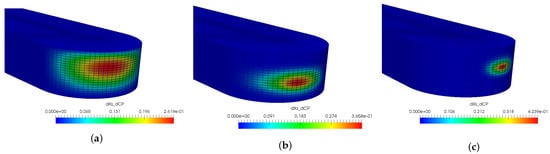
Figure 18. Shape sensitivity of a control point on the outer U-bend patch $\left({\displaystyle \frac{\mathsf{\partial }{X}_S}{\mathsf{\partial }\mathbf{P}}}\right)$: (a) coarse: level-1, (b) medium: level-2, (c) fine: level-3.

6.2. Physical Mechanisms of Total Pressure Loss Reduction

The total pressure loss in a serpentine cooling channel is primarily caused by flow separation and secondary flow generated by the turn. Figure 19 and Figure 20a show the flow field of the baseline geometry using the surface line integral convolution (LIC) visualisation technique [38], taken at various different locations along the channel and at the middle plane, respectively. When coolant flow passes through the U-bend, the presence of a pressure gradient toward the outer radius provides the centripetal force required to turn the flow. This results in very low static pressure close to the inner bend region. Consequently, as the flow exits the bend region, it experiences a strong adverse pressure gradient. The fluid particles very close to the inner wall have low velocity and do not have sufficient inertia to overcome the adverse pressure gradient. Hence, the flow separates from the inner wall boundary, which reduces the effective cross-section and thus increases wall friction, but also incurs additional secondary flow losses.

Figure 19. Normalised velocity field $\left(U^{*}\right)$ of the baseline geometry at $Re=4.3\times {10}^4$. CS view taken at various locations ordered from upstream to downstream.

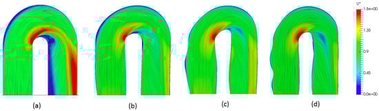
Figure 20. Comparison of normalised velocity field $\left(U^{*}\right)$ along streamwise direction between baseline and optimised geometries at $Re=4.3\times {10}^4$ taken at mid-plane. (a) Baseline, (b) opt-L1, (c) opt-L2, (d) opt-L3.

In addition to that, losses also take place due to the presence of strong secondary flows in the radial plane of the U-bend geometry because the non-uniform turbulent velocity profile is subjected to a pressure gradient normal to the streamline, which results in a non-uniform centripetal force. As a result of inertial effects, fluid at the centre of the bend moves towards the outer wall at the mid-plane and comes back towards the inner wall near the top and bottom walls (considering the bend being aligned with the horizontal). This creates symmetric strong counter-rotating vortices at the ${90}^{\circ }$ turn region, ‘Dean’ vortices, which persist in the long downstream exit channel of the U-bend, as shown in Figure 19. This strong helical motion in conjunction with the flow separation reduces the effective cross-sectional area and accelerates the flow towards the outer wall of the exit channel, which increases the velocity gradients at the wall. This in turn results in greater frictional losses in a U-bend cooling channel than the straight pipe under similar conditions, as can be clearly seen in Figure 19 and Figure 20a. A similar pattern was found in both experimental [6] and other numerical simulations [7,39]. Therefore, an effective design should be able to reduce the effects of secondary flows and flow separation in the U-bend geometry.

6.3. Shape Optimisation

Aerodynamic shape optimisation is performed using three fixed levels of parametrisation L1–L3 L1–L3. In this work, a Python-based shape optimisation framework has been developed to integrate all the required CFD and geometry modules with the Python-SciPy library to drive the design process. The overall workflow is shown in Figure 21 using an extended design structure matrix (XDSM) diagram [40]. Black lines illustrate the process flow in the order of the numbers, while gray lines represent data dependencies. At the top level, the Python API reads user-input CAD and CFD mesh files, defines the objective function, design patches, and constraint functions, and interfaces with multiple external modules for optimisation. These modules are mgopt for flow fields and CFD sensitivity computation; NSPCC for surface mesh mapping, shape perturbation, surface mesh deformation, shape sensitivity and constraint Jacobian computation; IDW for volume mesh deformation, which takes surface mesh displacements from NSPCC and smoothly propagates to the volume mesh using the inverse distance weighting method. Scipy optimise is used for optimiser selection.

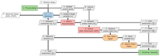
Figure 21. Shape optimisation workflow using extended design structure matrix (XDSM).

Figure 22 shows a comparison of the convergence histories of the objective function for all three levels of optimisation. The optimisation is conducted with Steepest Descent (SD). While SD typically shows very poor convergence rate for larger systems, the rate is very acceptable with NSPCC due to the orthogonality of the shape modes. To demonstrate the difference, the finest level L3 was restarted using BFGS after 64 iterations, as shown by the arrow in Figure 22. BFGS reconstructs Hessian information by matching function value and gradient evaluations at past iterates. This in turn requires that the number and definition of the design variables remain the same at each iteration. We hence keep the linearisation of $\mathrm{Ker}\left(\mathbf{C}\right)$ and its SVD constant for a number of iterates, then re-evaluate $\mathrm{Ker}\left(\mathbf{C}\right)$ and its SVD and restart BFGS. It can be observed that the convergence rate of the BFGS section from iteration 65 on L3 is not noticeably improved over the rate of SD up to iteration 64.

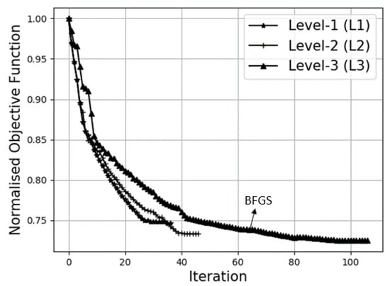
Figure 22. Comparison of objective function convergence using Steepest Descent between three different parametrisation levels. L1, L2 and L3 have 288, 576 and 1152 BSpline control points. L3 was restarted after 64 design iterations using BFGS.

Table 2 shows the percentage drop of the converged optimal designs as a function of a total number of free control points and total number of design variables offered by the NSPCC approach. For all the levels, we select a cut-off for the singular value at ${10}^{-10}$. As the design space dimension increases, the pressure loss of the optimal geometries improves, with L3 performing best. More details about the SVD cut-off and its influence on the shape optimisation can be found in [24].

Table 2. Aerodynamic shape optimisation results.

Level	Dimension	Reynolds Number	Total No. of Free Control Points (N)	Size of the Design Space	Percentage Drop in Total Pressure Loss
L1	3-D	$4.3\times {10}^4$	192	442	−25.34%
L2	3-D	$4.3\times {10}^4$	432	1082	−26.67%
L3	3-D	$4.3\times {10}^4$	576	2100	−27.52%

6.4. Flowfield of the Optimised Geometry

When compared with the baseline configuration, the optimised geometries obtained with all levels of parametrisation suppress the flow separation near the inner wall of the exit channel and reduce the wall shear stress significantly. Figure 20 shows the comparison of velocity magnitude at the mid symmetry plane between baseline and optimised geometries. The reason for the design improvement is threefold. Firstly, all levels of parametrisation increase the radius of the inner U-bend, as shown in Figure 23. For incompressible and irrotational flow, the velocity gradient normal to the streamline is proportional to the curvature of the streamline. Hence, the optimised geometries with an enlarged radius of curvature reduce the required radial pressure gradient and consequently the streamwise adverse pressure gradient, resulting in a smaller separation zone. Secondly, the duct section is considerably enlarged for all of the optimised geometries; this can be clearly seen in Figure 24, which compares the U-bend region between baseline and optimum geometries. This enlargement reduces the velocity in the bend, which, like the radius increase, reduces the required centripetal forces, and hence the required radial pressure gradient and the separation zone.

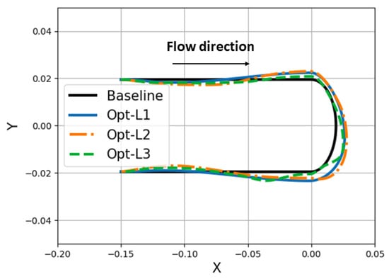
Figure 23. Comparison of inner bend radius between baseline and optimised geometries.

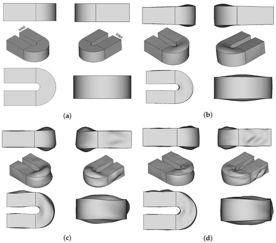
Figure 24. Comparison of design patches of the optimised U-bend region obtained using three levels of parametrisation. (a) Baseline, (b) Opt-L1, (c) Opt-L2, (d) Opt-L3.

Finally, a third contribution is the presence of surface undulations along the outer wall of the inlet channel that span from the inlet of the design surface to right before the sharp ${90}^{\circ }$ turn region. While the baseline flow and geometry are symmetric in the vertical (considering the U-bend arranged in the horizontal), a clear downward direction is observed in L3, resulting in the asymmetry of the Dean vortices, as seen at the ${90}^{\circ }$ cross-section in Figure 25, which shows the comparison of the secondary flows taken at different locations along the inlet and exit channel. It is apparent that the function of the surface undulations is similar to guide vanes used in curved flow channels and also resembles paired ridges in the venom channel of a spitting cobra, which reduces pressure loss [41]. The downward direction of the bumps pre-conditions the flow with a dominant counter-clockwise swirl (when viewed in the flow direction). Only the L3 parametrisation includes shape modes that are local enough to express the wall undulations needed to achieve this.

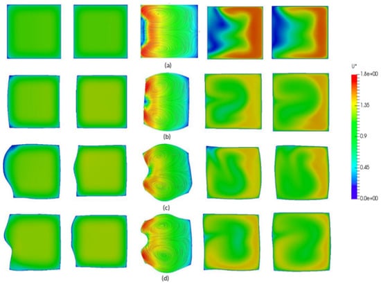
Figure 25. Comparison of normalised velocity field $\left(U^{*}\right)$ between optimised geometries at $Re=4.3\times {10}^4$. Cross-sectional (CS) views taken at various locations ordered from upstream to downstream. (a) Baseline, (b) Opt-L1, (c) Opt-L2, (d) Opt-L3.

The flow in the baseline geometry shows a very non-uniform velocity distribution in the 90${}^{\circ }$ section, with a large region of low velocity near the inner bend, resulting in an effectively reduced cross-section and higher viscous losses. The optimised shapes suppress the low-velocity region. The span of the shape modes of L1 is wide enough to span the entire channel height, and the inner radius of L1 is changed uniformly. The locality of the shape modes in L2 and L3 enables it to pick up a shape feature that varies the radius and height, effectively shaping the upper and lower halves of the bend cross-sections to ‘mold’ around the secondary flow features. This increases the frictional resistance to the secondary flow, while also using the momentum of the secondary flow to energise and/or displace the low-velocity region near the inner radius. The most significant gains in pressure loss of 25.34% are achieved already with the coarsest L1 parametrisation. Further refinements to L2 and L3 gain another 1.3% from L1 to L2, and another 0.9% from L2 to L3; see Table 2. Further refinement of the control net might reduce the pressure slightly further, but could also reduce the locality of the shape mode to a scale comparable with the computational grid, which in turn might require additional surface regularisation techniques to filter out unwanted high-frequency modes that are not penalised by the flow model. Many existing studies on the VKI U-bend test case often simplify constraint formulations and use inconsistent Reynolds number, which makes direct comparisons with our results misleading. Each work uses its own flow solver and uses different RANS turbulence models. Most importantly, we use a total pressure and total temperature inlet condition typical for compressible turbomachinery flow, while the other works use a velocity inlet condition that fixes mass flow. In our optimisation, mass flow increases as the total pressure loss is reduced. Therefore, we chose not to include comparisons with other available results over total pressure loss reduction in Table 2.

6.5. Off-Design Performance

The highly refined shape of L3 may be optimal only for a particular Reynolds number, while the design may seek good performance across a range of flow speeds. To study the effect of Reynolds number, the performance of the designs is evaluated using a range of Reynolds numbers from $1\times {10}^4$ to $7\times {10}^4$. The effect of Reynolds number on the value of the objective function is shown in Figure 26, with the value of the objective function normalised by the value for the baseline case. All optimal geometries retain their improved performance over the entire range of Reynolds numbers, although the improvement for the L3 shape is diminished when compared to the L1 and L2 shapes at lower and higher Reynolds numbers.

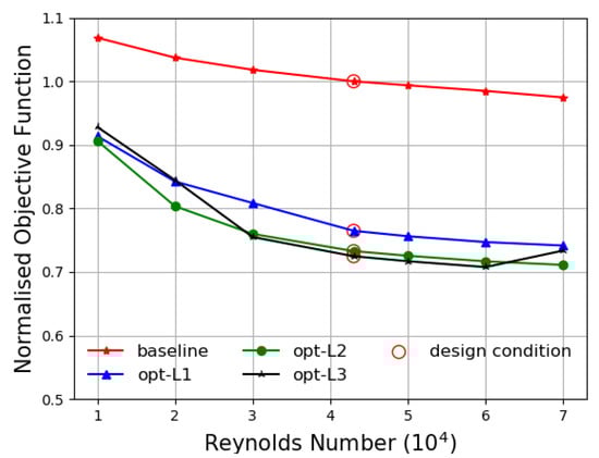
Figure 26. Influence of Reynolds number on the objective function value.

6.6. Computational Time

To analyse the computational cost of the various steps within a design iteration, the runtime of each of these steps is shown in Table 3 for three levels of parametrisation. Timings are taken for the first design step in which the primal and adjoint CFD solves up to full convergence. The optimisation process is performed using the fine (F) mesh with 260k nodes. The data show that the dominant cost arises from the primal and adjoint CFD computation, while the cost associated with the shape parametrisation and optimisation is negligibly small in comparison. In this work, shape sensitivities are obtained using reverse mode differentiation. For the case of conformal NURBS patches, both forward and reverse mode differentiation are fine. However in the case of non-conformal, when the intersection has to be computed, the surface grid must be smoothed and reprojected [42], leading to higher costs associated with shape derivatives. Hence, reverse mode differentiation might be beneficial in such cases.

Table 3. Computational time breakdown for a single design step.

Computation	Percentage over Total Time
	L1	L2	L3
Primal	44.99	44.87	44.74
Adjoint	54.75	54.59	54.43
Surface Mesh Mapping	0.16	0.22	0.33
SVD null space	0.05	0.22	0.34
CAD perturbation	0.01	0.01	0.02
Constraint recovery	0.02	0.05	0.11

7. Conclusions and Future Work

The NSPCC approach derives smooth orthogonal shape modes directly from the boundary representation of a CAD model and chosen constraints. This study extended and differentiated the NSPCC method in adjoint mode to efficiently handle high-fidelity design spaces for gradient-based shape optimisation. We further investigated the impact of varying control net densities on NURBS patches with nonlinear constraints on the optimal shape of the benchmark VKI U-bend internal turbine blade cooling channel. The optimisation was conducted using three different levels of parametrisation: L1, L2, and L3, with 192, 432, and 576 free control points, respectively, resulting in design spaces of 442, 1082, and 2100 degrees of freedom (DoF) for the three levels.

The density of control points on the NURBS patches significantly influences the shape modes captured during the design process, affecting both the optimal solution and the convergence rate of the optimisation. The finer levels L2 and L3 exhibit increased modulation of the surface, effectively reducing pressure losses due to secondary flow. This is evident in the deformation of the cross-section at the mid-bend, resulting in a W-shape of the inner radius with a pronounced increase at mid-height. Most notably, downward ridges emerge on L3 on the outer radius upstream of the bend, a feature also observable at a coarser resolution on L2. Despite the initial symmetry with respect to the horizontal mid-plane, the optimisation finds improvement through non-symmetric shape variations. This feature ‘pre-conditions’ the flow with secondary motion before it enters the bend, ultimately reducing secondary flow losses. Notably, this pattern has not been observed in previous U-bend benchmark studies, highlighting NSPCC’s capability to parametrise a high-dimensional design space with orthogonal shape modes crucial for converging complex shape optimisation problems.

It has been shown that the NSPCC approach is able to generate rich design and well-conditioned design spaces, crucial for capturing all significant shape modes without constraining the design flexibility and ensuring converged shape optimisation results. This approach is suitable for any complex industrial shape optimisation applications and has many advantages:

• Local shape control with orthogonal modes: The local support of B-Splines enables us to concentrate shape modes to deform only local areas. NSPCC computes an orthogonal basis for this design space, thus ensuring convergence of the optimisation in the case of very fine control nets as well.
• Smoothness: The B-Spline surfaces are smooth by construction up to the desired level of differentiability.
• Efficient constraint handling: Geometric constraints, such geometric continuity across NURBS patch interfaces ($G_0,$ $G_1$ and $G_2$) or thickness, curvature and box constraints can be imposed using the test point approach of NSPCC and are included in the orthogonalisation of the basis for the design space.
• Exact and Efficient CAD sensitivities: The NSPCC CAD kernel is differentiated using source transformation tool TAPENADE providing exact CAD sensitivities regardless of the local scaling of the geometry. The CAD kernel has been also differentiated in reverse mode, enabling it to compute the complete sensitivity of the objective function w.r.t. the design parameters in a single calculation, irrespective of the size of the design space.
• Portability: The NSPCC approach preserves the topology of the CAD model and consistently updates the parameters of the model in the design loop. The optimal shape is then available as a CAD geometry to support meshing for further multi-disciplinary analyses, but also to serve as an exact datum surface for multi-disciplinary coupling.

In this study, the control net levels remain fixed for each optimisation process. Our future work will focus on implementing adaptive control point refinement of NURBS patches to enhance the design space resolution in areas of high sensitivity. Additionally, we plan to expand the application to accommodate multi-objective functions, addressing both fluid flow dynamics and conjugate heat transfer analysis.

References

- Yu, Y.; Lyu, Z.; Xu, Z.; Martins, J.R. On the influence of optimization algorithm and initial design on wing aerodynamic shape optimization. Aerosp. Sci. Technol. 2018, 75, 183–199. [Google Scholar] [CrossRef]
- Jameson, A. Optimum aerodynamic design using CFD and control theory. AIAA Pap. 1995, 1729, 124–131. [Google Scholar]
- Schmidt, S.; Ilic, C.; Gauger, N.; Schulz, V. Shape Gradients and Their Smoothness for Practical Aerodynamic Design Optimization; DFG SFB 1253 Preprint-Number SPP1253-10-03; Universität Erlangen: Erlangen, Germany, 2008. [Google Scholar]
- Hojjat, M.; Stavropoulou, E.; Bletzinger, K.U. The Vertex Morphing method for node-based shape optimization. Comput. Methods Appl. Mech. Eng. 2014, 268, 494–513. [Google Scholar] [CrossRef]
- Jaworski, A.; Müller, J.D. Toward modular multigrid design optimisation. In Proceedings of the Lecture Notes in Computational Science and Engineering; Bischof, C., Utke, J., Eds.; Springer: New York, NY, USA, 2008; Volume 64, pp. 281–291. [Google Scholar]
- Coletti, F.; Verstraete, T.; Bulle, J.; Van der Wielen, T.; Van den Berge, N.; Arts, T. Optimization of a U-Bend for Minimal Pressure Loss in Internal Cooling Channels-Part II: Experimental Validation. J. Turbomach. 2013, 135, 051016. [Google Scholar] [CrossRef]
- Verstraete, T.; Coletti, F.; Bulle, J.; Vanderwielen, T.; Arts, T. Optimization of a U-Bend for Minimal Pressure Loss in Internal Cooling Channels Part I: Numerical Method. J. Turbomach. 2013, 135, 051015. [Google Scholar] [CrossRef]
- Namgoong, H.; Ireland, P.; Son, C. Optimisation of a 180° U-shaped bend shape for a turbine blade cooling passage leading to a pressure loss coefficient of approximately 0.6. Proc. Inst. Mech. Eng. Part G J. Aerosp. Eng. 2016, 230, 1371–1384. [Google Scholar] [CrossRef]
- Alessi, G.; Verstraete, T.; Koloszar, L.; van Beeck, J.P.A.J. Comparison of large eddy simulation and Reynolds-averaged Navier–Stokes evaluations with experimental tests on U-bend duct geometry. Proc. Inst. Mech. Eng. Part A J. Power Energy 2020, 234, 315–322. [Google Scholar] [CrossRef]
- Kiyici, F.; Yilmazturk, S.; Arican, E.; Costa, E.; Porziani, S. U-turn optimization of a ribbed turbine blade cooling channel using a meshless optimization technique. In Proceedings of the 55th AIAA Aerospace Sciences Meeting, Grapevine, TX, USA, 9–13 January 2017; p. 1534. [Google Scholar]
- Willeke, S.; Verstraete, T. Adjoint Optimization of an Internal Cooling Channel U-Bend. In Proceedings of the ASME Turbo Expo 2015: Turbine Technical Conference and Exposition. American Society of Mechanical Engineers, Montreal, QC, Canada, 15–19 June 2015. [Google Scholar]
- He, P.; Mader, C.A.; Martins, J.R.; Maki, K.J. Aerothermal optimization of a ribbed U-bend cooling channel using the adjoint method. Int. J. Heat Mass Transf. 2019, 140, 152–172. [Google Scholar] [CrossRef]
- Verstraete, T.; Müller, L.; Müller, J.D. Adjoint-based design optimisation of an internal cooling channel U-bend for minimised pressure losses. Int. J. Turbomach. Propuls. Power 2017, 2, 10. [Google Scholar] [CrossRef]
- Kim, C.; Son, C. Rapid design approach for U-bend of a turbine serpentine cooling passage. Aerosp. Sci. Technol. 2019, 92, 417–428. [Google Scholar] [CrossRef]
- Alessi, G.; Verstraete, T.; Koloszar, L.; Blocken, B.; van Beeck, J. Adjoint shape optimization coupled with LES-adapted RANS of a U-bend duct for pressure loss reduction. Comput. Fluids 2021, 228, 105057. [Google Scholar] [CrossRef]
- Robinson, T.; Armstrong, C.; Chua, H.; Othmer, C.; Grahs, T. Optimizing Parameterized CAD Geometries Using Sensitivities Based on Adjoint Functions. Comput.-Aided Des. Appl. 2012, 9, 253–268. [Google Scholar] [CrossRef]
- Agarwal, D.; Christos, K.; Robinson, T.T.; Armstrong, C.G. Using Parametric Effectiveness for Efficient CAD-Based Adjoint Optimization. Comput. Aided Des. Appl. 2019, 16, 703–719. [Google Scholar] [CrossRef]
- Dannenhoffer, J.; Haimes, R. Design sensitivity calculations directly on CAD-based geometry. In Proceedings of the 53rd AIAA Aerospace Sciences Meeting, Kissimmee, FL, USA, 5–9 January 2015; p. 1370. [Google Scholar]
- Auriemma, S. Applications of differentiated CAD kernel in gradient-based aerodynamic shape optimisation. In Proceedings of the 2018 Joint Propulsion Conference, Cincinnati, OH, USA, 9–11 July 2018; p. 4828. [Google Scholar]
- Banović, M.; Mykhaskiv, O.; Auriemma, S.; Walther, A.; Legrand, H.; Müller, J.D. Algorithmic differentiation of the Open CASCADE Technology CAD kernel and its coupling with an adjoint CFD solver. Optim. Methods Softw. 2018, 33, 813–828. [Google Scholar] [CrossRef]
- Mueller, J.; Banovic, M.; Auriemma, S.; Mohanamuraly, P.; Walther, A.; Legrand, H. NURBS-based and Parametric-based Shape Optimisation with differentiated CAD Kernel. Comput.-Aided Des. Appl. 2018, 15, 916–926. [Google Scholar]
- He, P.; Mader, C.A.; Martins, J.; Maki, K. Aerothermal optimization of internal cooling passages using a discrete adjoint method. In Proceedings of the 2018 Joint Thermophysics and Heat Transfer Conference, Atlanta, GA, USA, 25–29 June 2018; p. 4080. [Google Scholar]
- Jesudasan, R.; Zhang, X.; Mueller, J.D. Adjoint optimisation of internal turbine cooling channel using NURBS-based automatic and adaptive parametrisation method. In Proceedings of the ASME 2017 Gas Turbine India Conference, American Society of Mechanical Engineers, Bangalore, India, 7–8 December 2017; p. V001T02A009. [Google Scholar]
- Müller, J.D.; Zhang, X.; Akbarzadeh, S.; Wang, Y. Geometric continuity constraints of automatically derived parametrisations in CAD-based shape optimisation. Int. J. Comput. Fluid Dyn. 2019, 33, 272–288. [Google Scholar] [CrossRef]
- Hascoët, L.; Pascual, V. The Tapenade Automatic Differentiation tool: Principles, Model, and Specification. ACM Trans. Math. Softw. 2013, 39, 1–43. [Google Scholar] [CrossRef]
- Xu, S.; Jahn, W.; Müller, J.D. CAD-based shape optimisation with CFD using a discrete adjoint. Int. J. Numer. Methods Fluids 2013, 74, 153–168. [Google Scholar] [CrossRef]
- Piegl, L.; Tiller, W. The NURBS Book; Springer Science & Business Media: Berlin/Heidelberg, Germany, 2012. [Google Scholar]
- Mueller, J.D.; Hueckelheim, J.; Mykhaskiv, O. STAMPS: A finite-volume solver framework for adjoint codes derived with source-transformation AD. In Proceedings of the 2018 Multidisciplinary Analysis and Optimization Conference, Atlanta, GA, USA, 25–29 June 2018; p. 2928. [Google Scholar]
- Gugala, M. Output-Based Mesh Adaptation Using Geometric Multi-Grid for Error Estimation. Ph.D. Thesis, School of Engineering and Materials Science, Queen Mary University of London, London, UK, 2018. [Google Scholar]
- Jaworski, A.; Müller, J.D.; Rokicki, J. One-shot optimisation with grid adaptation using adjoint sensitivities. In Proceedings of the ECCOMAS 2012, Vienna, Austria, 10–14 September 2012; pp. 3685–3693. [Google Scholar]
- Verstraete, T. The VKI U-Bend Optimization Test Case; Technical Report; The von Karman Institute for Fluid Dynamics: Sint-Genesius-Rode, Belgium, 2016. [Google Scholar]
- Xu, S.; Radford, D.; Meyer, M.; Müller, J.D. Stabilisation of discrete steady adjoint solvers. J. Comput. Phys. 2015, 299, 175–195. [Google Scholar] [CrossRef]
- Forsythe, N. A Partitioned Approach to Fluid-Structure Interaction for Artificial Heart Valves. Ph.D. Thesis, School of Mechanical and Aerospace Engineering, Queen’s University Belfast, Belfast, UK, 2006. [Google Scholar]
- McHale, M.; Friedman, J.; Karian, J. Standard for Verification and Validation in Computational Fluid Dynamics and Heat Transfer; The American Society of Mechanical Engineers, ASME V&V: New York, NY, USA, 2009; pp. 20–2009. [Google Scholar]
- Squire, W.; Trapp, G. Using Complex Variables to Estimate Derivatives of Real Functions. SIAM-Rev. 1998, 10, 110–112. [Google Scholar] [CrossRef]
- Cusdin, P. Automatic Sensitivity Code for Computational Fluid Dynamics. Ph.D. Thesis, School of Aeronautical Engineering, Queen’s University Belfast, Belfast, UK, 2005. [Google Scholar]
- Martins, J.R.; Sturdza, P.; Alonso, J.J. The complex-step derivative approximation. ACM Trans. Math. Softw. (TOMS) 2003, 29, 245–262. [Google Scholar] [CrossRef]
- Mao, X.; Kikukawa, M.; Fujita, N.; Imamiya, A. Line integral convolution for 3D surfaces. In Visualization in Scientific Computing’97, Proceedings of the Eurographics Workshop, Boulogne-sur-Mer, France, 28–30 April 1997; Springer: Berlin/Heidelberg, Germany, 1997; pp. 57–69. [Google Scholar]
- Luo, J.; Razinsky, E.H. Analysis of turbulent flow in 180 deg turning ducts with and without guide vanes. J. Turbomach. 2009, 131, 021011. [Google Scholar] [CrossRef]
- Lambe, A.B.; Martins, J.R. Extensions to the design structure matrix for the description of multidisciplinary design, analysis, and optimization processes. Struct. Multidiscip. Optim. 2012, 46, 273–284. [Google Scholar] [CrossRef]
- Triep, M.; Hess, D.; Chaves, H.; Brücker, C.; Balmert, A.; Westhoff, G.; Bleckmann, H. 3D flow in the venom channel of a spitting cobra: Do the ridges in the fangs act as fluid guide vanes? PLoS ONE 2013, 8, e61548. [Google Scholar] [CrossRef] [PubMed]
- Mykhaskiv, O.; Mohanamuraly, P.; Mueller, J.D.; Xu, S.; Timme, S. CAD-based shape optimisation of the NASA CRM wing-body intersection using differentiated CAD-kernel. In Proceedings of the 35th AIAA Applied Aerodynamics Conference, Denver, CO, USA, 5–9 June 2017; p. 4080. [Google Scholar]
Disclaimer/Publisher’s Note: The statements, opinions and data contained in all publications are solely those of the individual author(s) and contributor(s) and not of MDPI and/or the editor(s). MDPI and/or the editor(s) disclaim responsibility for any injury to people or property resulting from any ideas, methods, instructions or products referred to in the content. |
© 2024 by the authors. Licensee MDPI, Basel, Switzerland. This article is an open access article distributed under the terms and conditions of the Creative Commons Attribution (CC BY) license (https://creativecommons.org/licenses/by/4.0/).