Appendix B. Full Monthly Disaggregation Results by Region
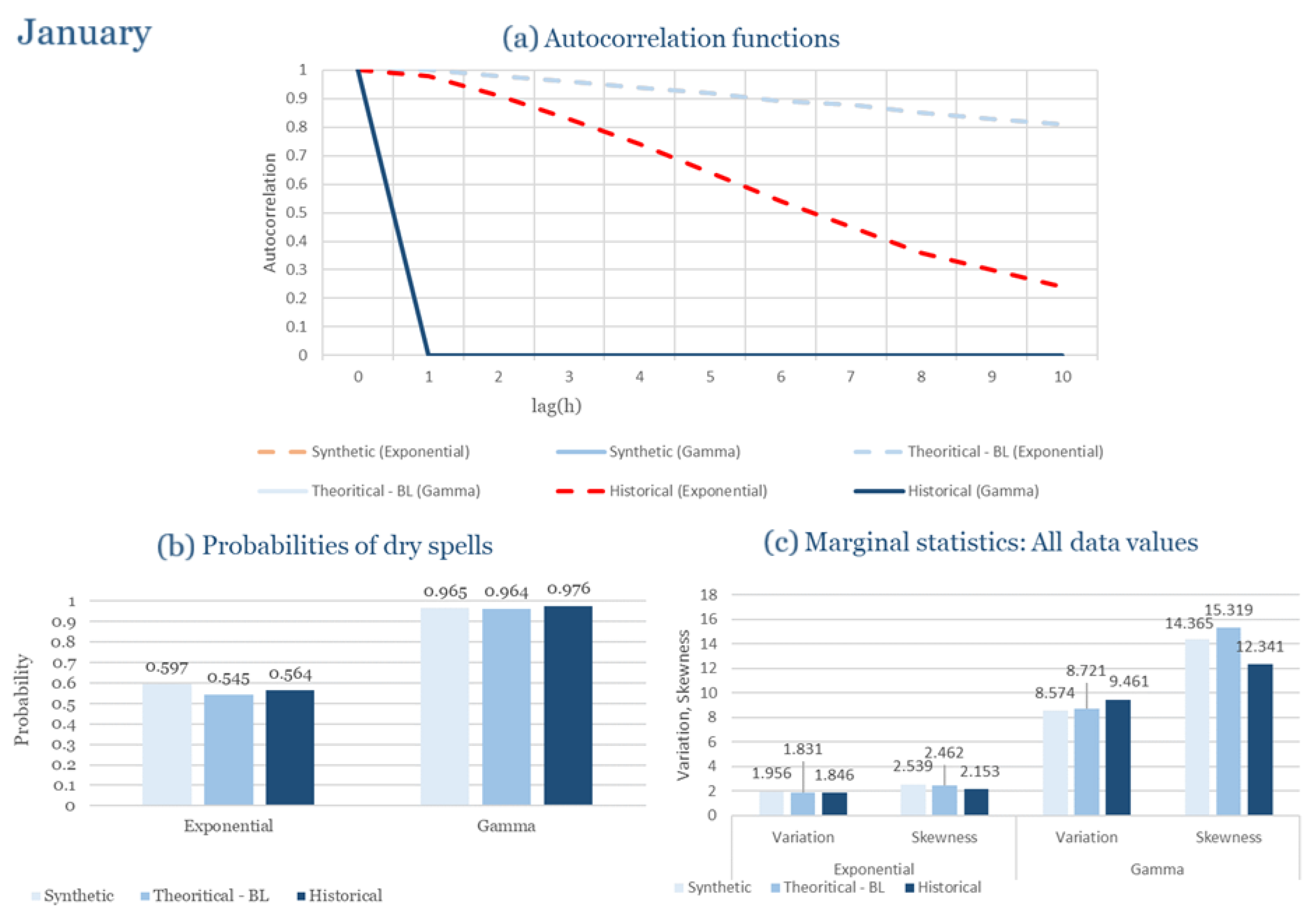
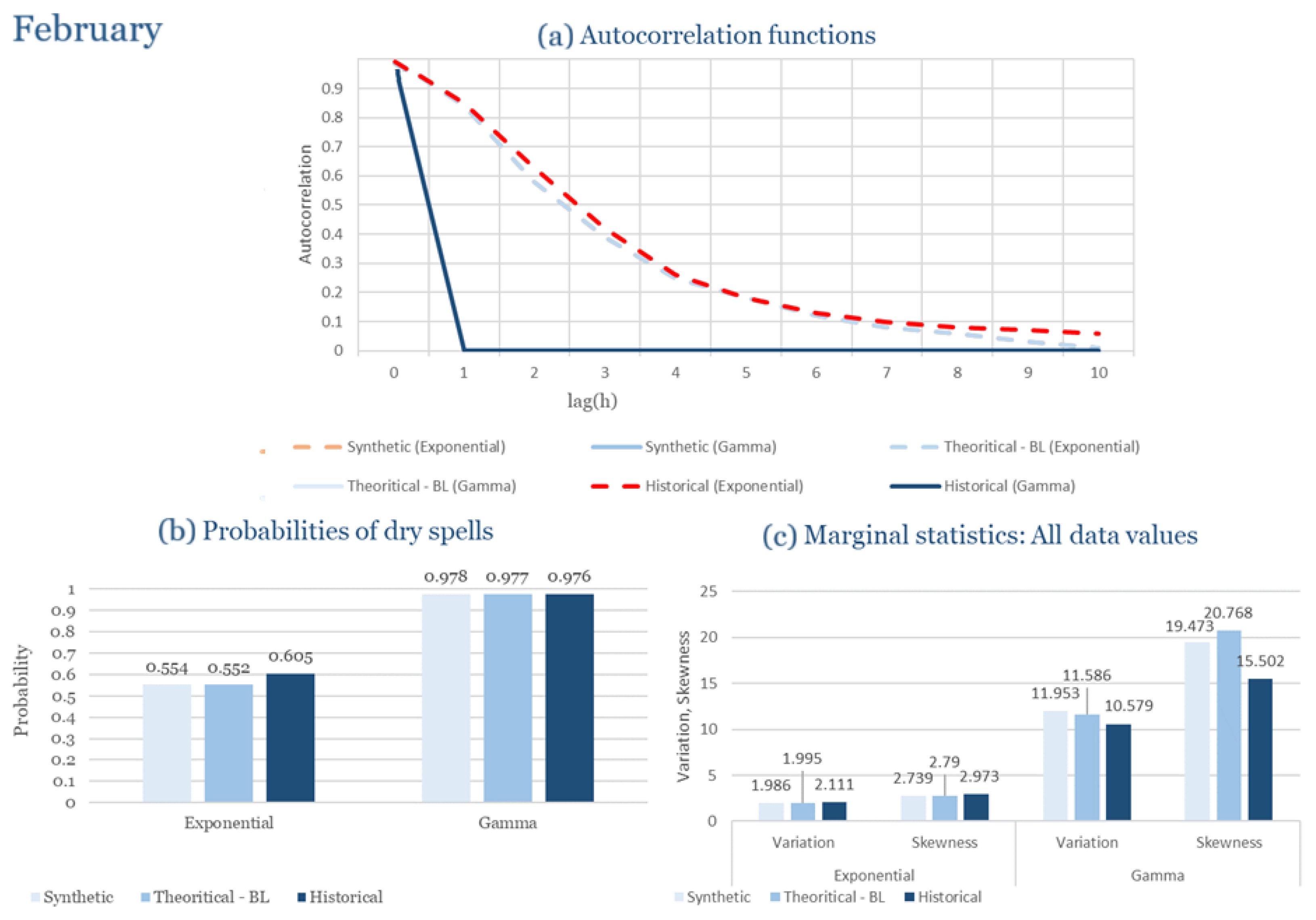
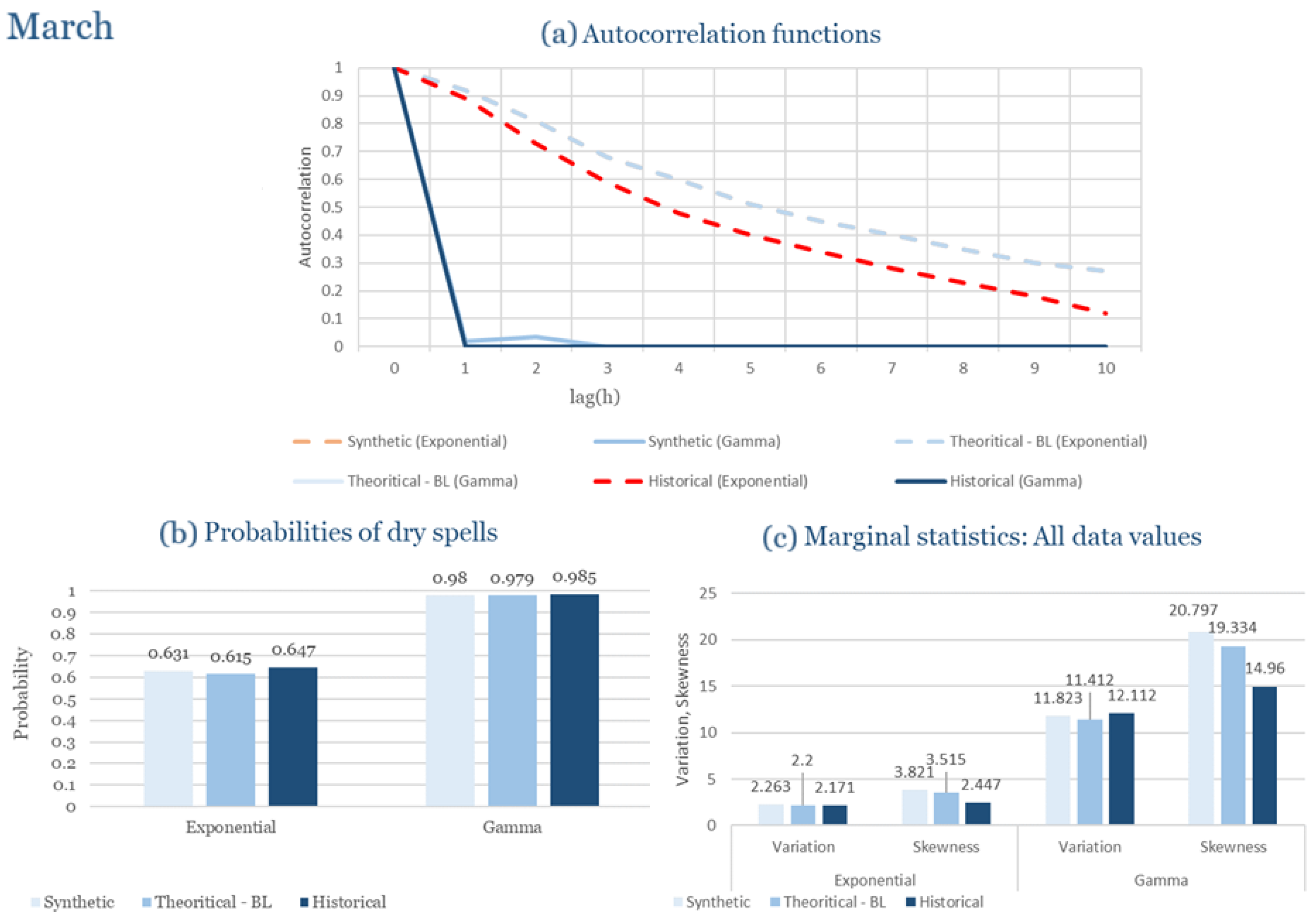
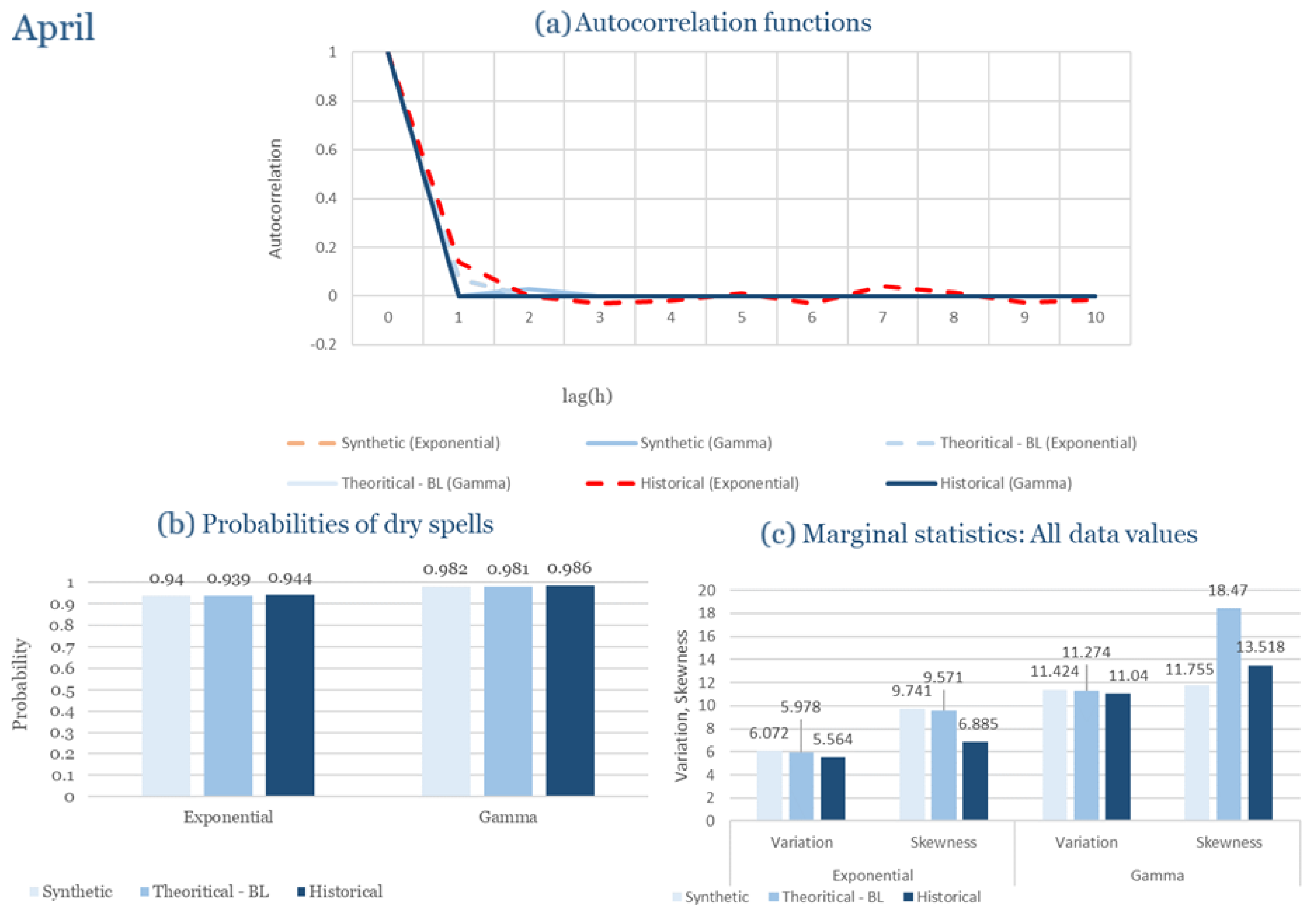
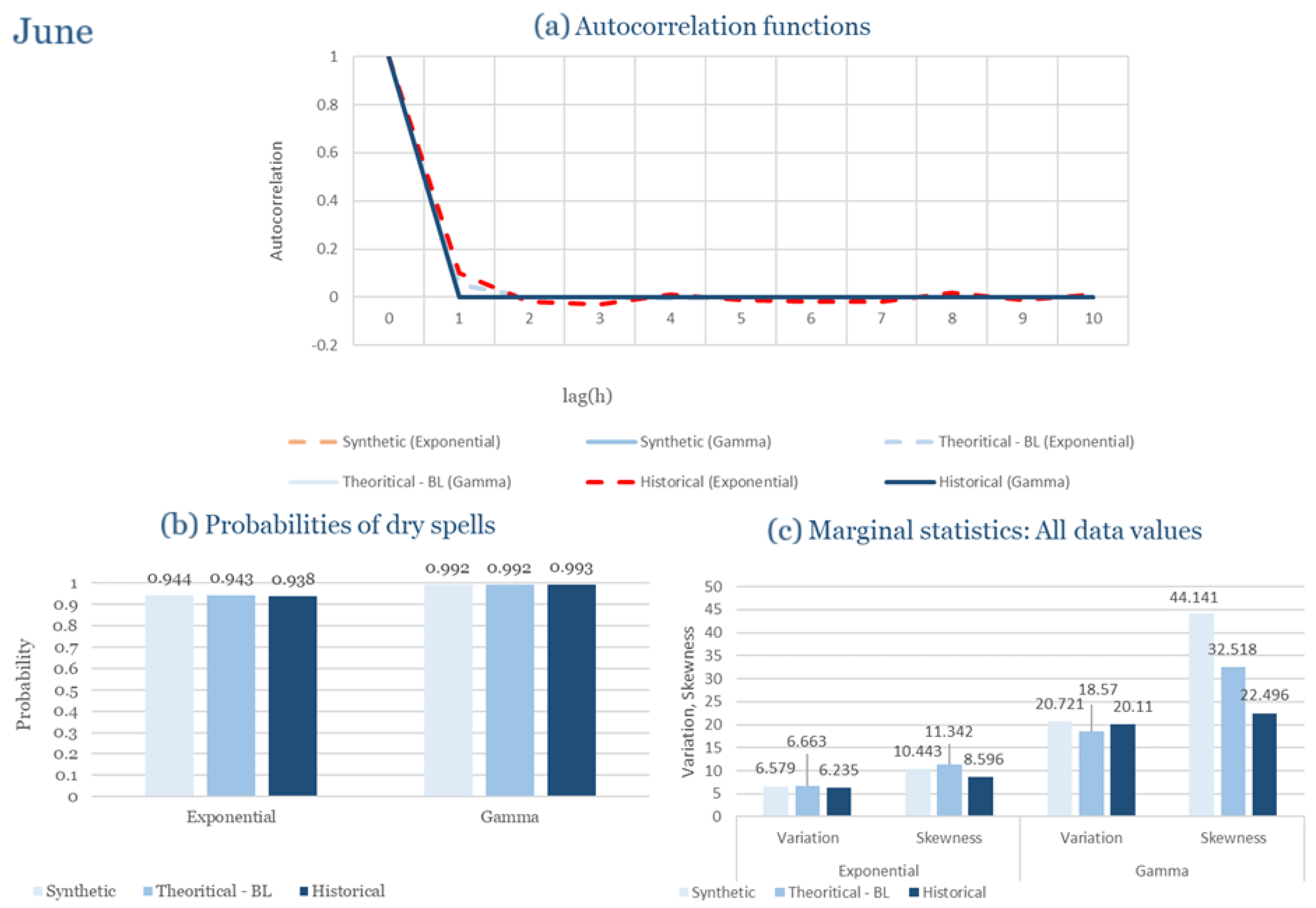
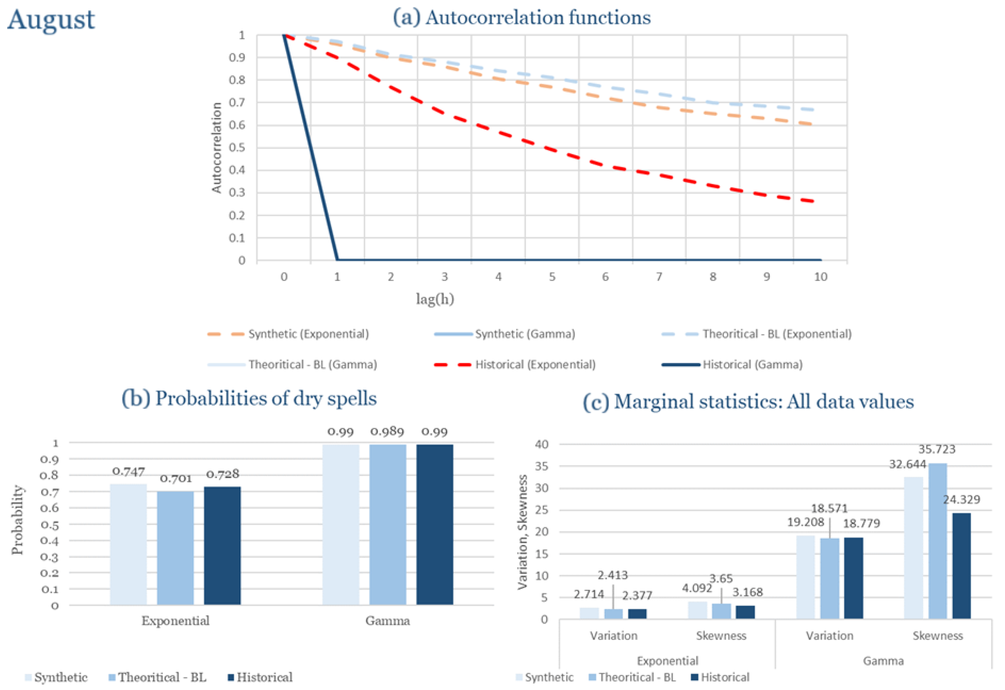
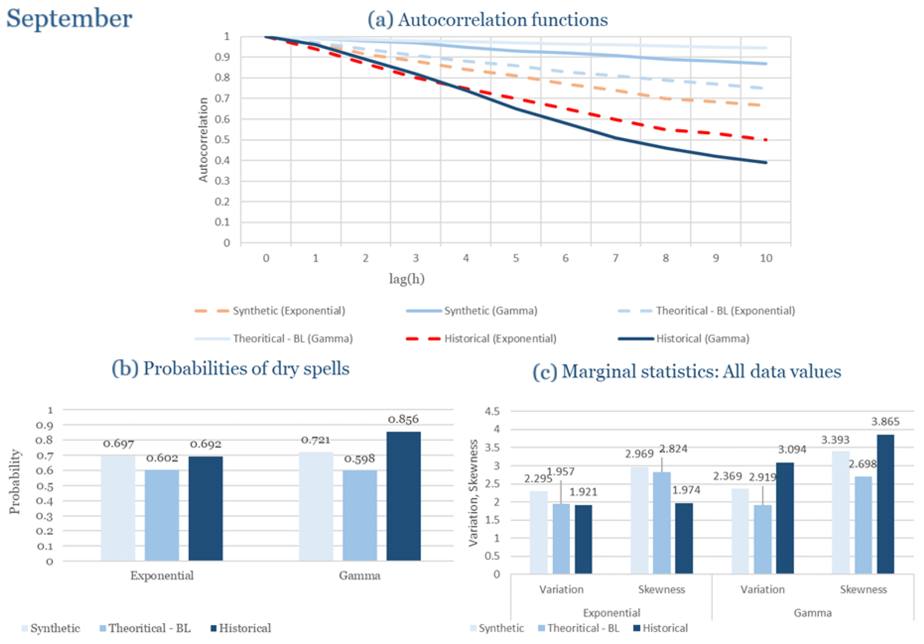
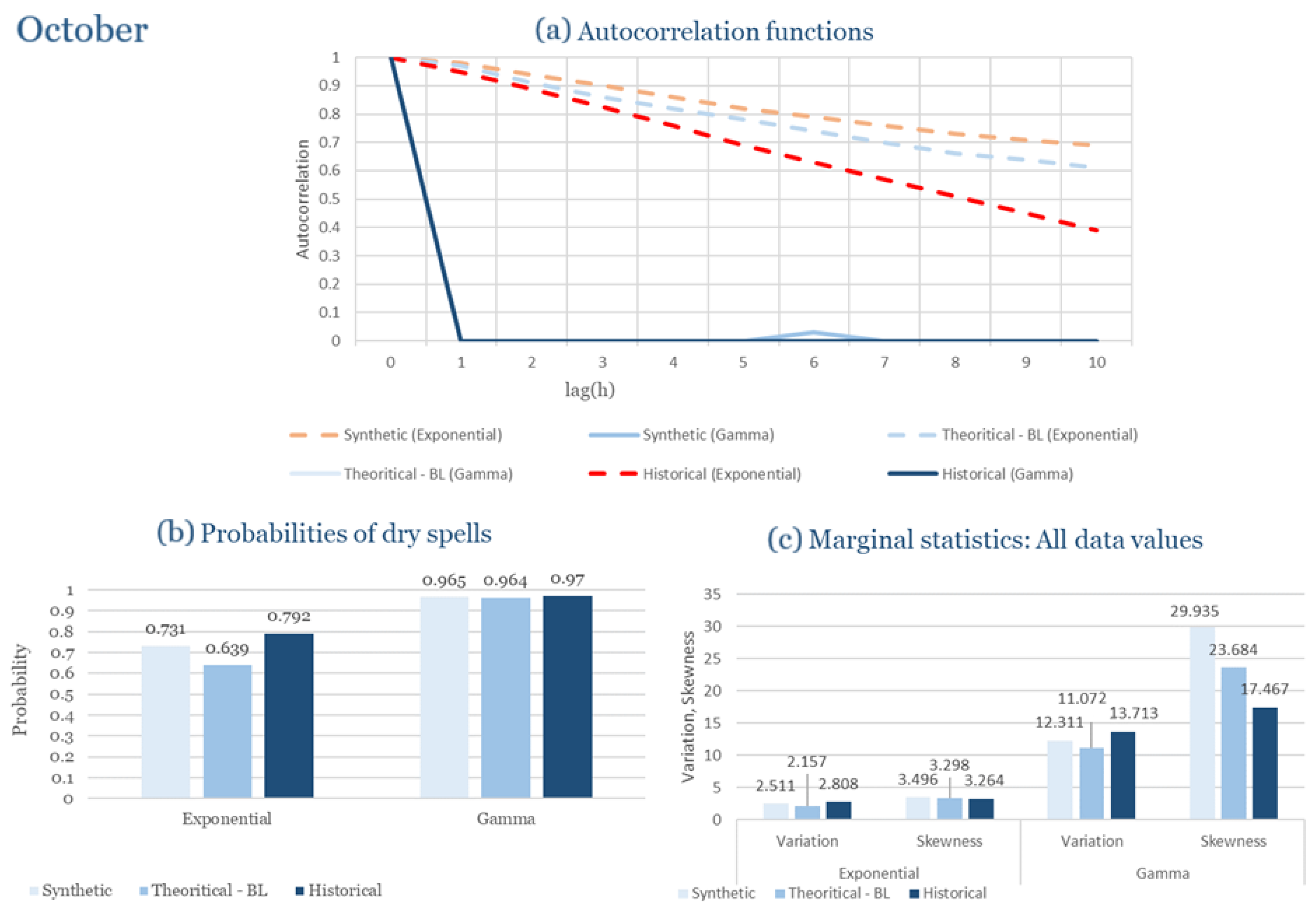
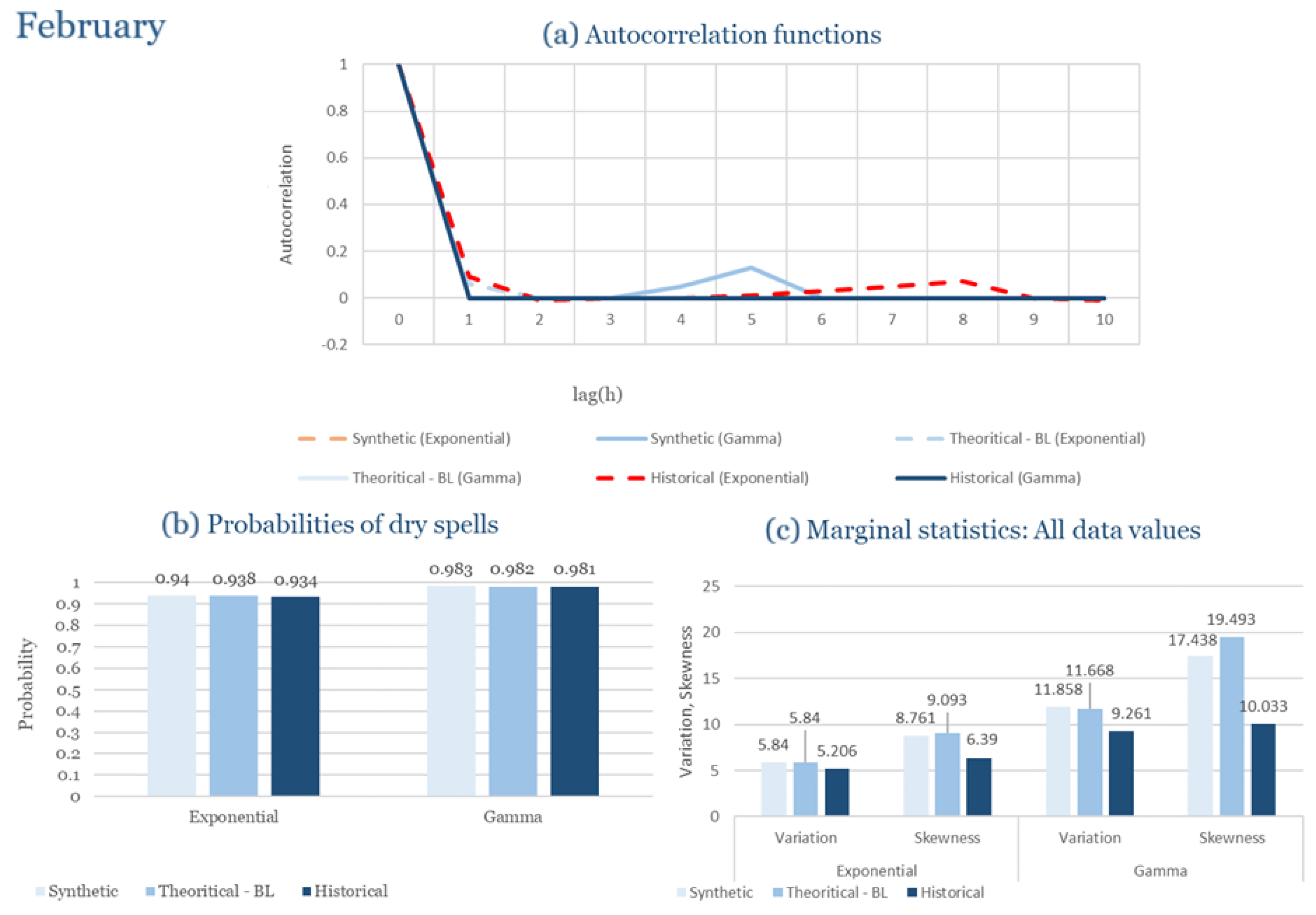
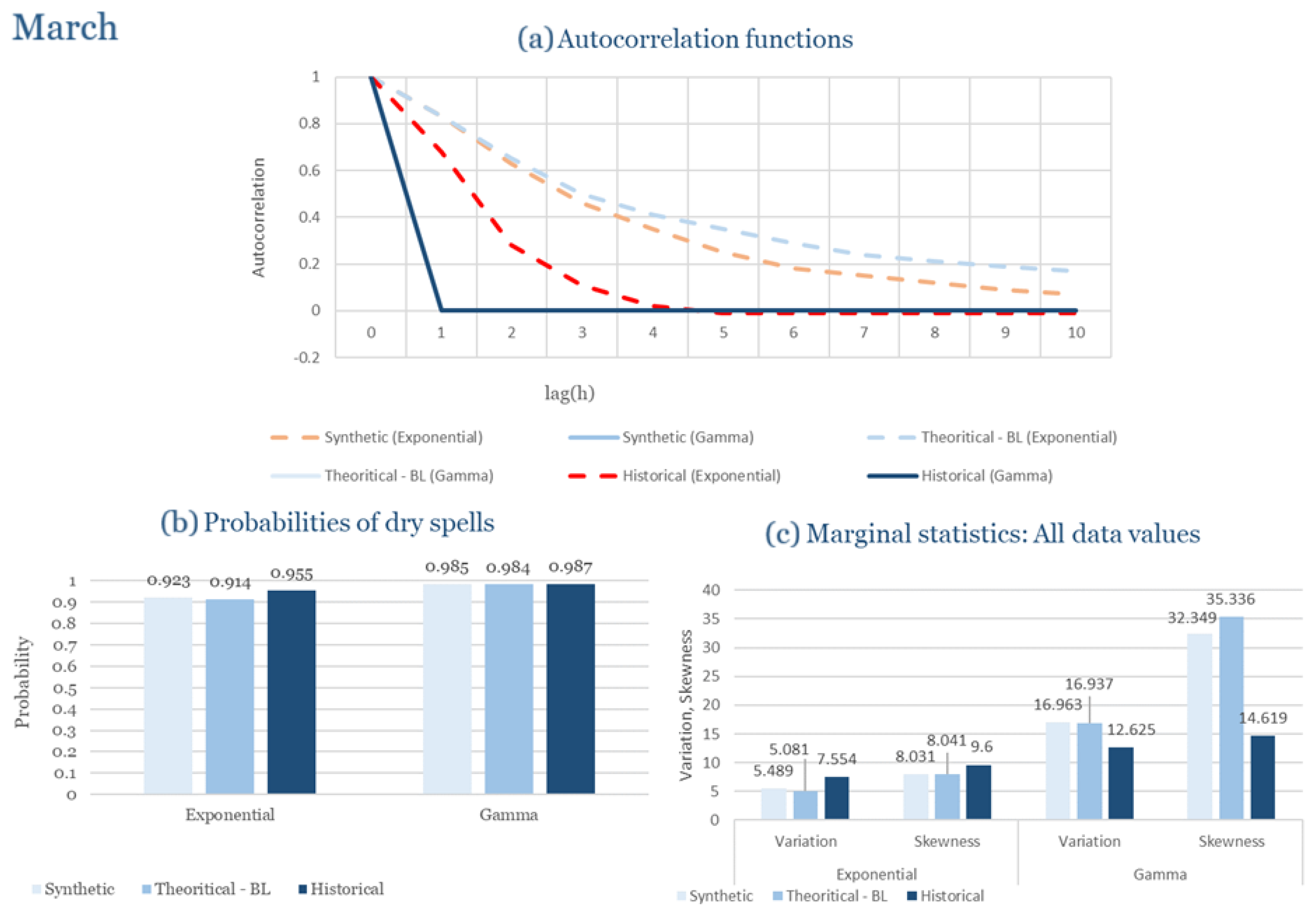
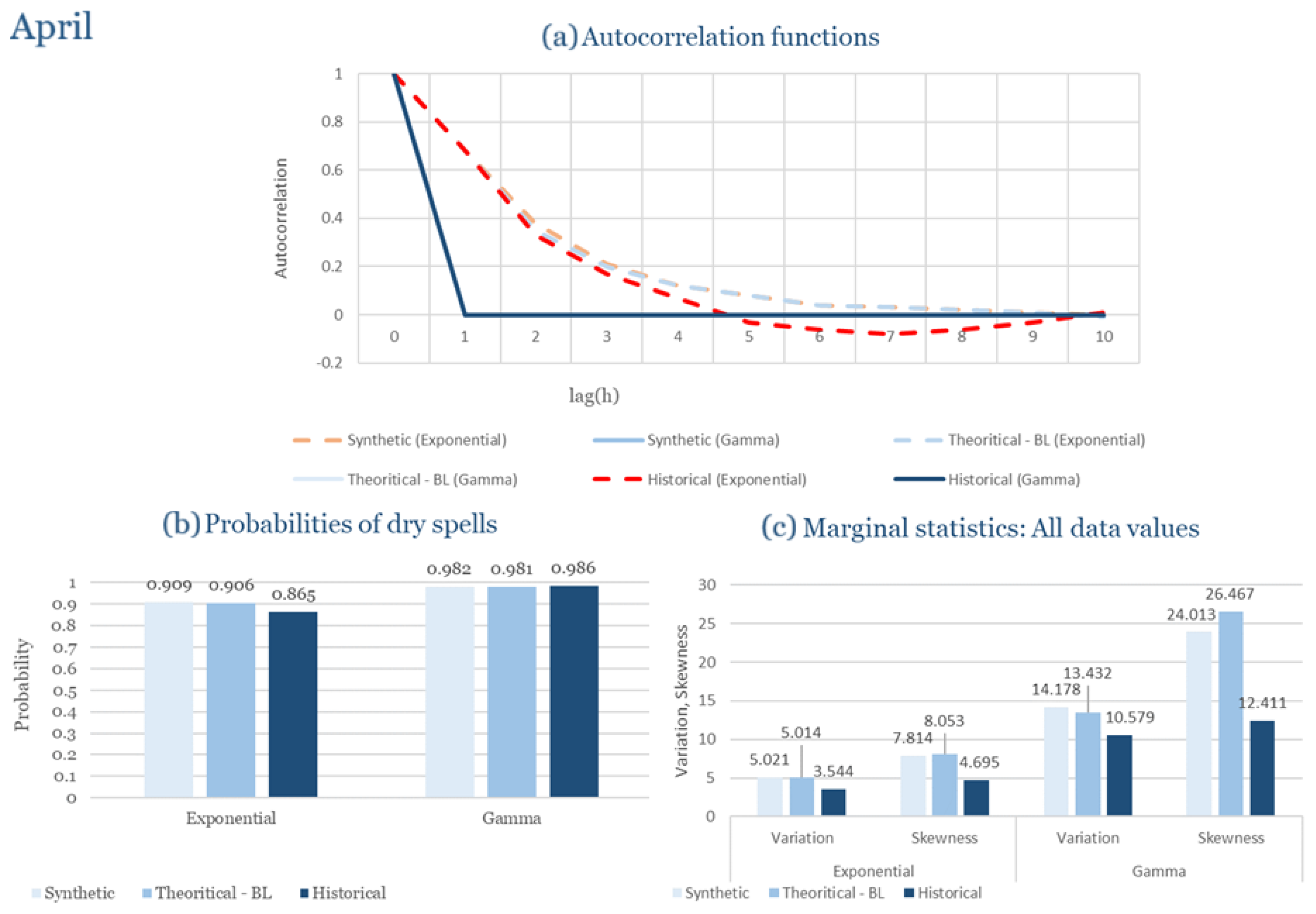
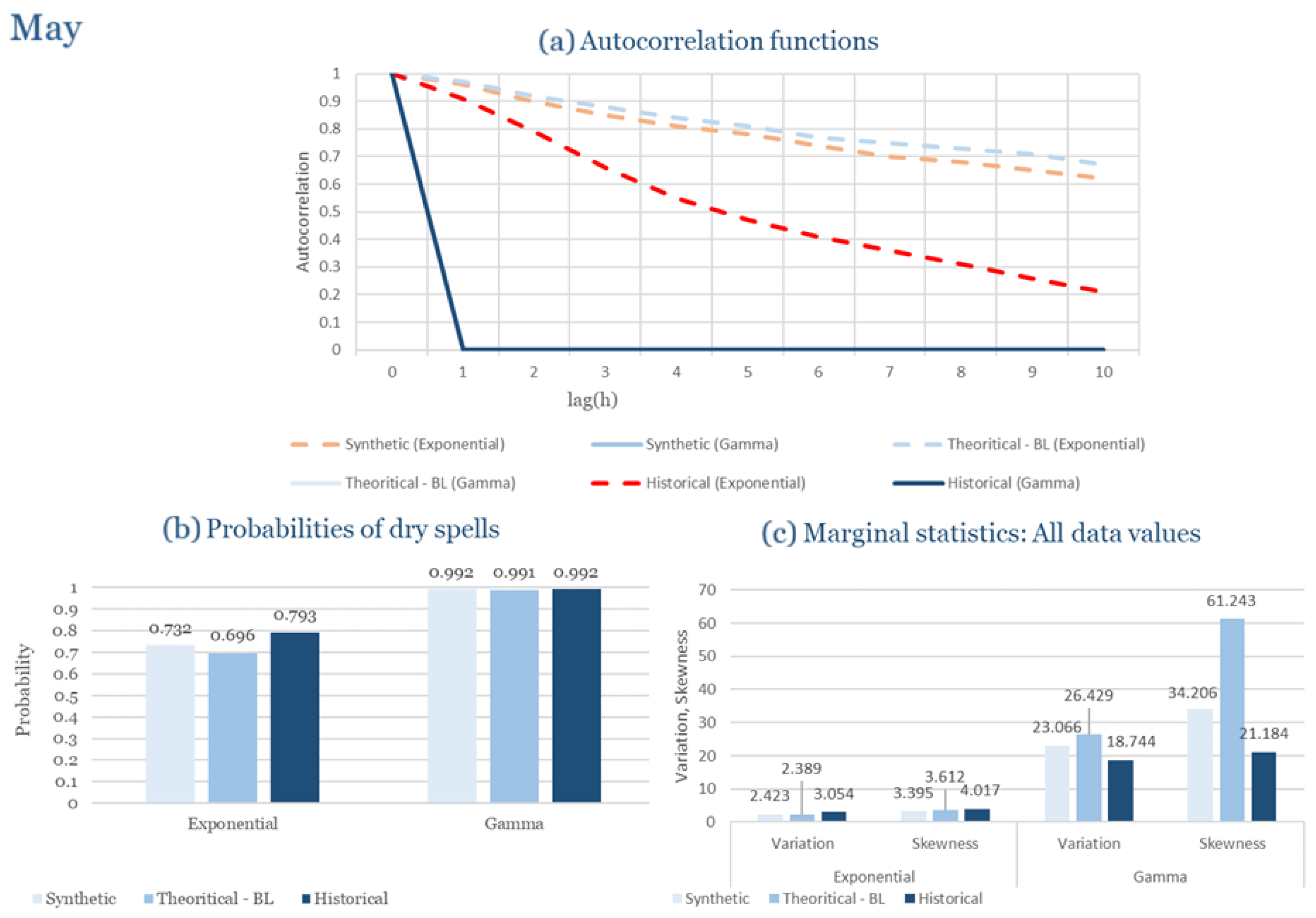
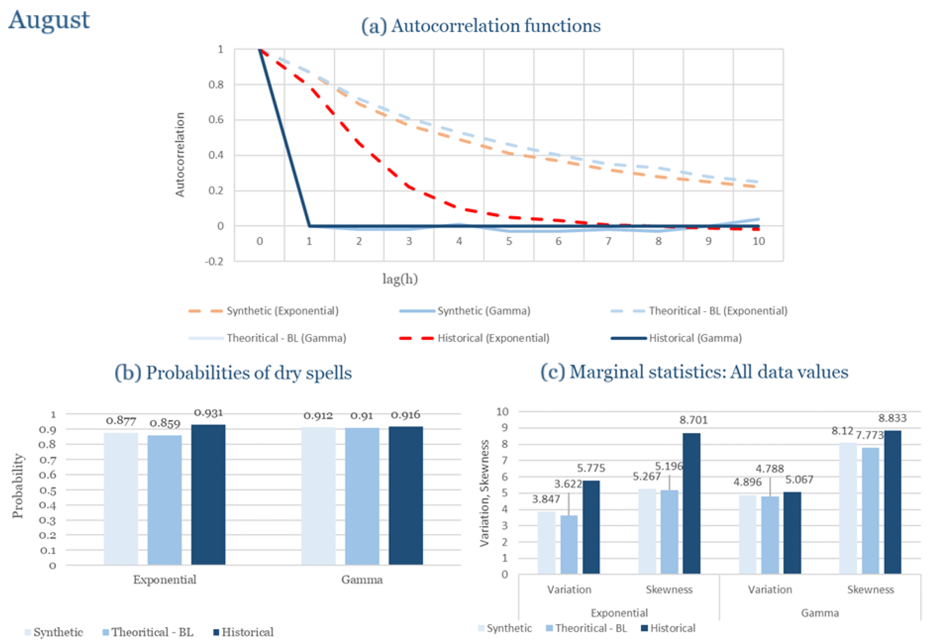
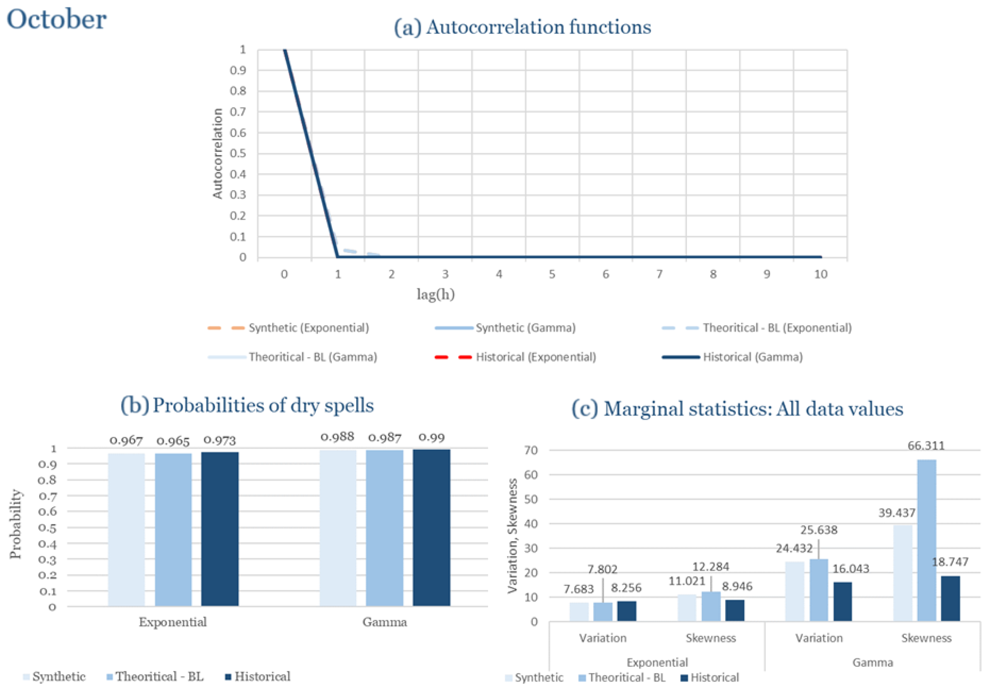
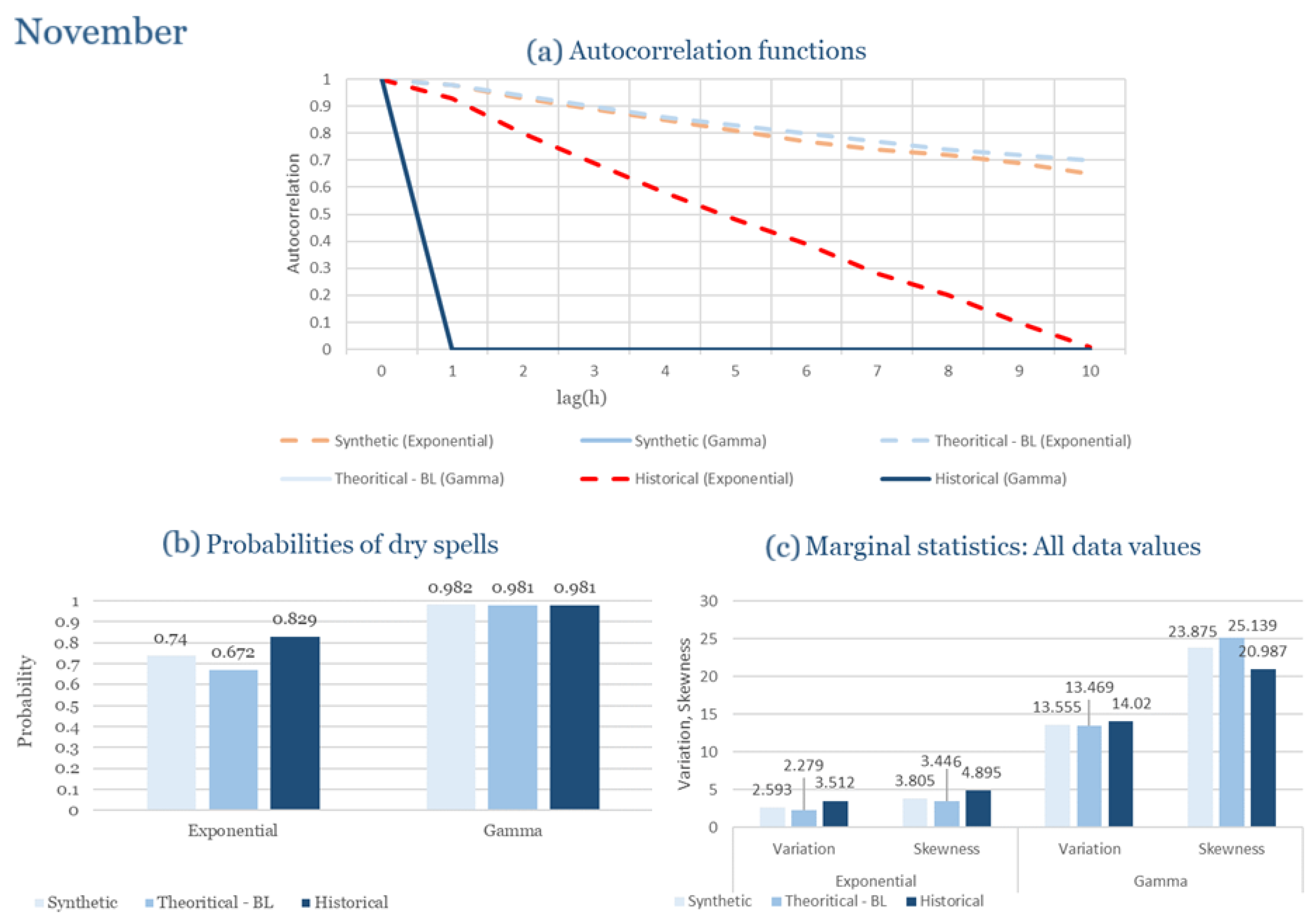
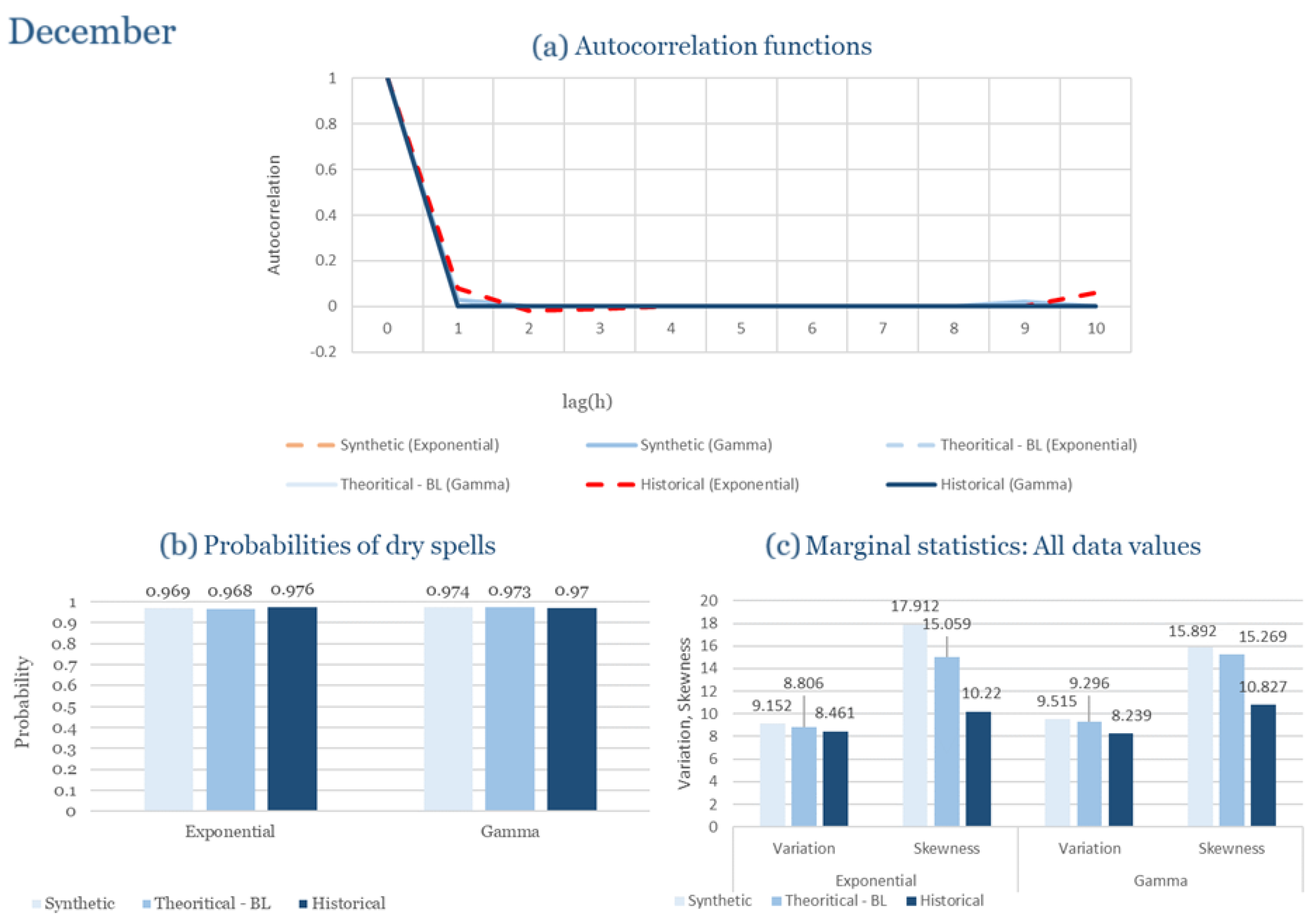
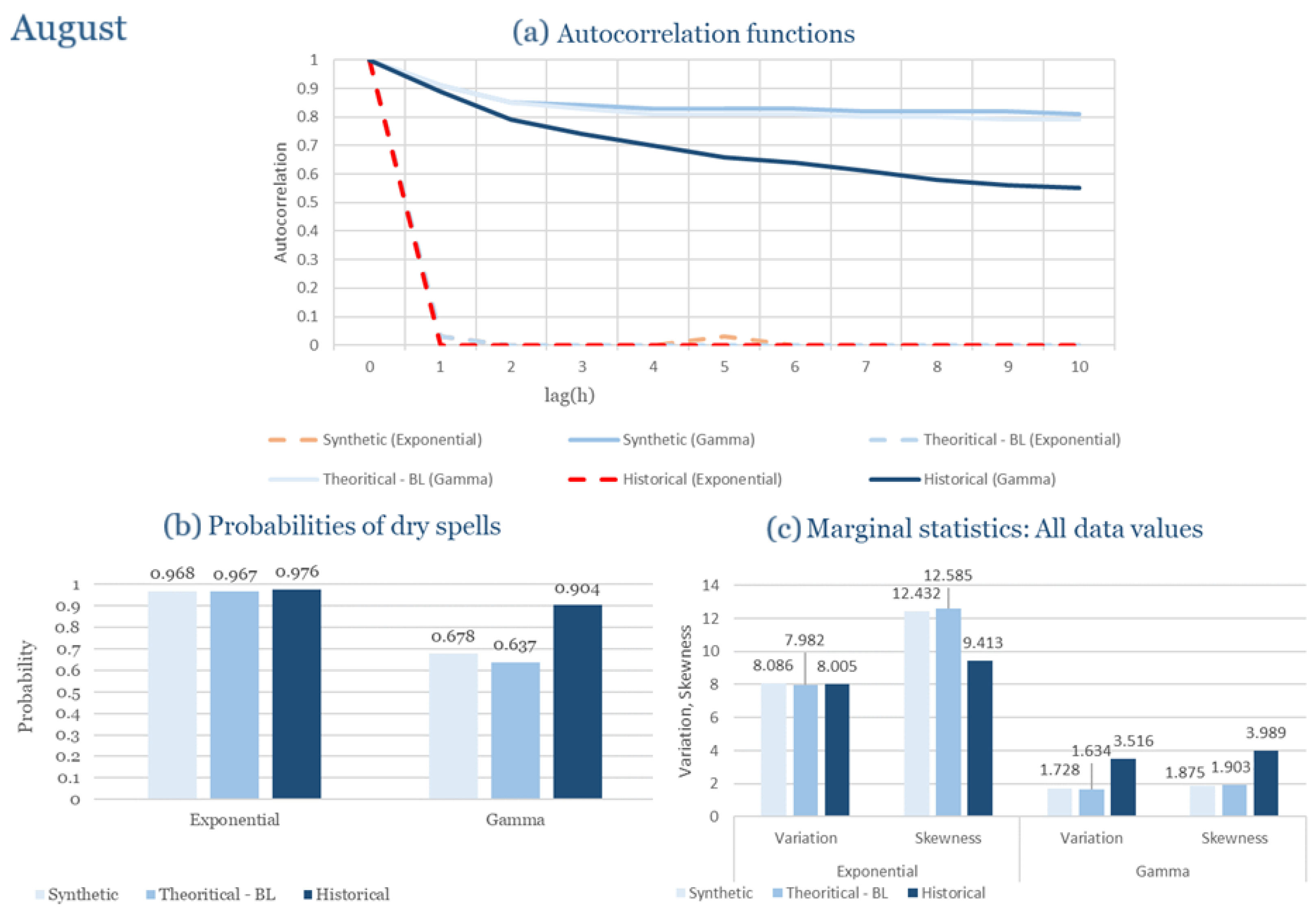
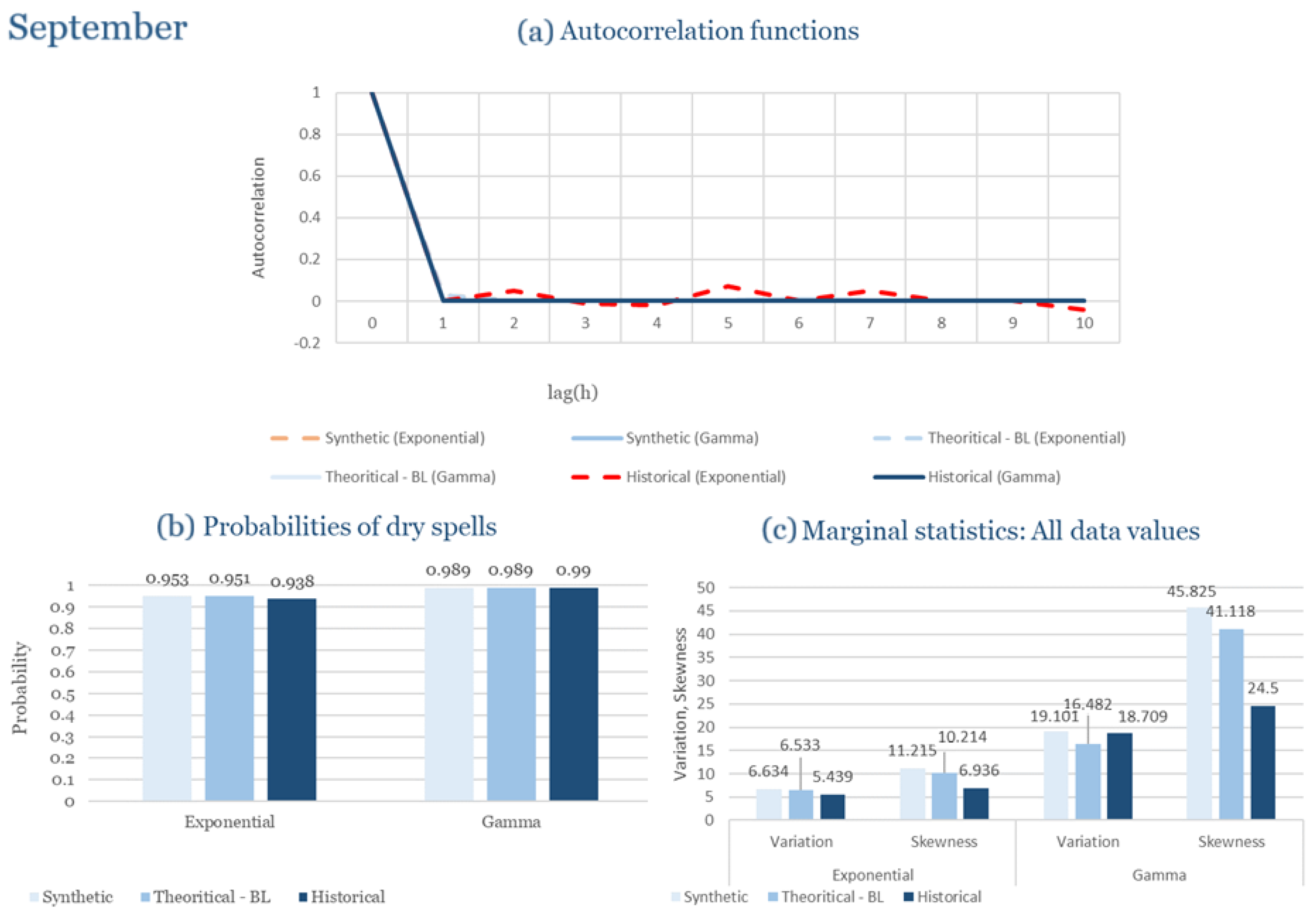
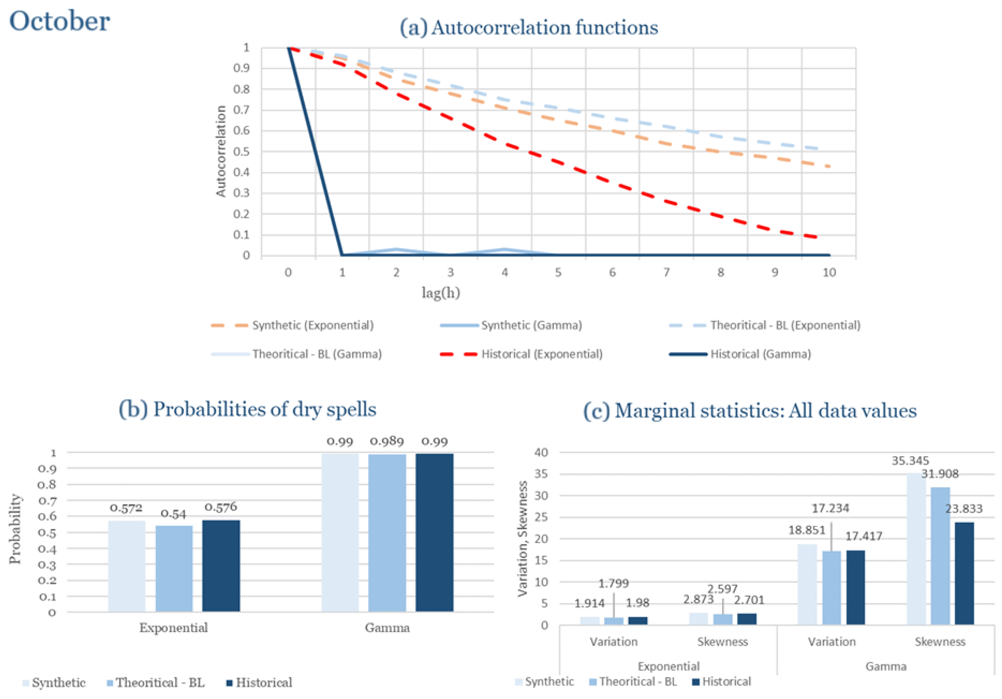
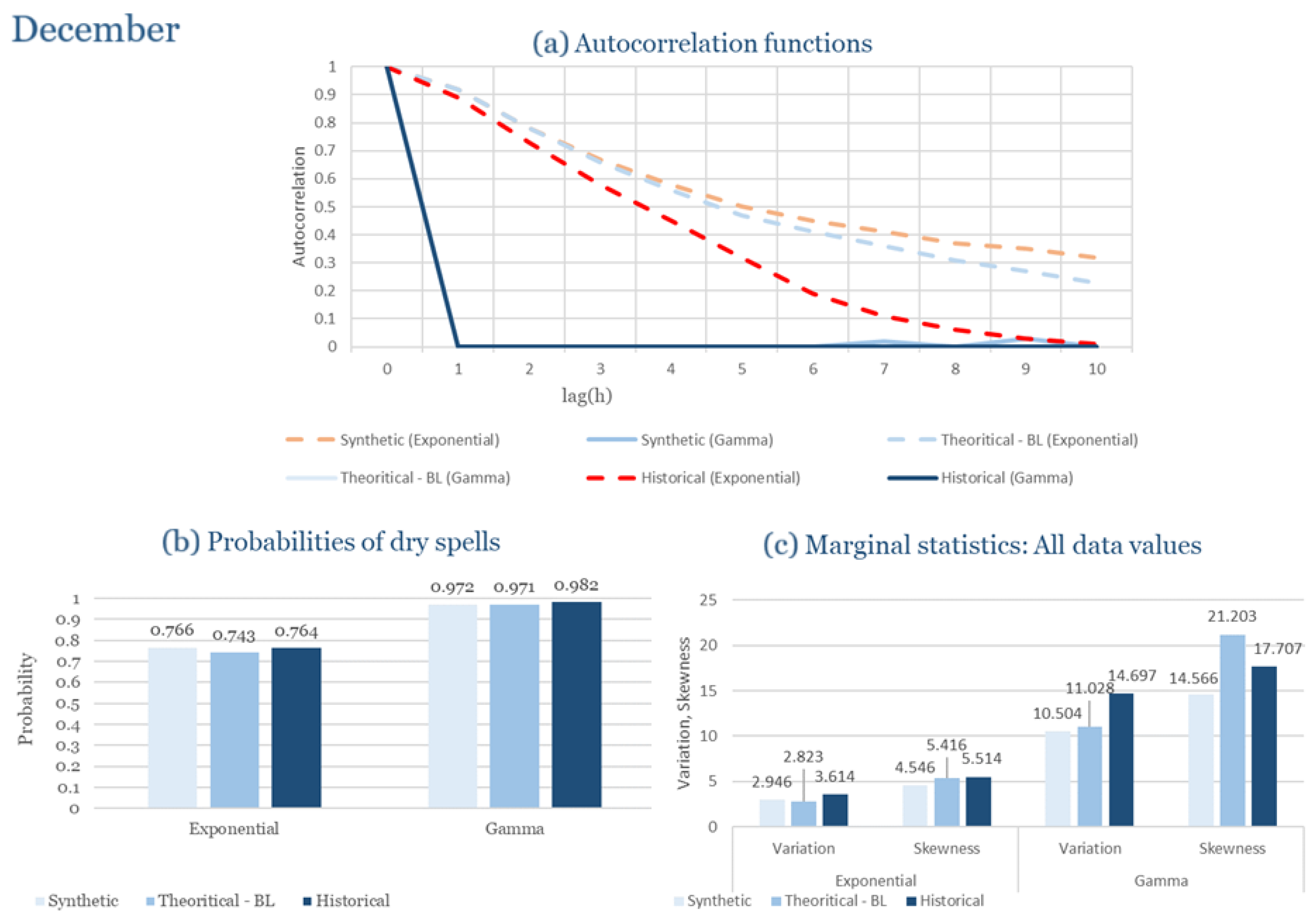
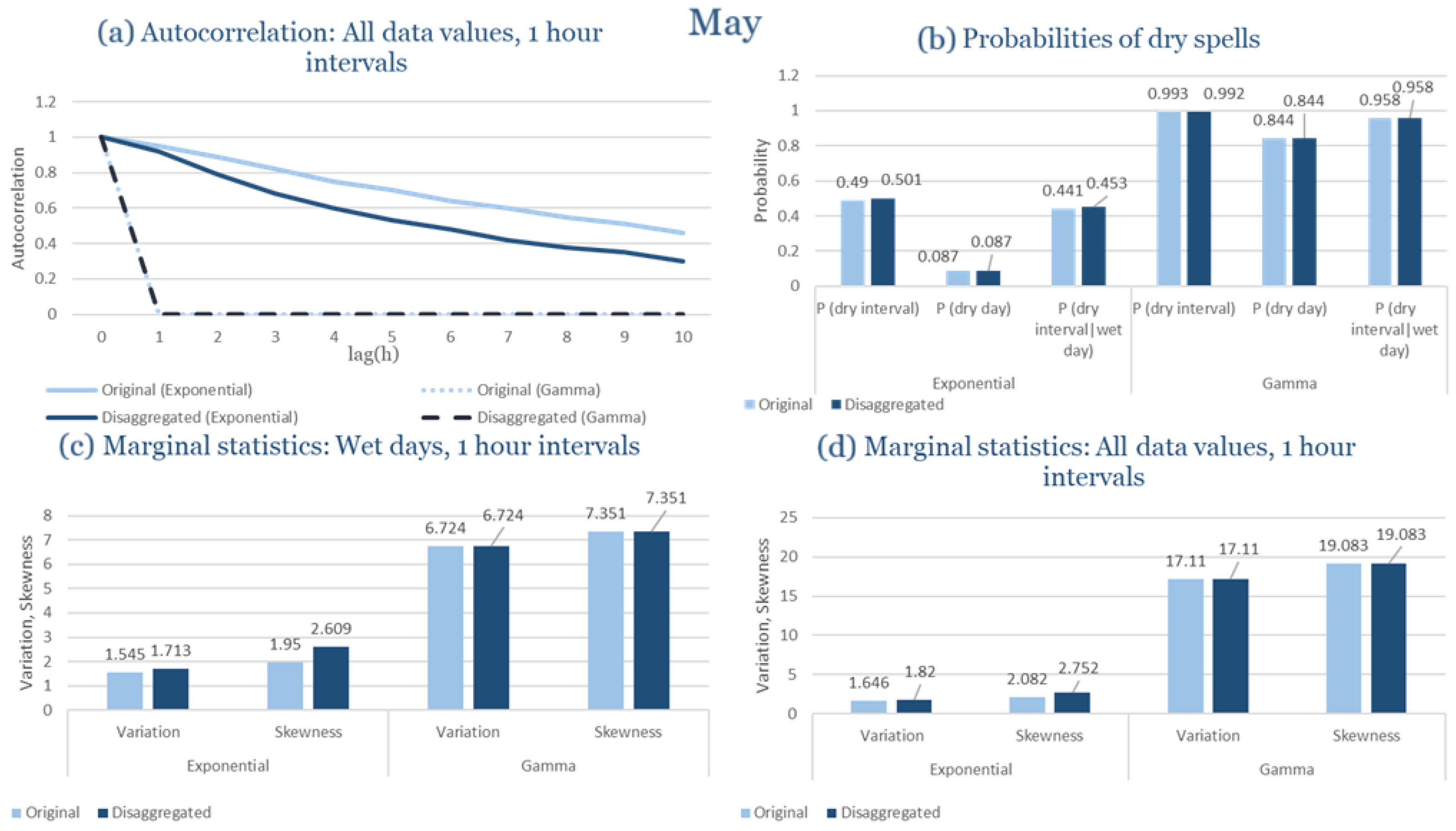
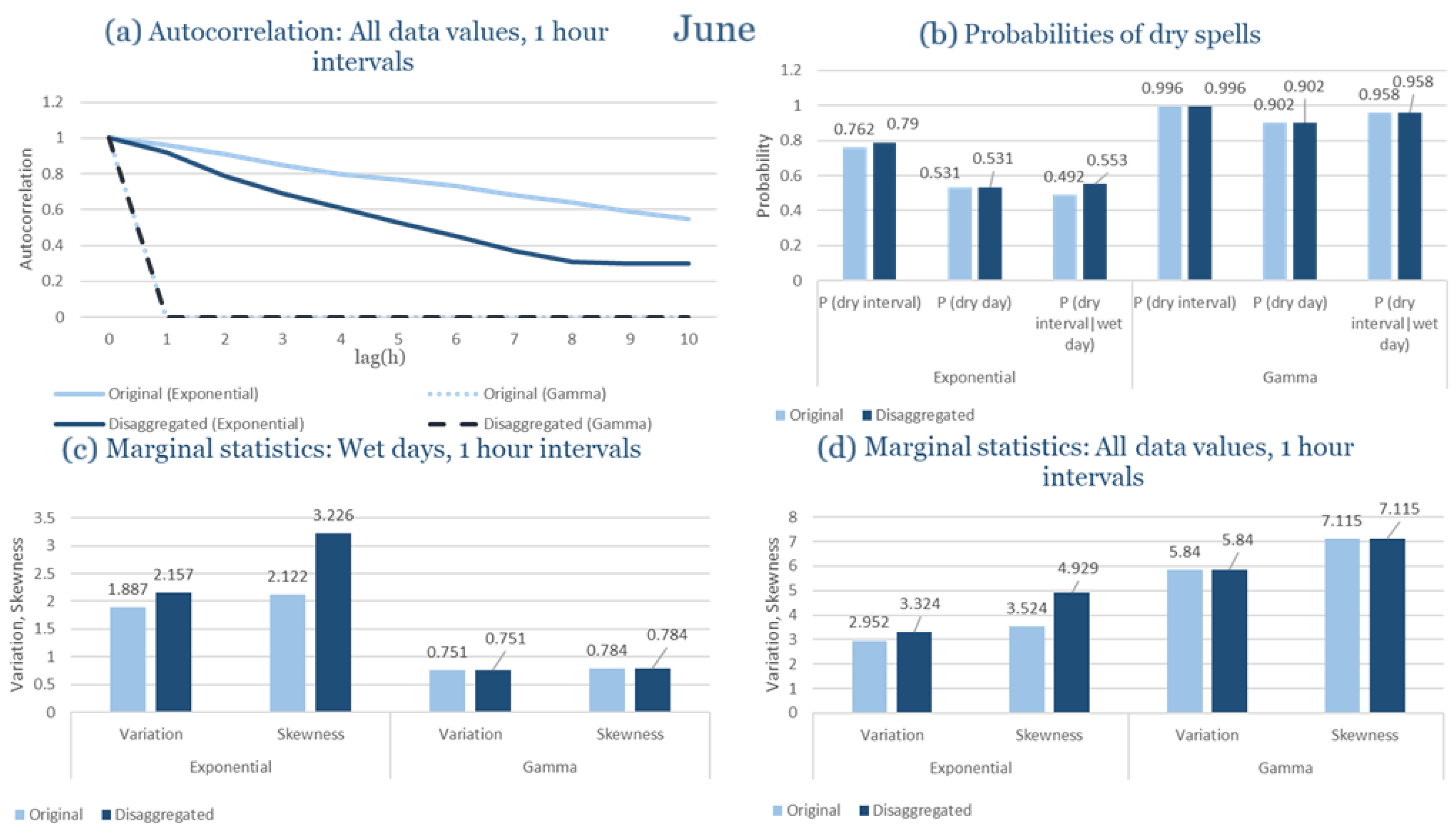
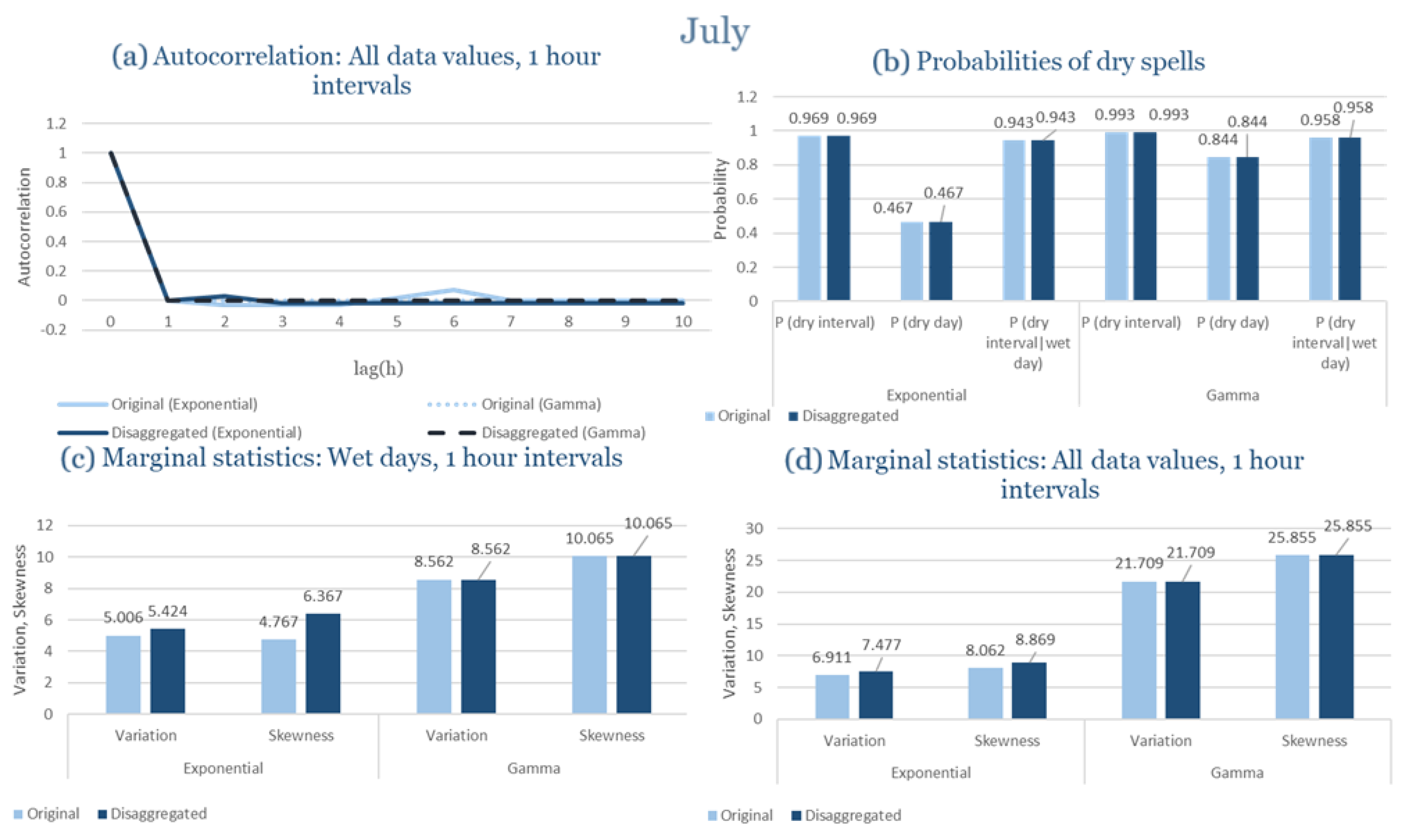
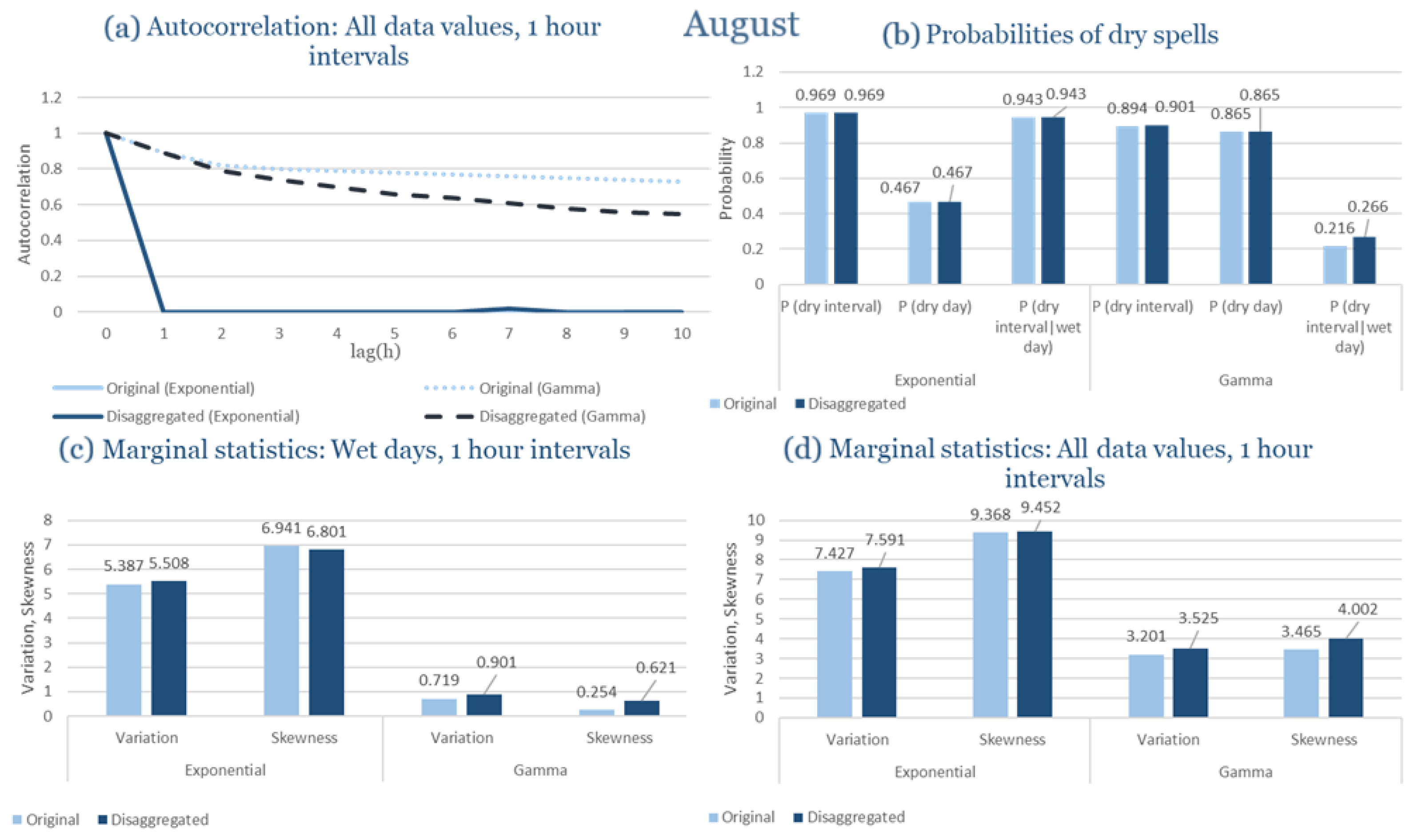
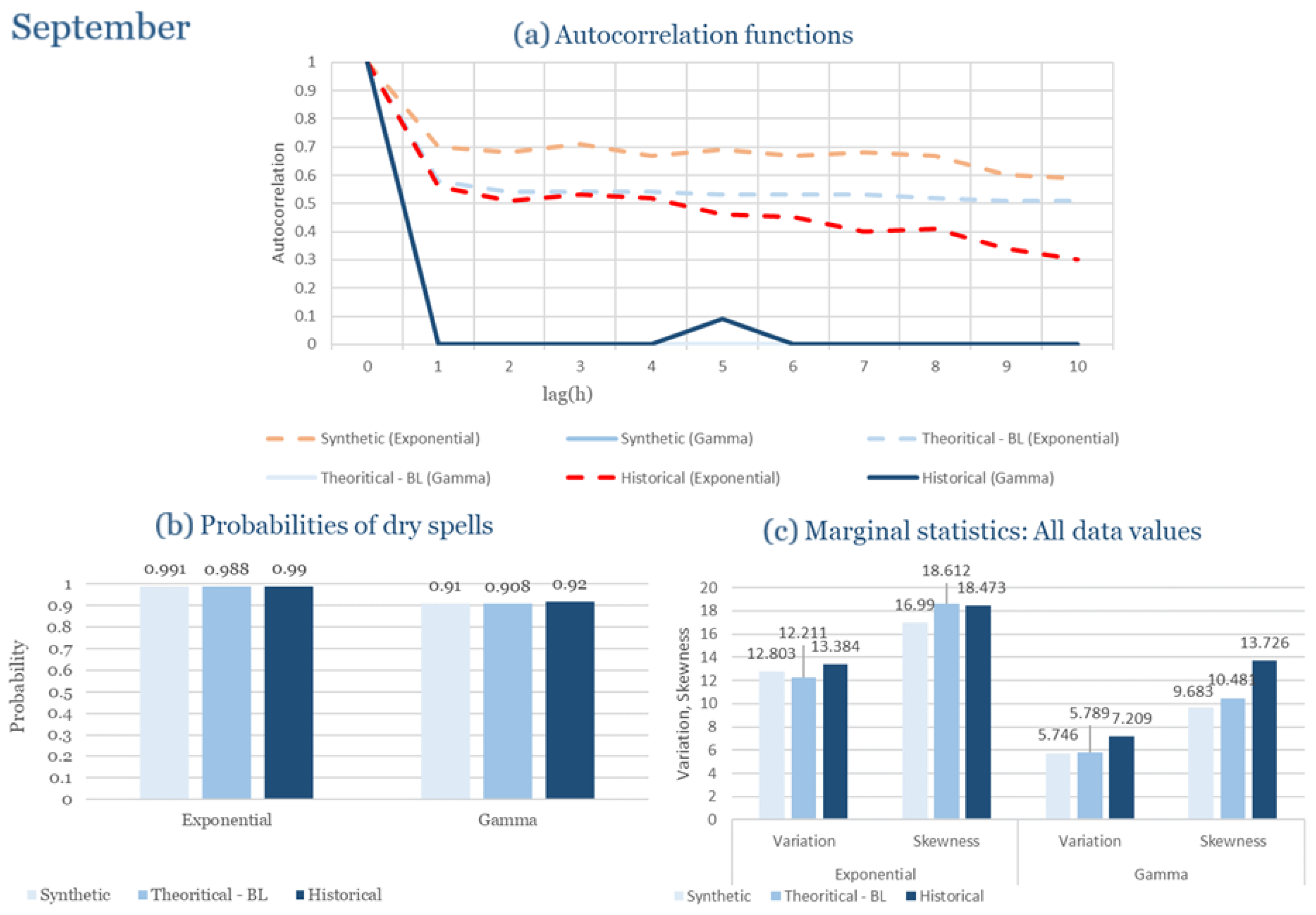
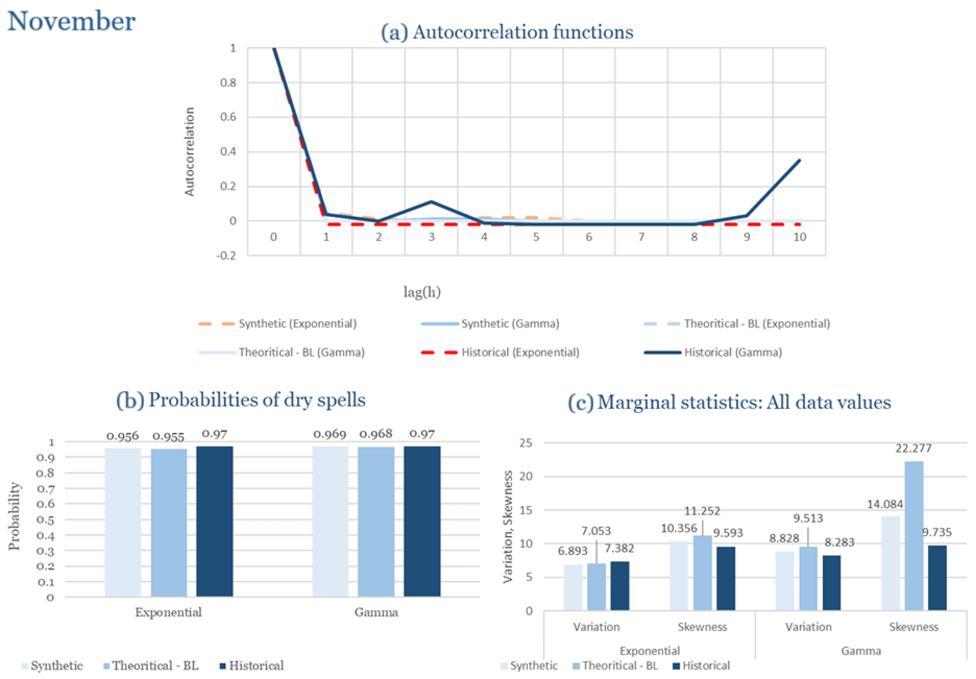
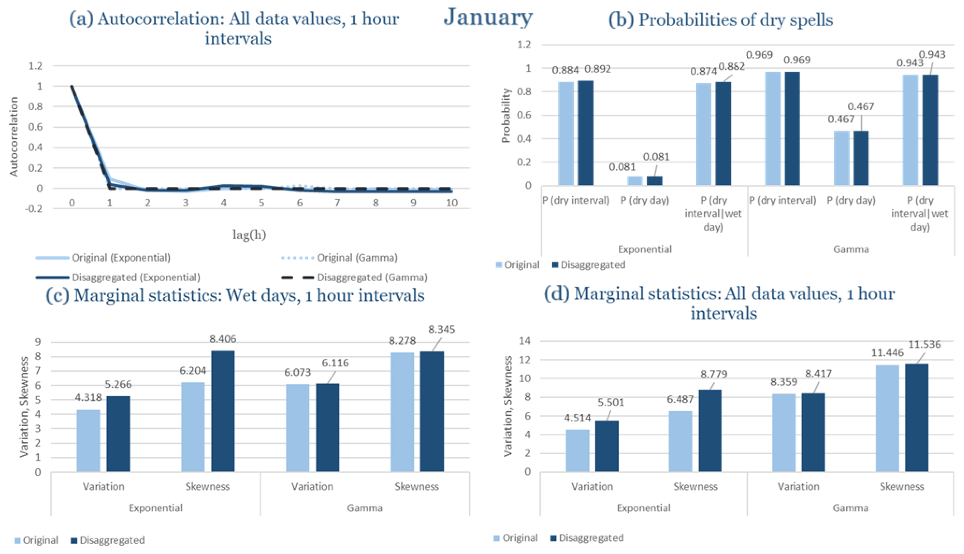
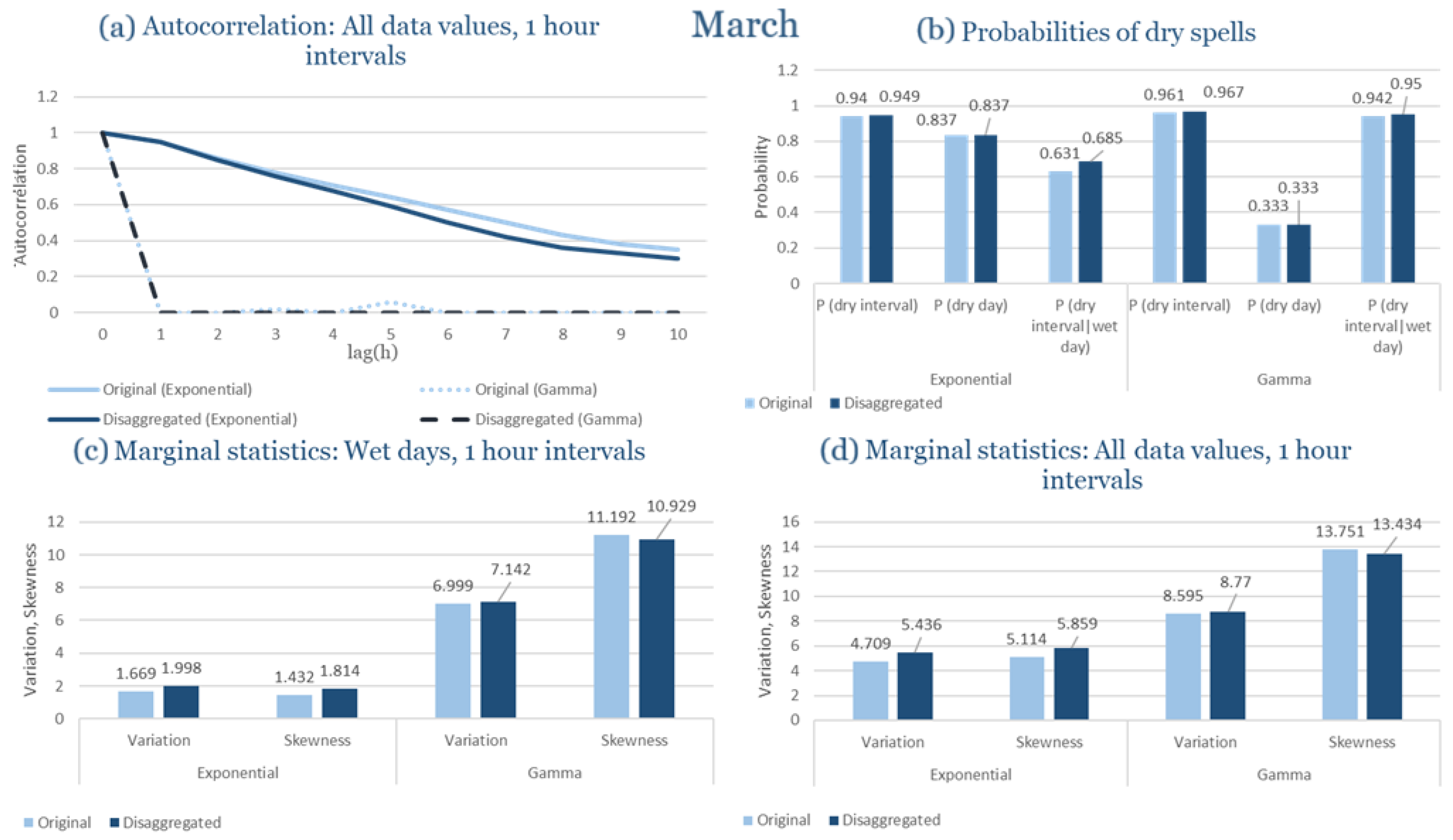
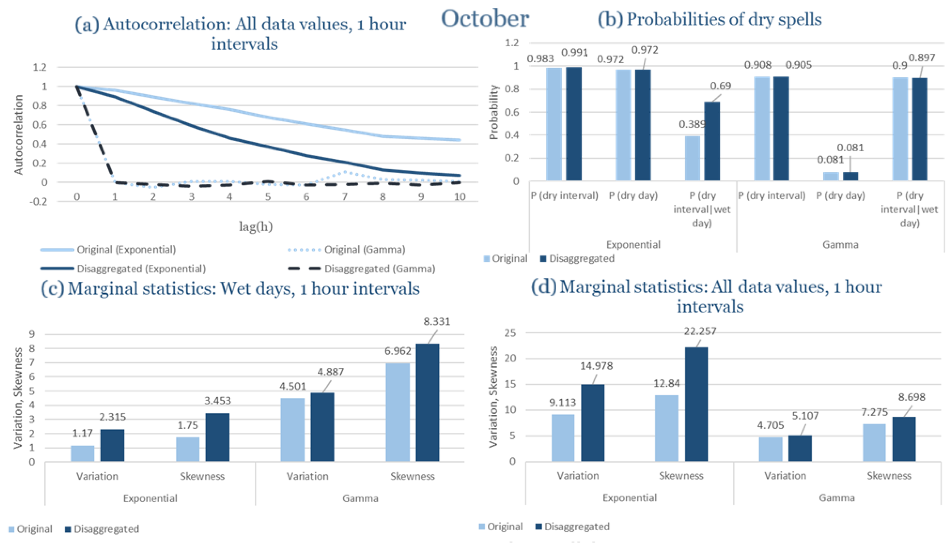
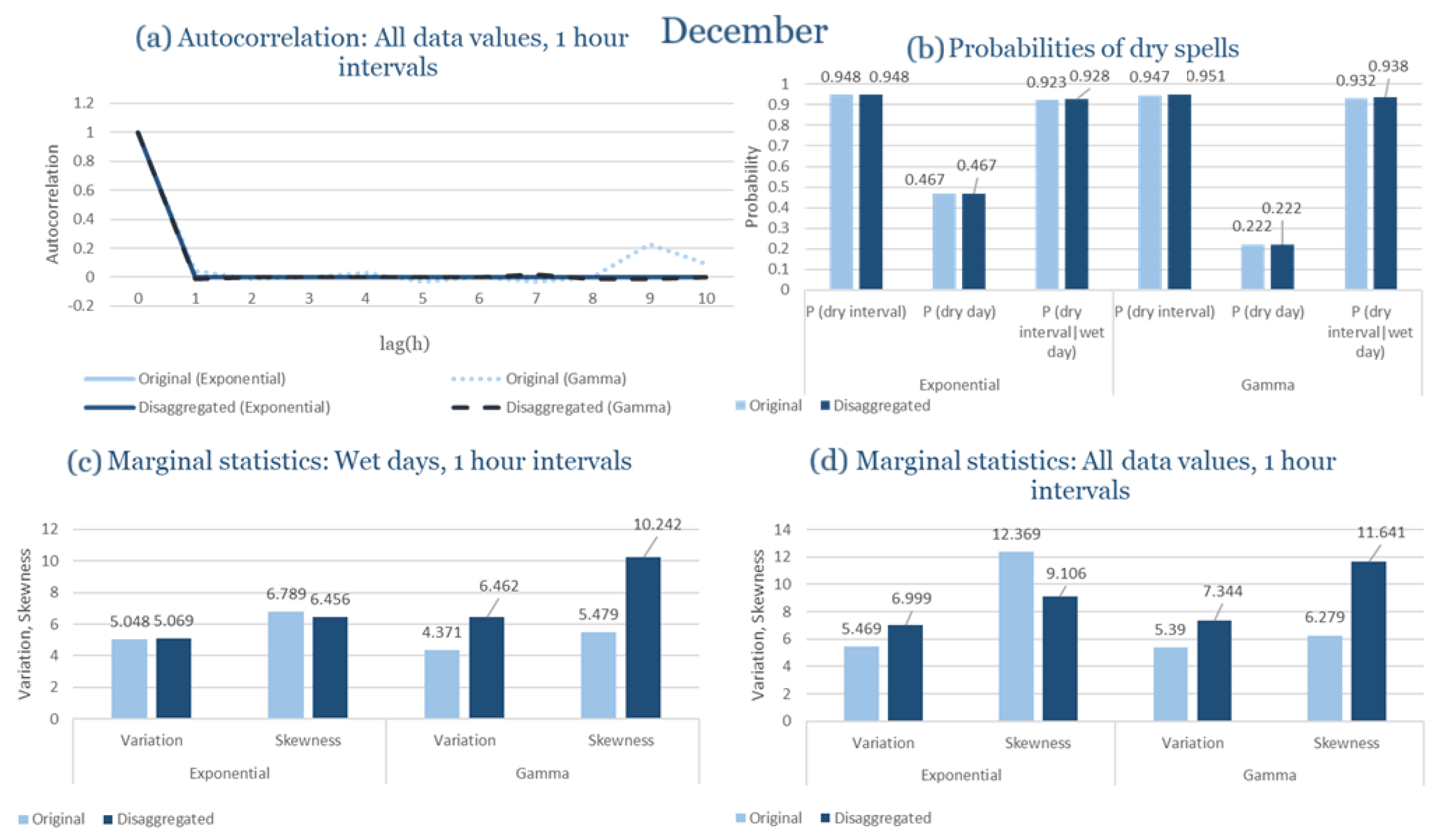
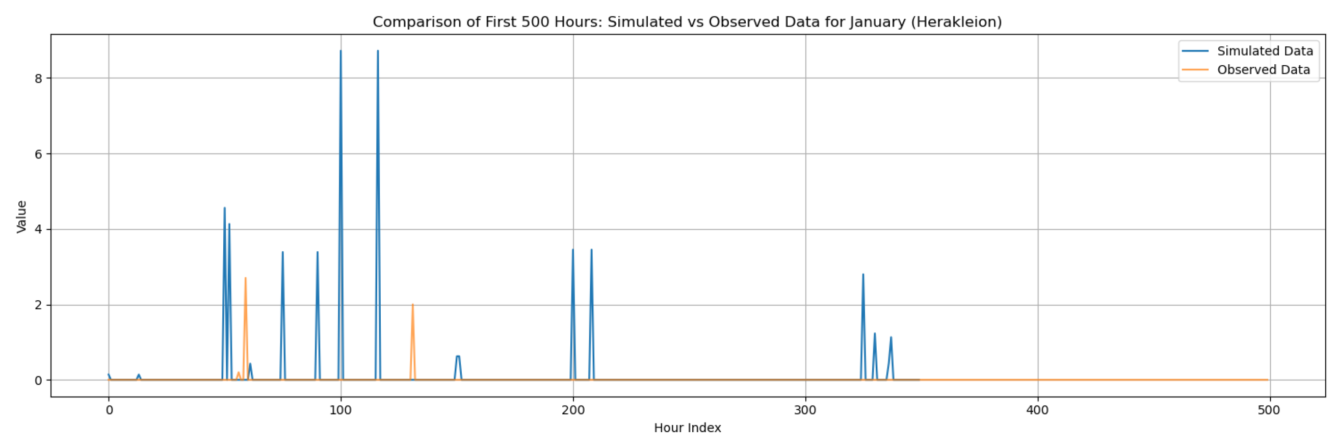
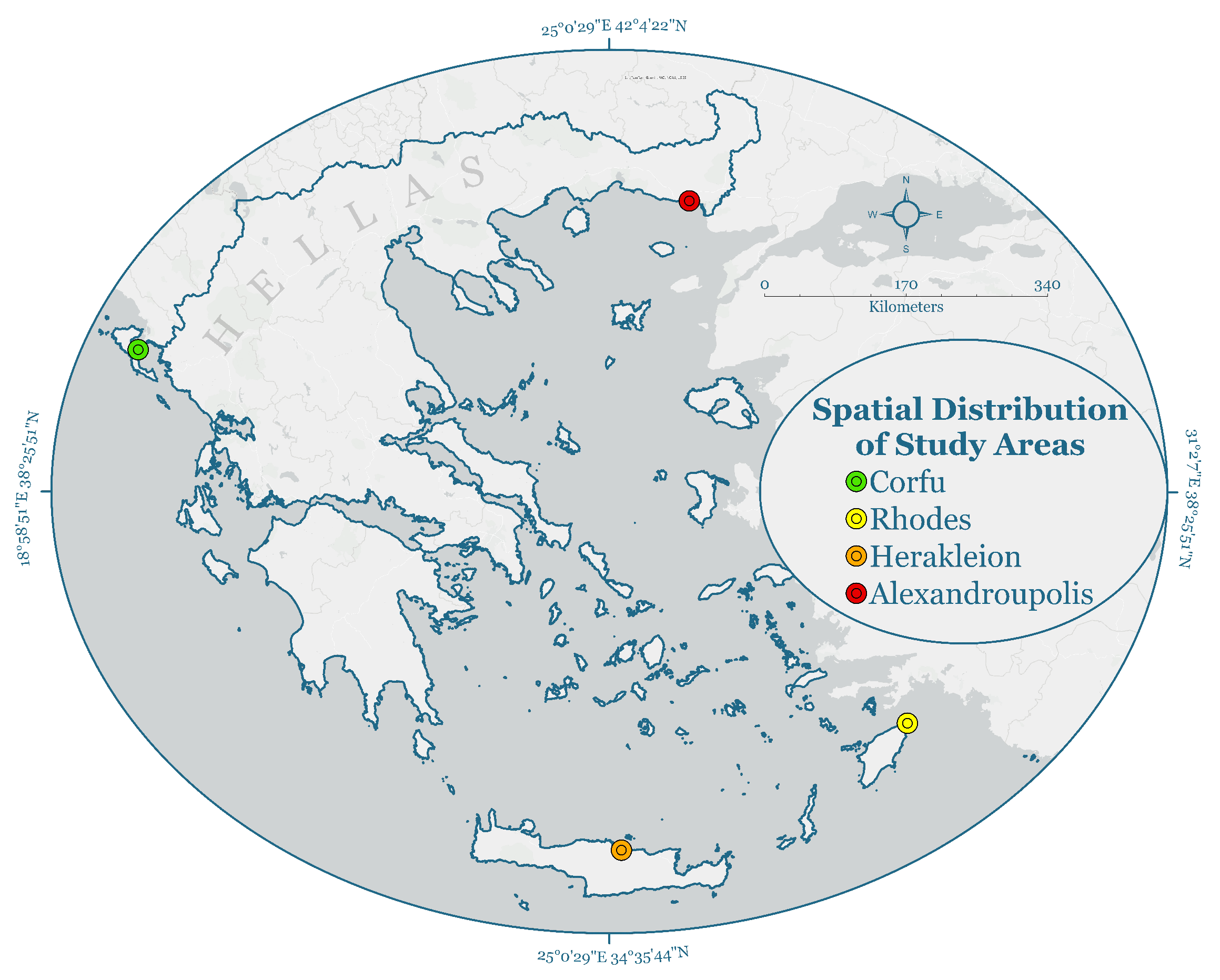
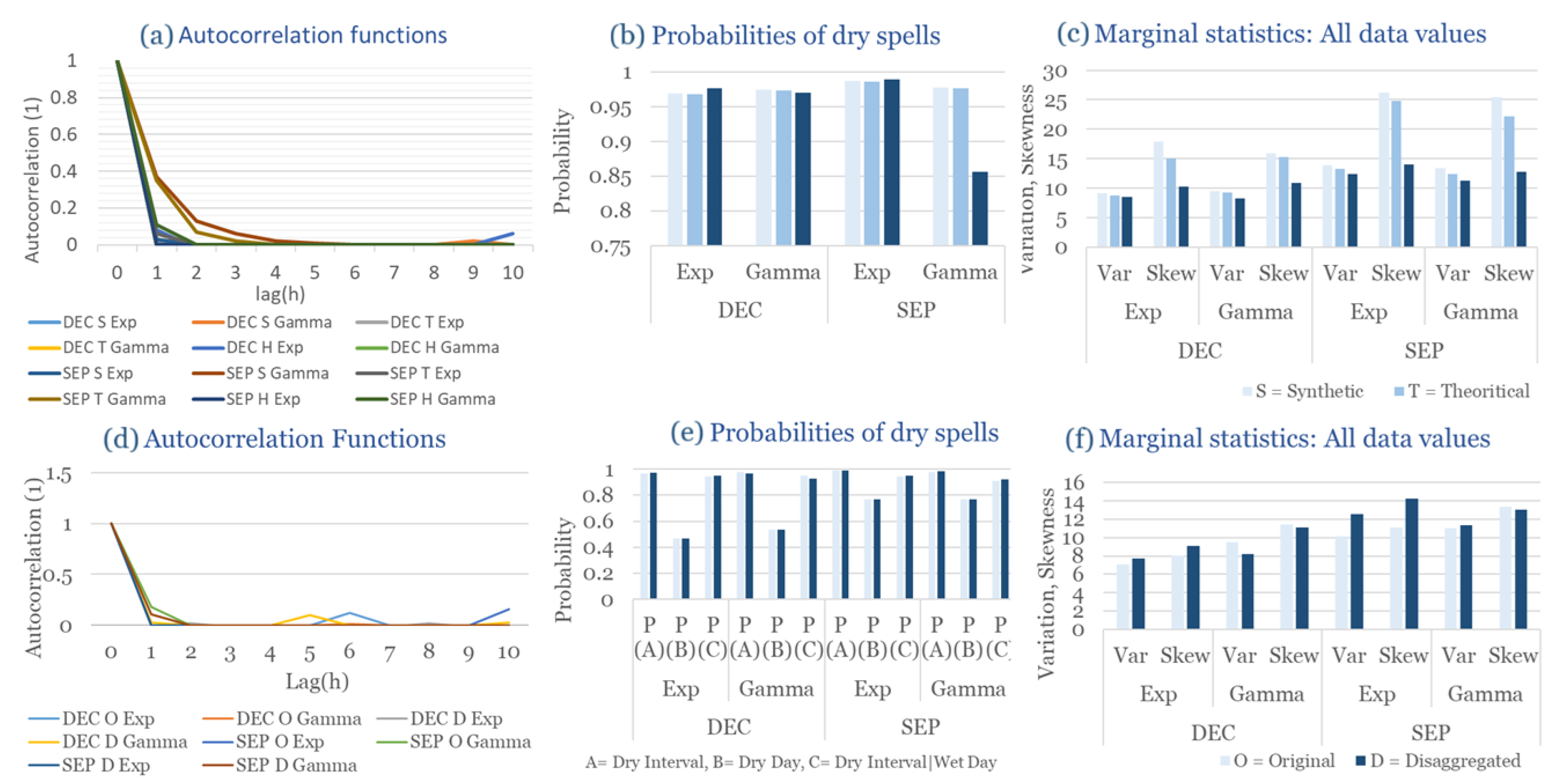
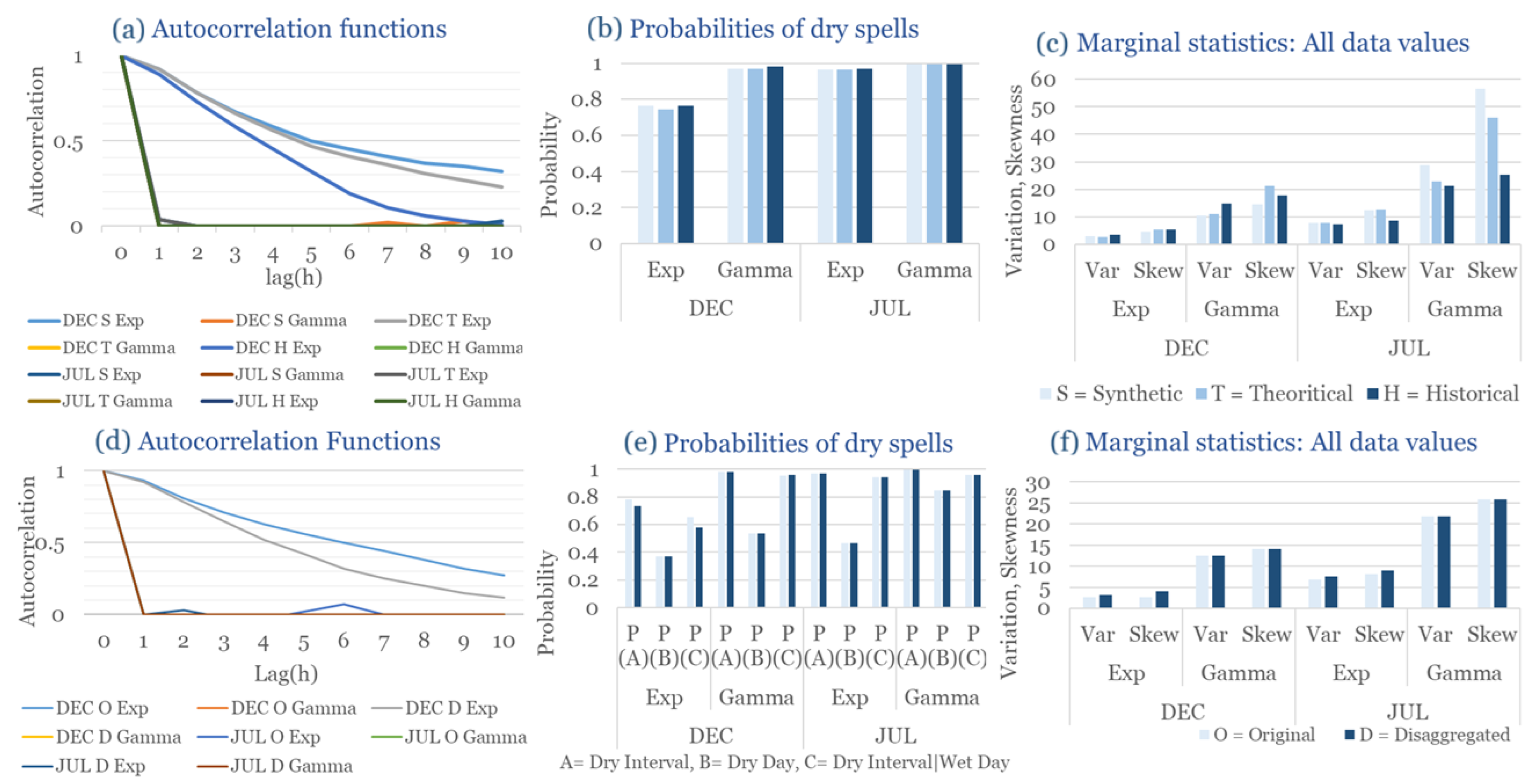
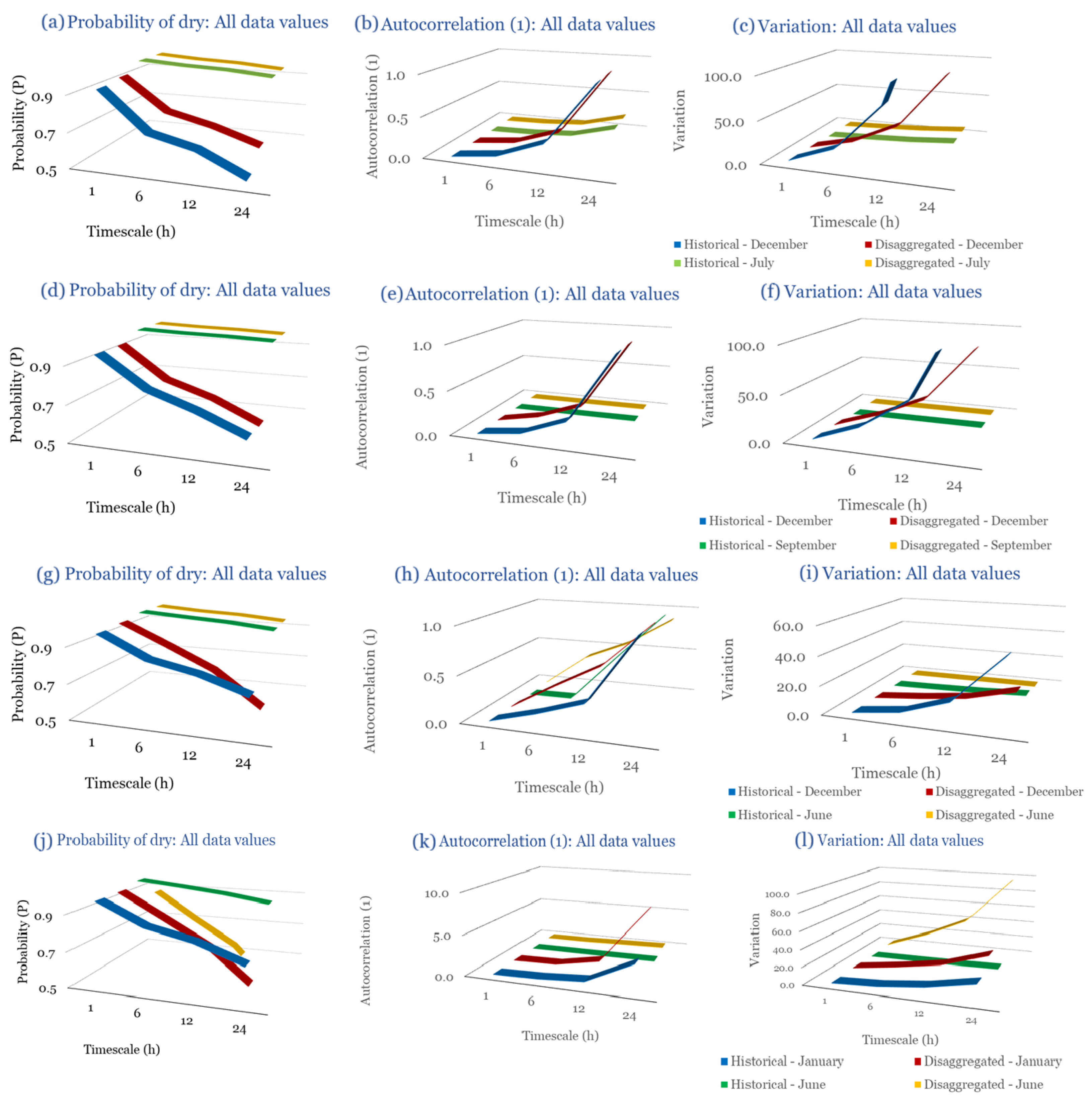
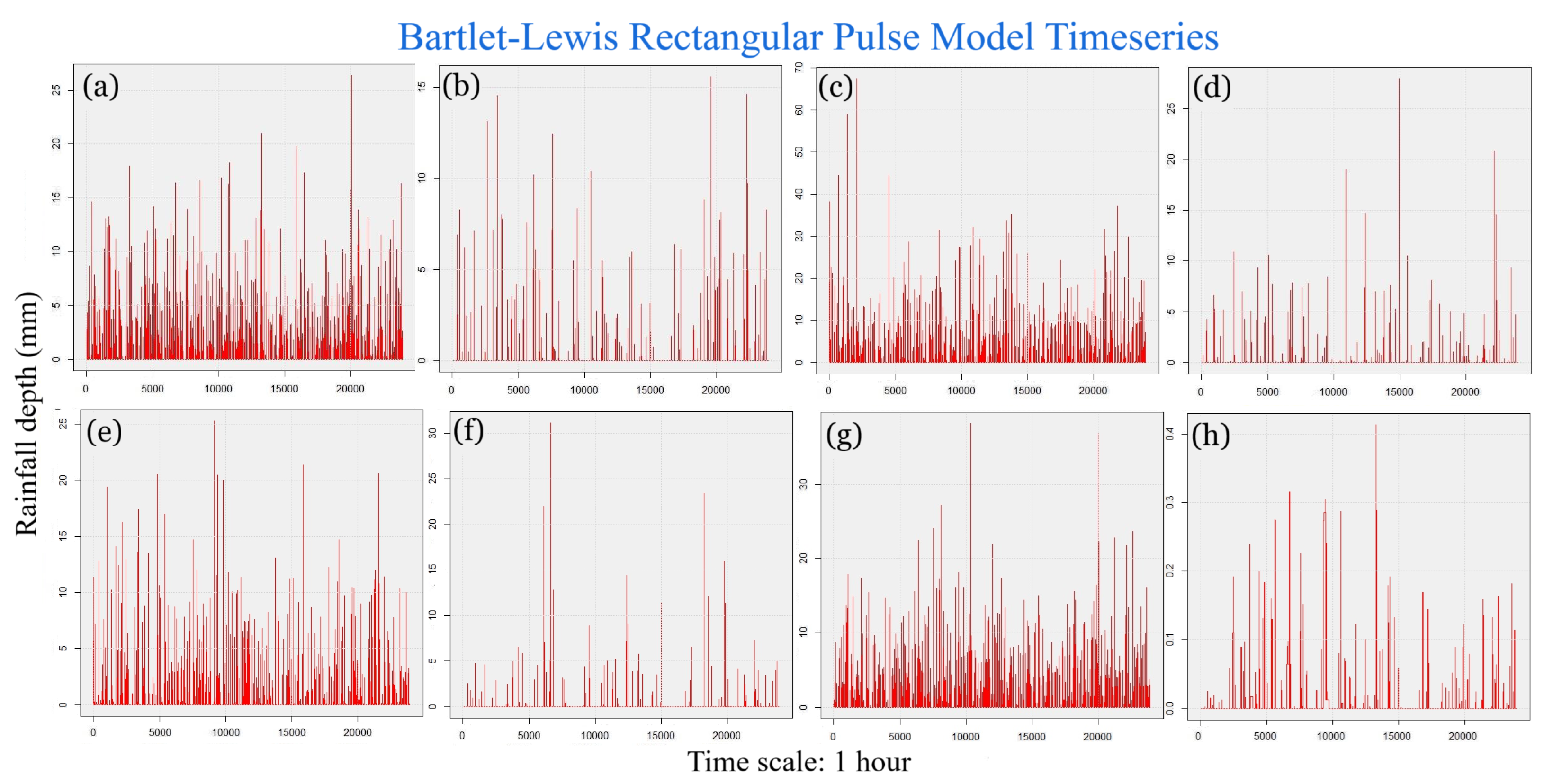
This section contains the complete set of monthly disaggregation results for all four study regions—Corfu, Rhodes, Alexandroupolis, and Herakleion—using both exponential and gamma pulse intensity distributions. While the main manuscript presents results only for the wettest and driest months of each region to emphasize key contrasts, the full twelve-month comparisons are provided here to ensure transparency and reproducibility. The figures include statistical comparisons between observed and synthetic rainfall series, supporting the evaluation of the RBLRPM’s performance across different climatic conditions and seasonal regimes.
Figure A1.
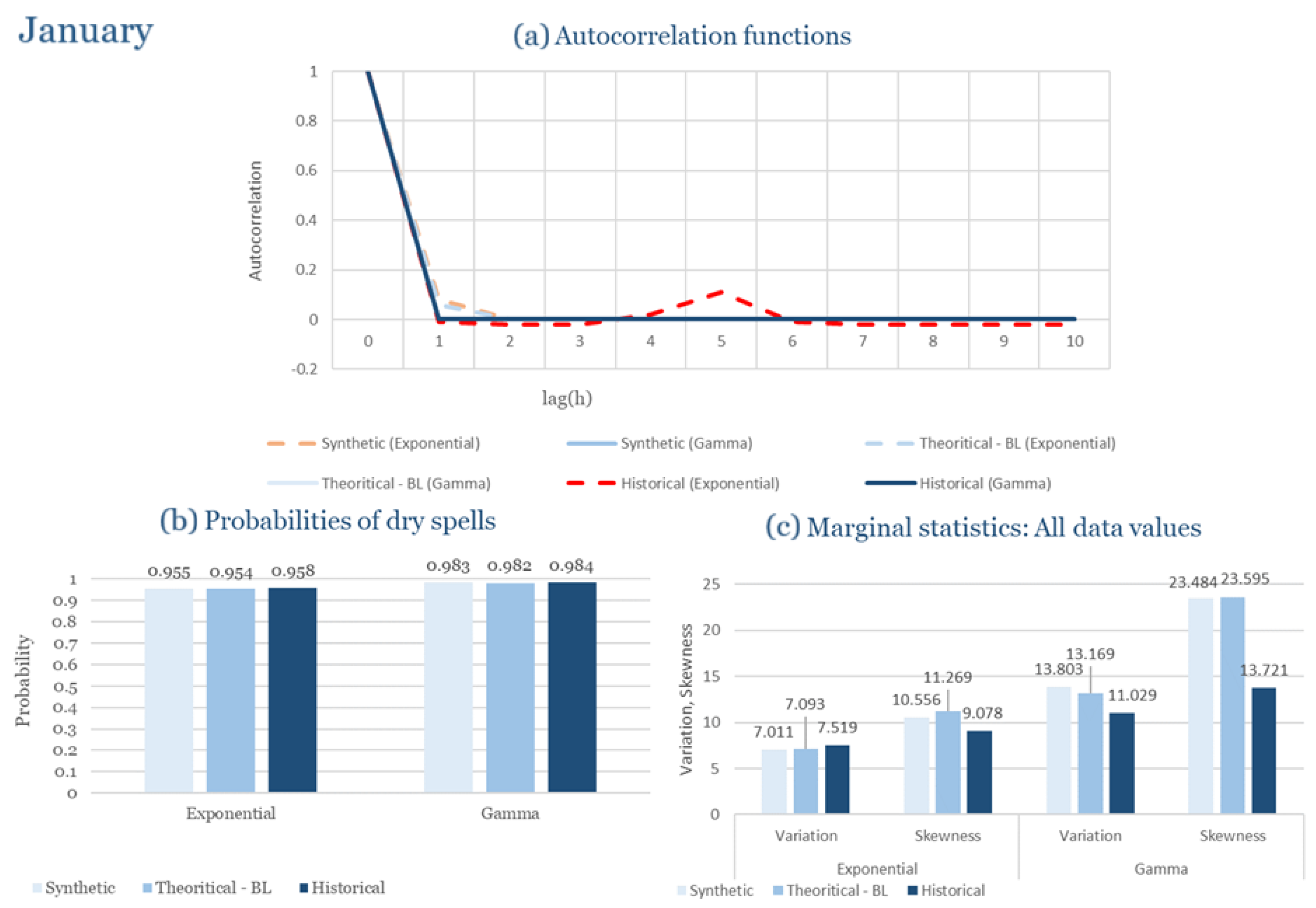
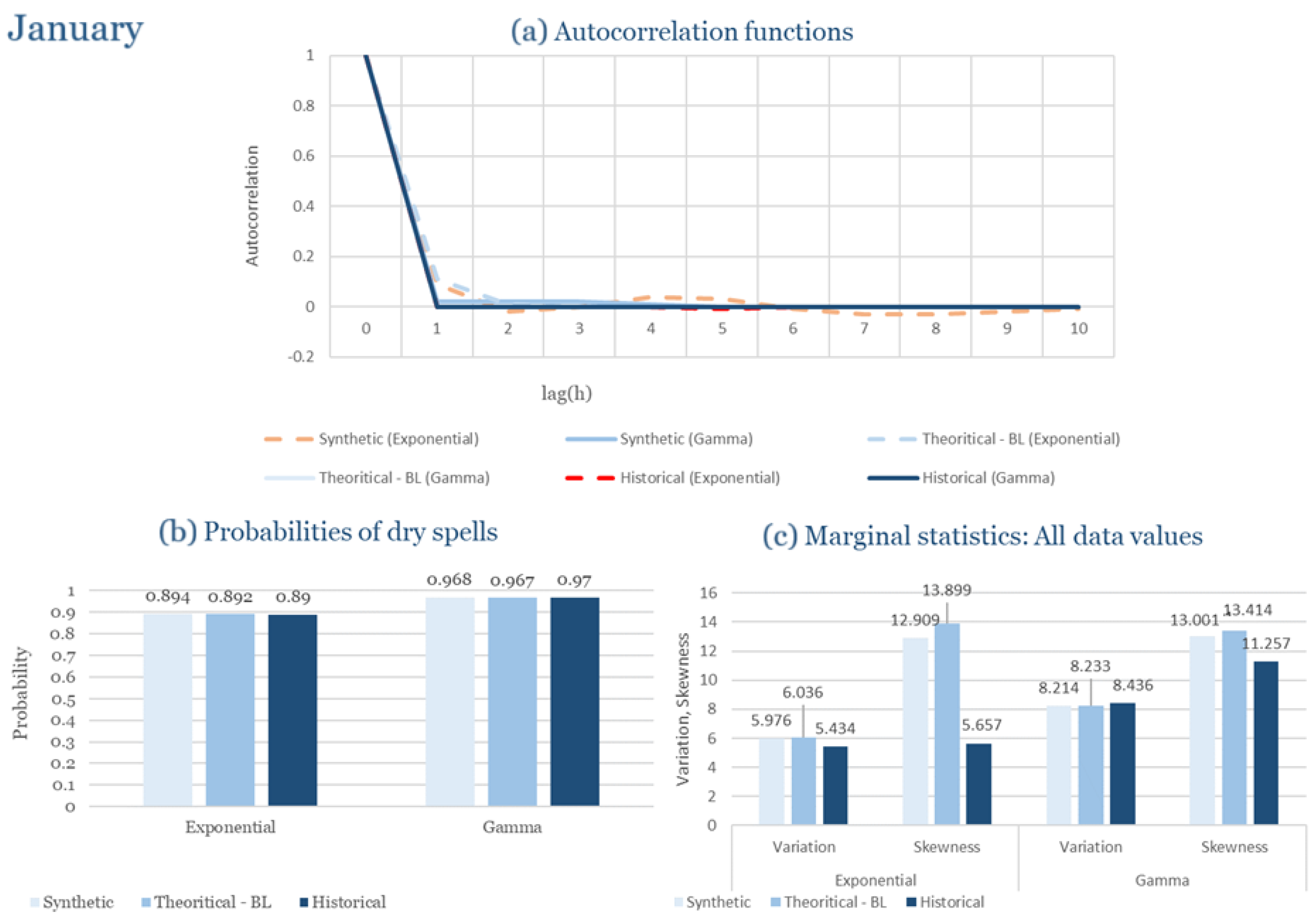
Statistical Characteristics of Corfu for January, with the intensity of the pulses following both distributions, where: (a) the diagram of the autocorrelation coefficient, (b) the diagram of the probability of dry and (c) the diagrams for the coefficient of variation and skewness of the historical and synthetic timeseries.
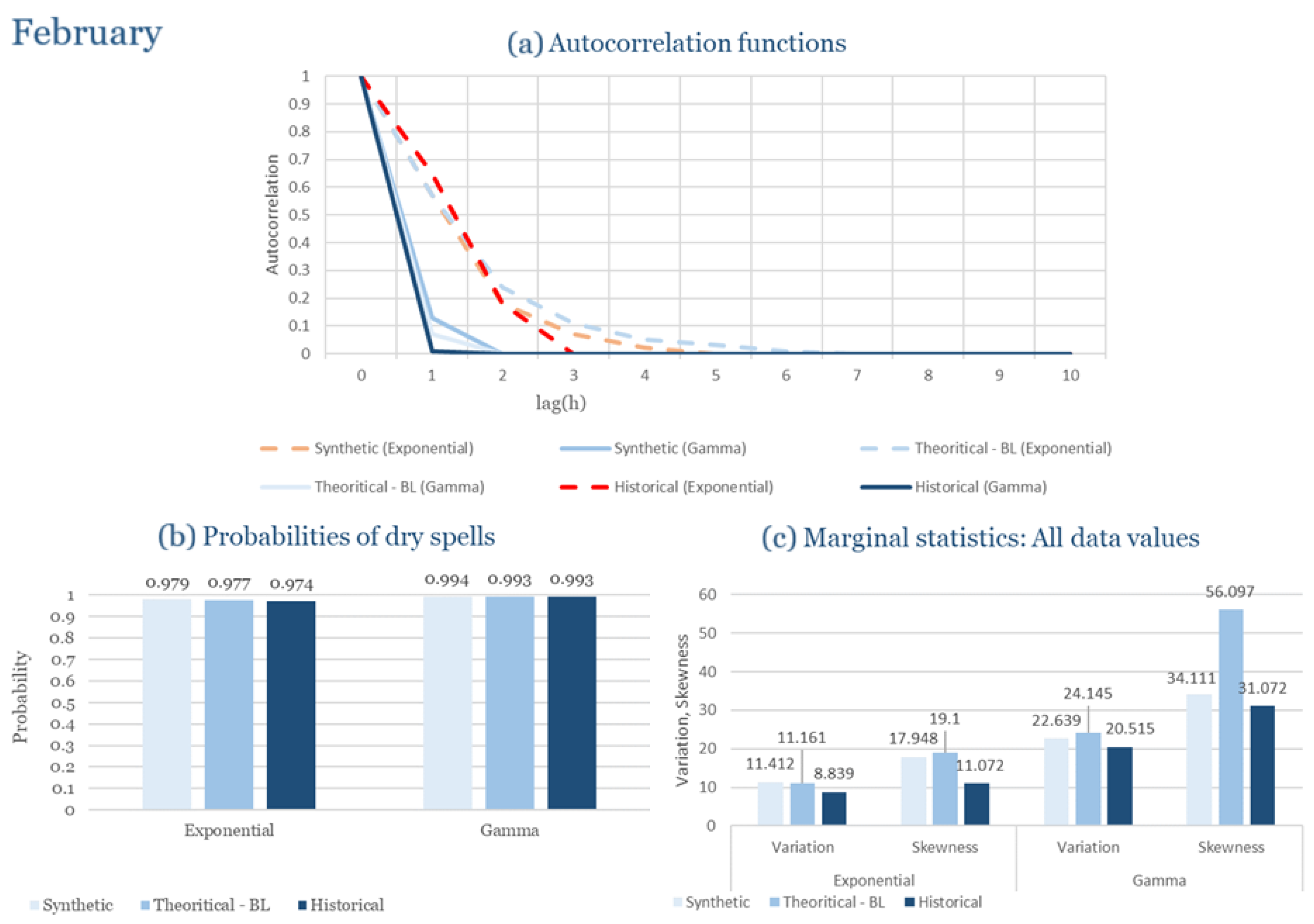
Figure A2.
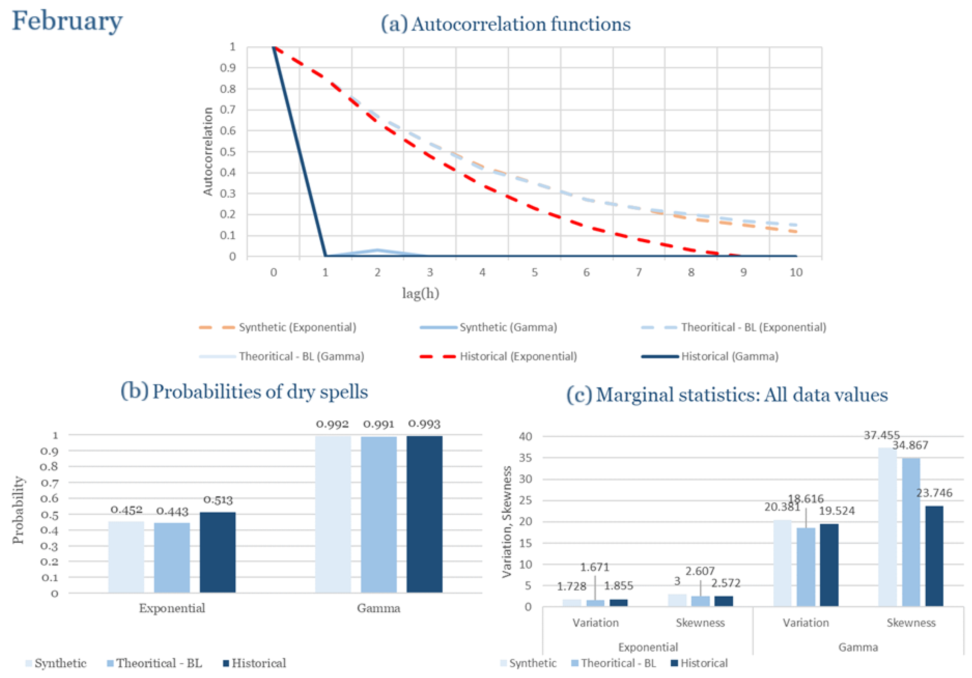
Statistical Characteristics of Corfu for February, with the intensity of the pulses following both distributions, where: (a) the diagram of the autocorrelation coefficient, (b) the diagram of the probability of dry and (c) the diagrams for the coefficient of variation and skewness of the historical and synthetic timeseries.
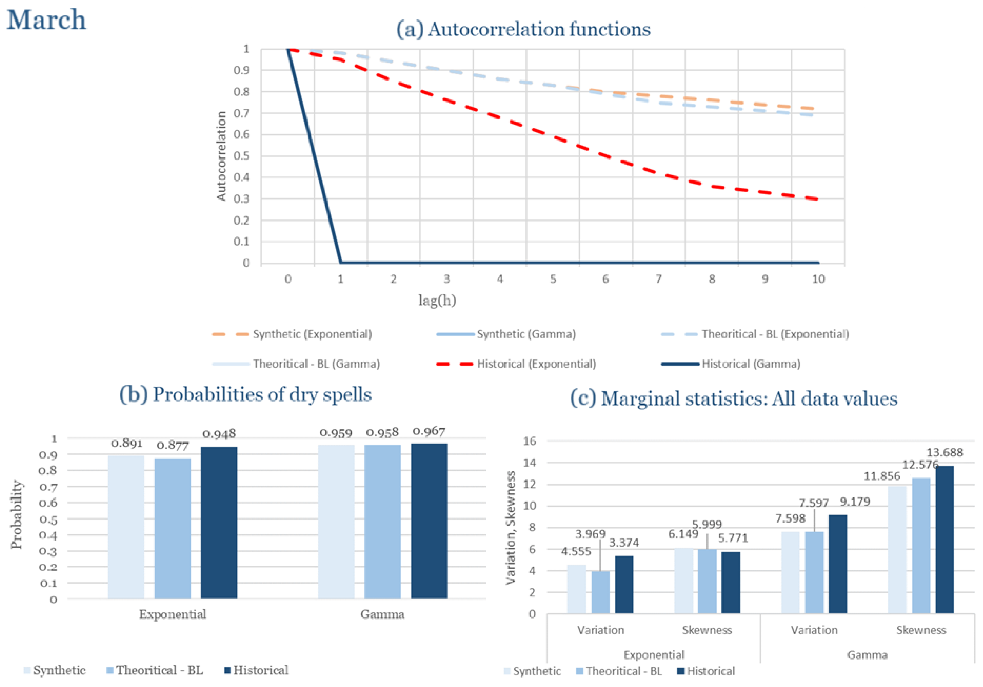
Figure A3.
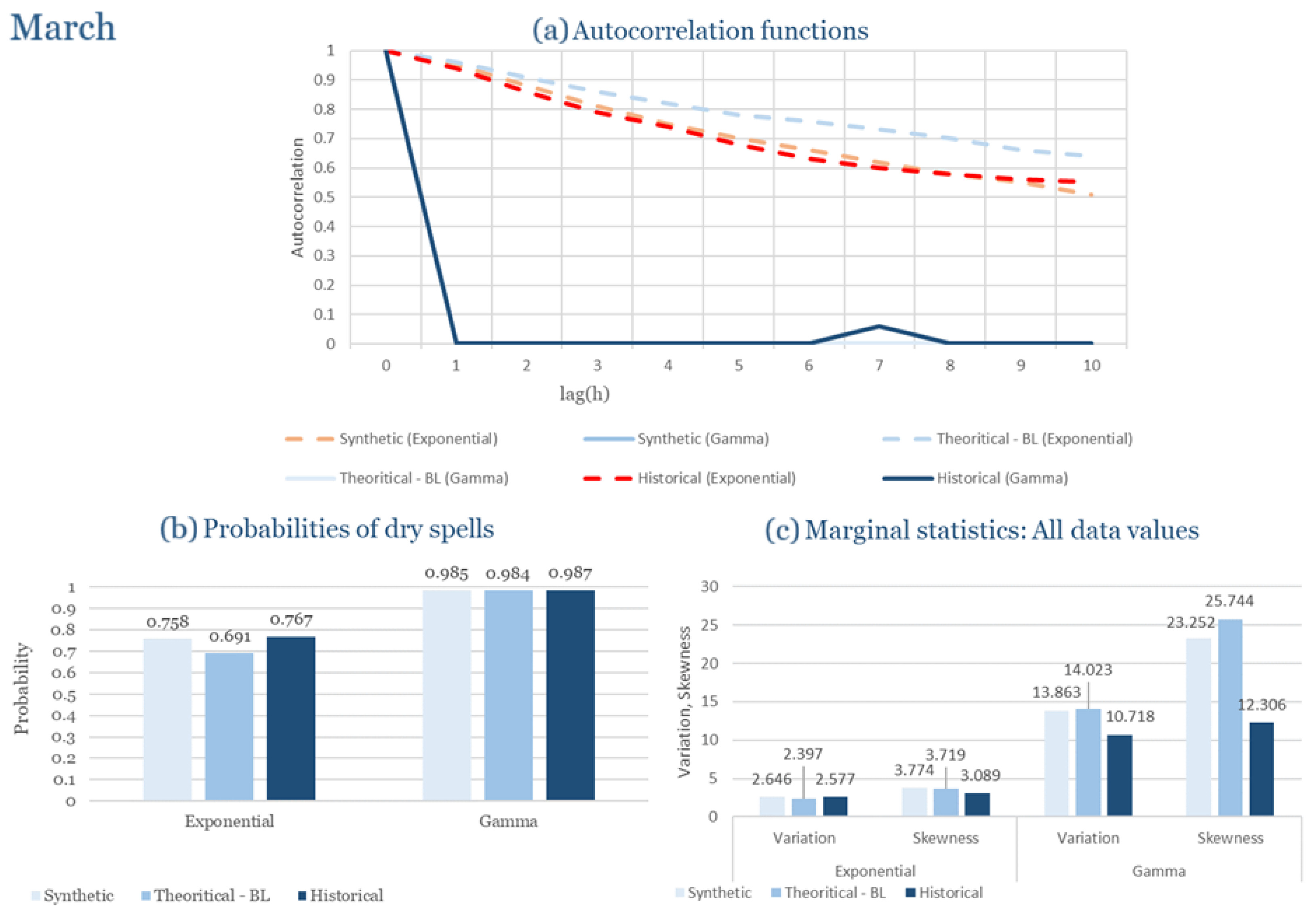
Statistical Characteristics of Corfu for March, with the intensity of the pulses following both distributions, where: (a) the diagram of the autocorrelation coefficient, (b) the diagram of the probability of dry and (c) the diagrams for the coefficient of variation and skewness of the historical and synthetic timeseries.
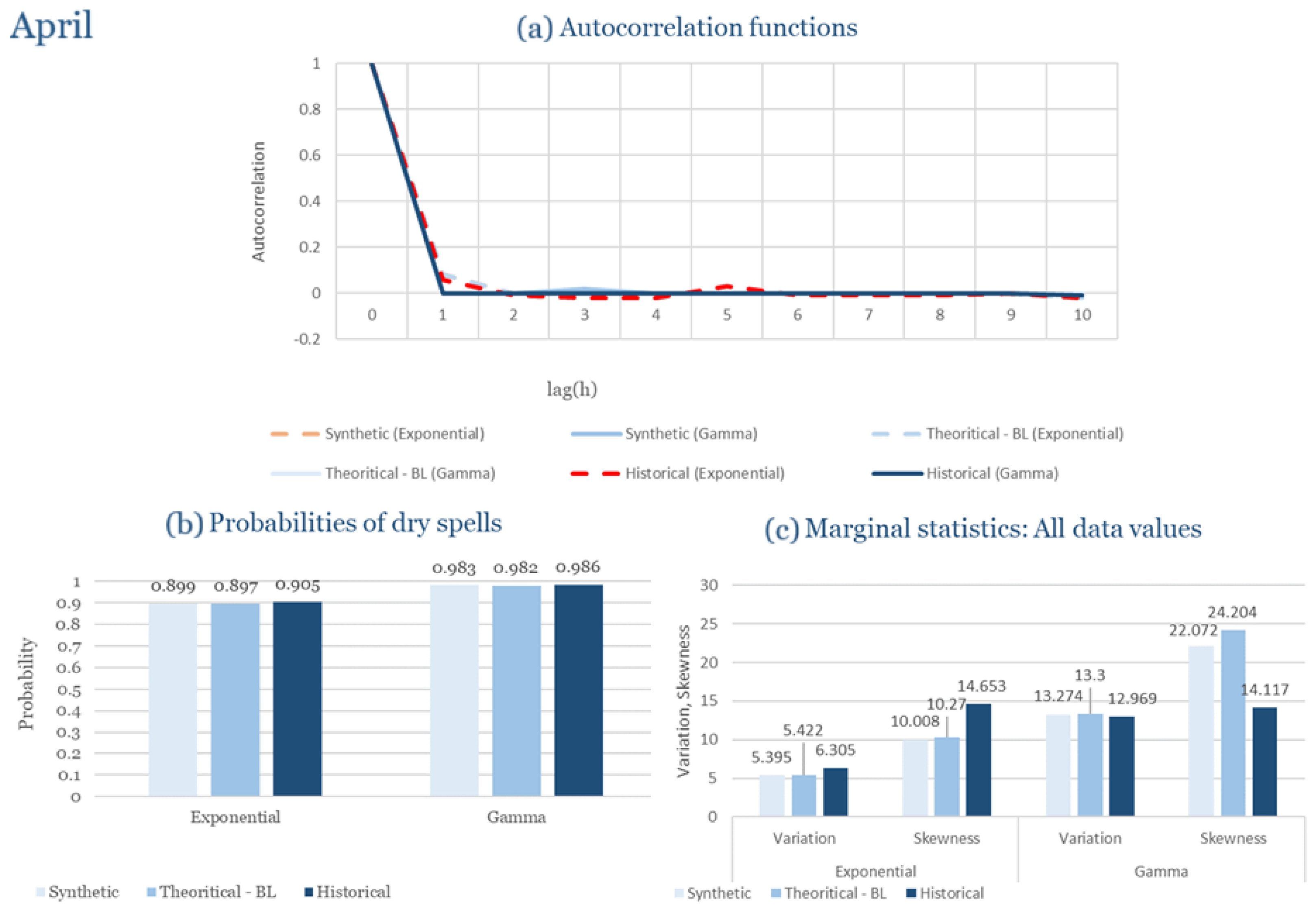
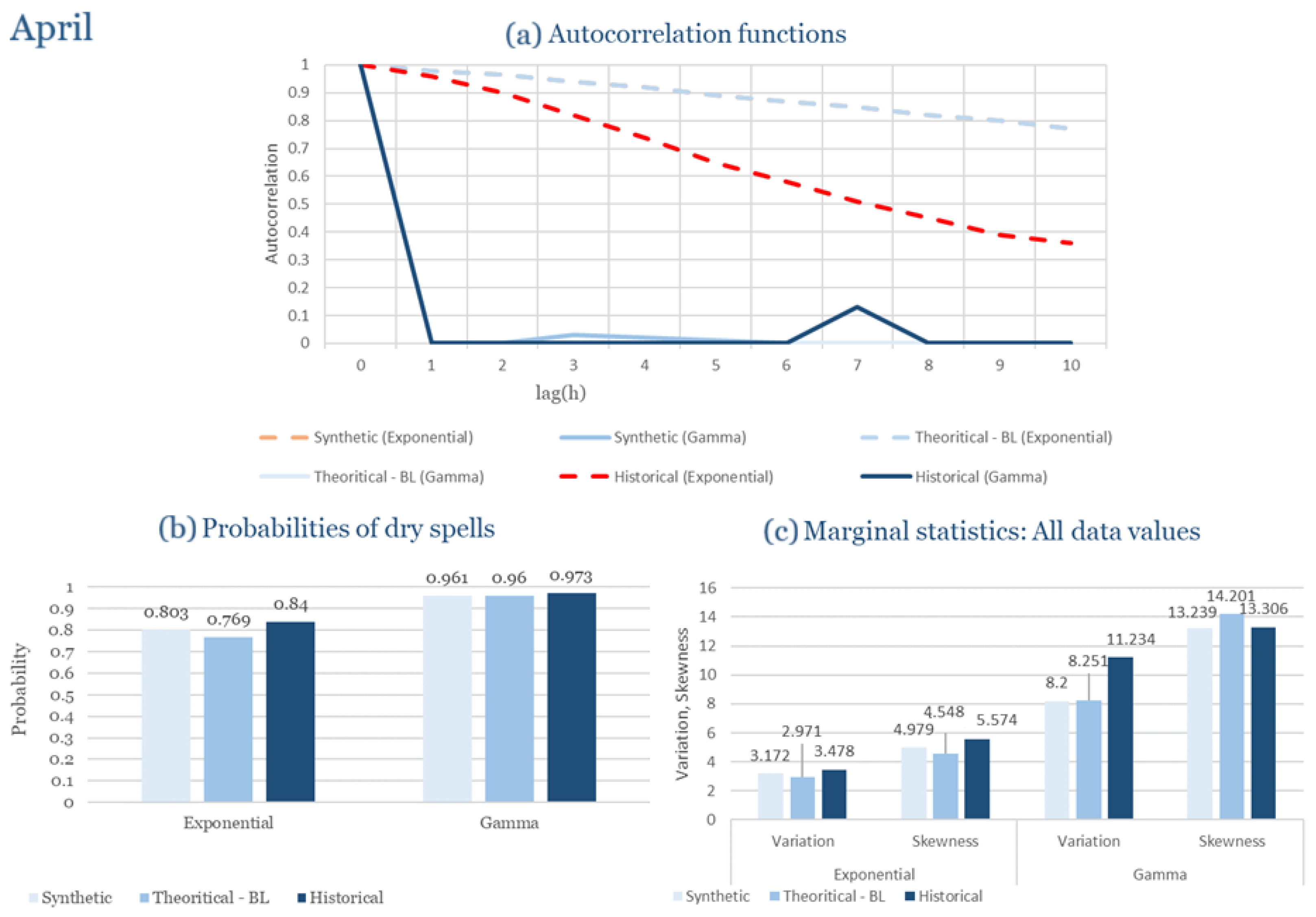
Figure A4.
Statistical Characteristics of Corfu for April, with the intensity of the pulses following both distributions, where: (a) the diagram of the autocorrelation coefficient, (b) the diagram of the probability of dry and (c) the diagrams for the coefficient of variation and skewness of the historical and synthetic timeseries.
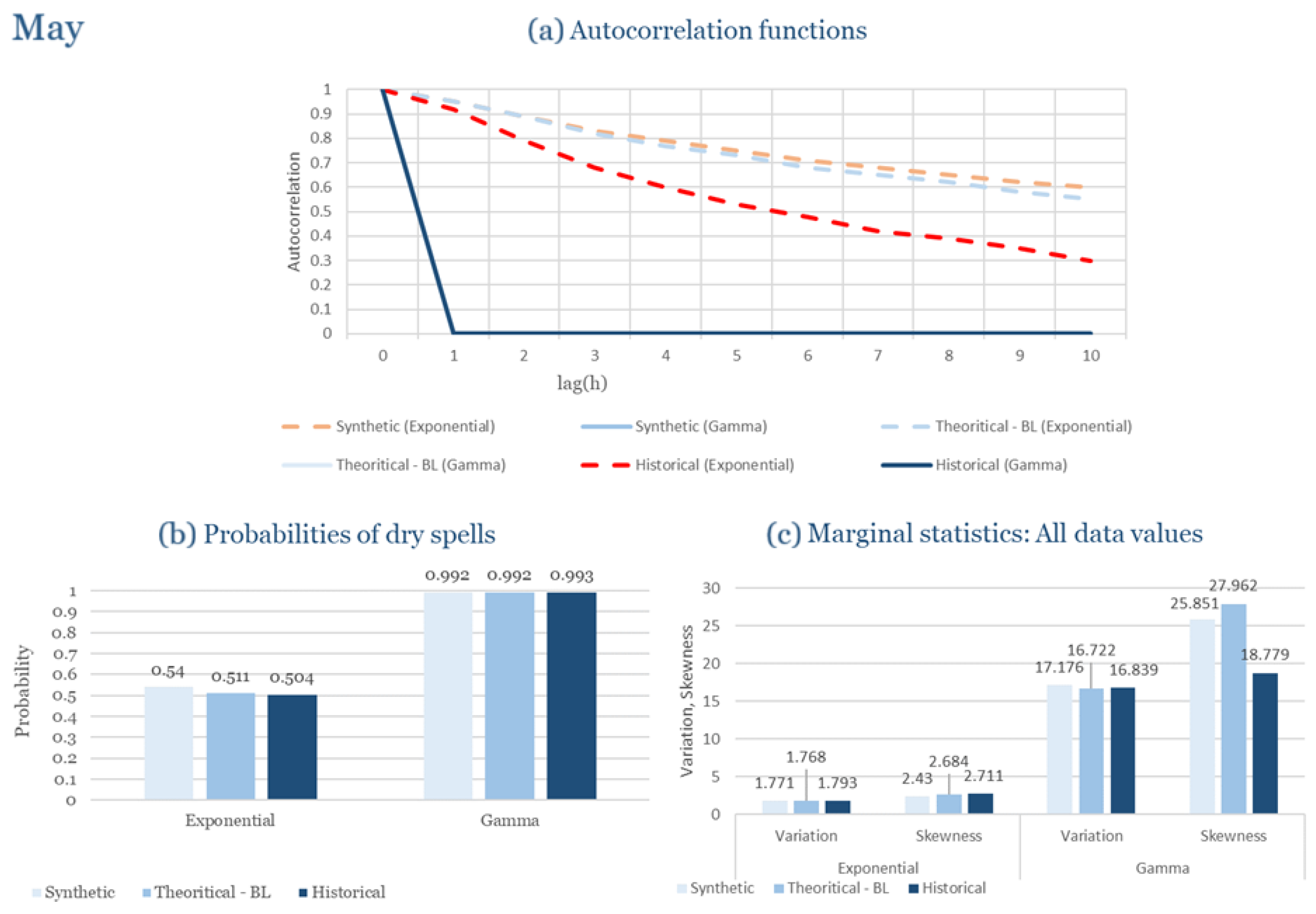
Figure A5.
Statistical Characteristics of Corfu for May, with the intensity of the pulses following both distributions, where: (a) the diagram of the autocorrelation coefficient, (b) the diagram of the probability of dry and (c) the diagrams for the coefficient of variation and skewness of the historical and synthetic timeseries.
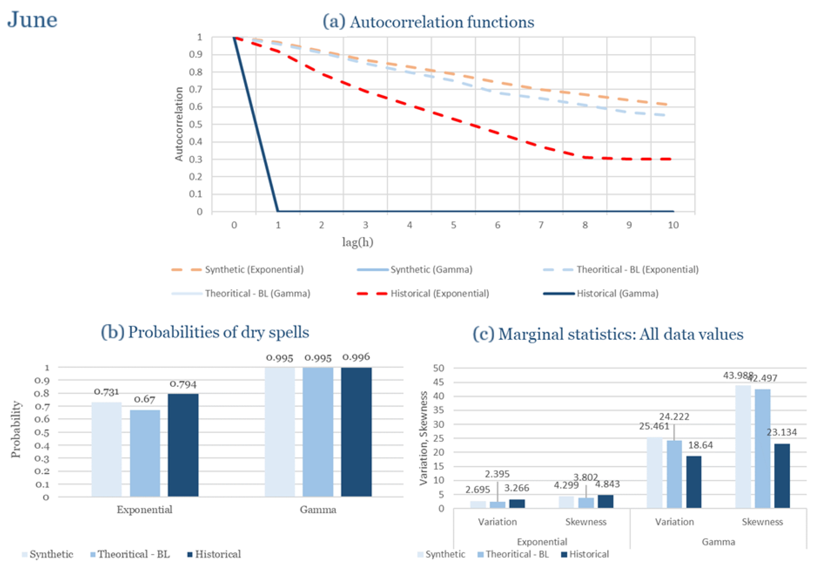
Figure A6.
Statistical Characteristics of Corfu for June, with the intensity of the pulses following both distributions, where: (a) the diagram of the autocorrelation coefficient, (b) the diagram of the probability of dry and (c) the diagrams for the coefficient of variation and skewness of the historical and synthetic timeseries.
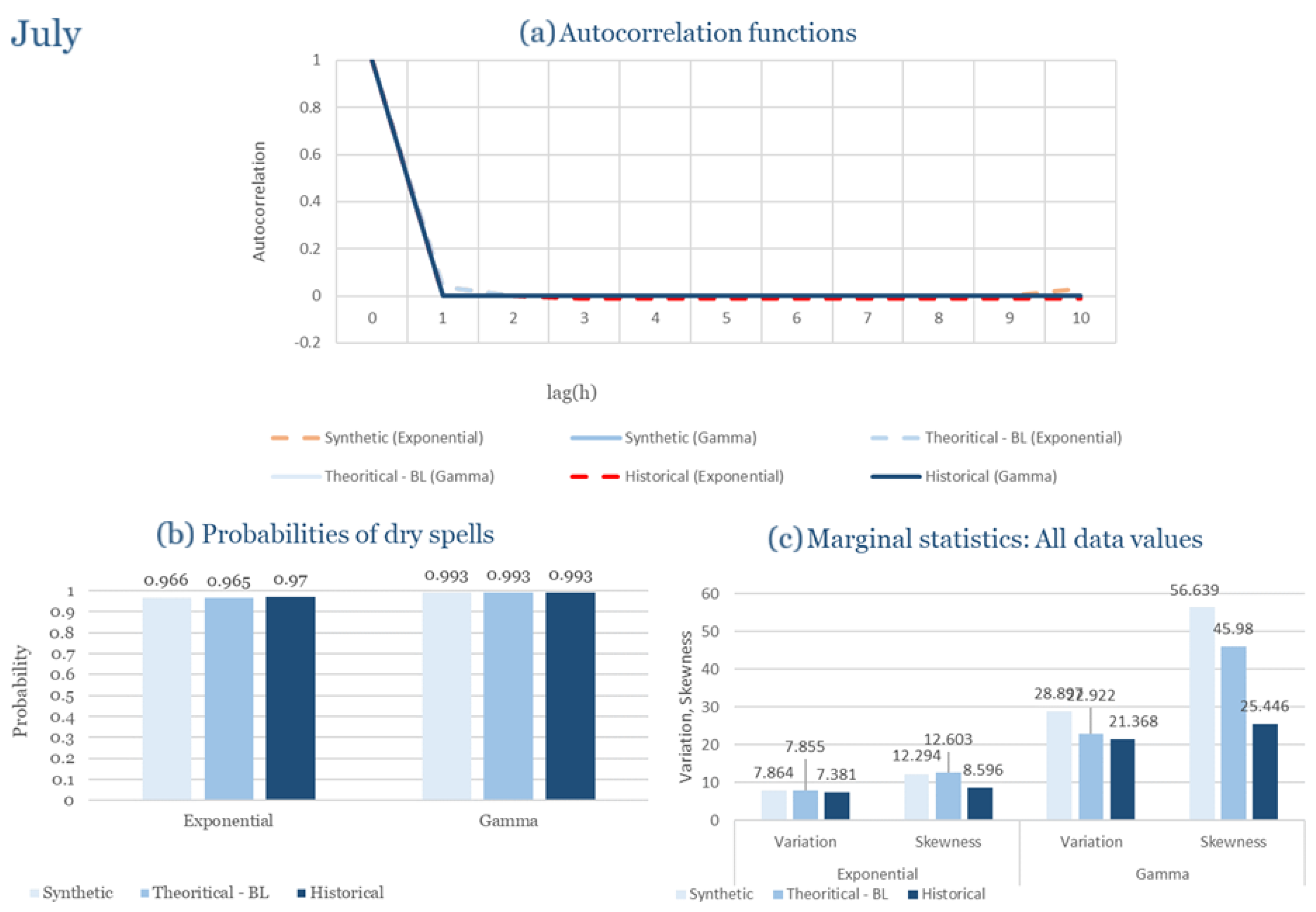
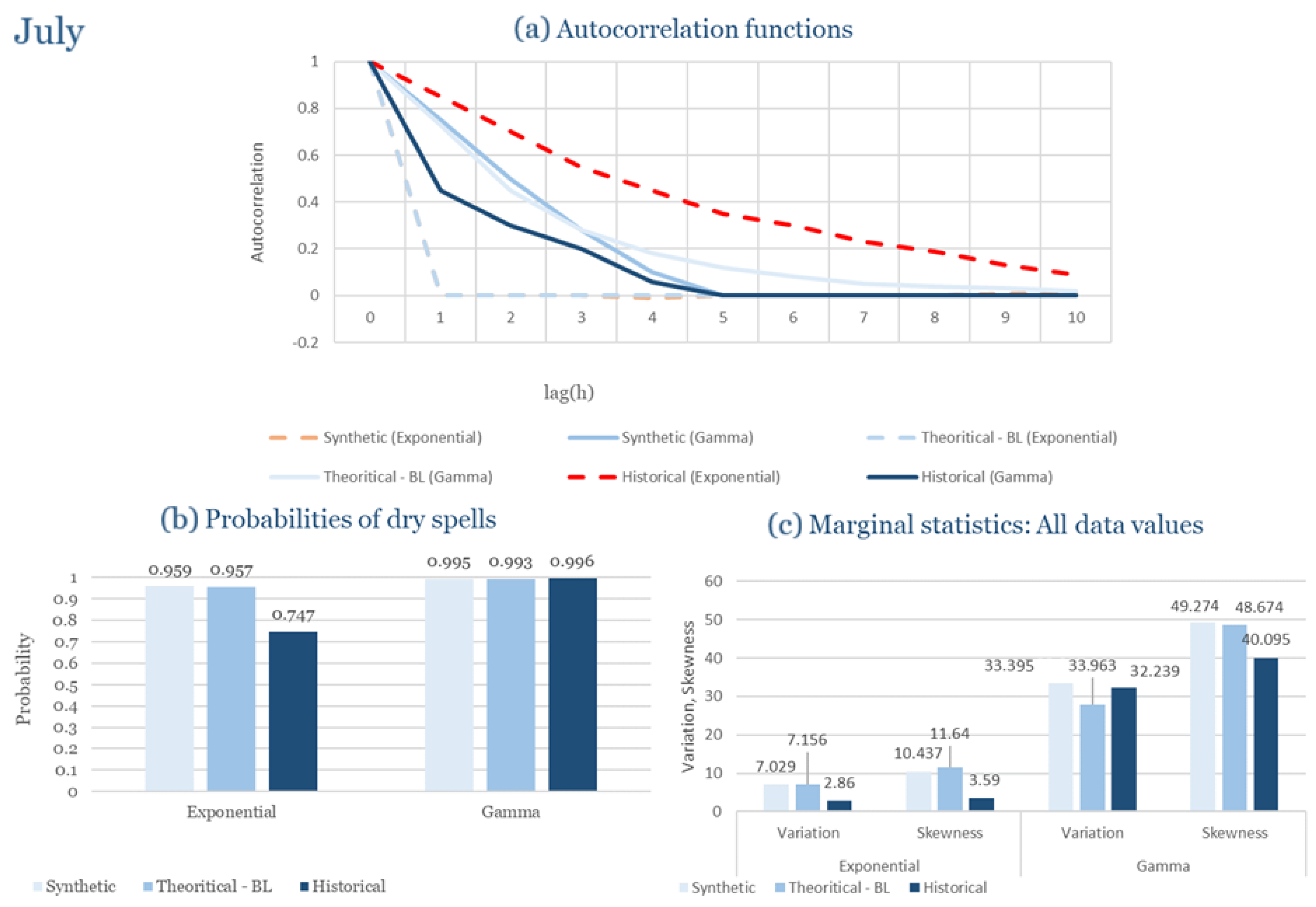
Figure A7.
Statistical Characteristics of Corfu for July, with the intensity of the pulses following both distributions, where: (a) the diagram of the autocorrelation coefficient, (b) the diagram of the probability of dry and (c) the diagrams for the coefficient of variation and skewness of the historical and synthetic timeseries.
Figure A8.
Statistical Characteristics of Corfu for August, with the intensity of the pulses following both distributions, where: (a) the diagram of the autocorrelation coefficient, (b) the diagram of the probability of dry and (c) the diagrams for the coefficient of variation and skewness of the historical and synthetic timeseries.
Figure A9.
Statistical Characteristics of Corfu for September, with the intensity of the pulses following both distributions, where: (a) the diagram of the autocorrelation coefficient, (b) the diagram of the probability of dry and (c) the diagrams for the coefficient of variation and skewness of the historical and synthetic timeseries.
Figure A10.
Statistical Characteristics of Corfu for October, with the intensity of the pulses following both distributions, where: (a) the diagram of the autocorrelation coefficient, (b) the diagram of the probability of dry and (c) the diagrams for the coefficient of variation and skewness of the historical and synthetic timeseries.
Figure A11.
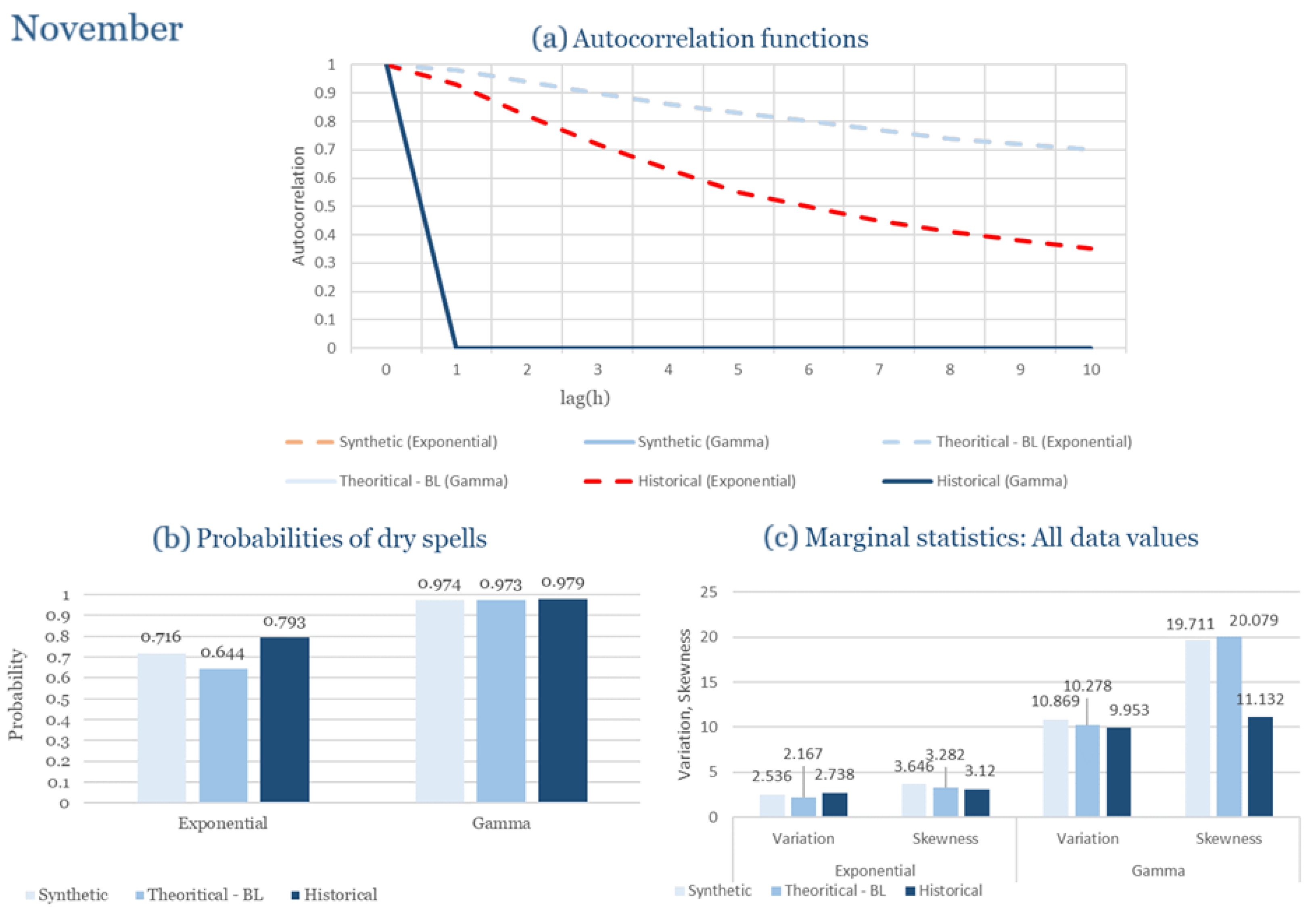
Statistical Characteristics of Corfu for November, with the intensity of the pulses following both distributions, where: (a) the diagram of the autocorrelation coefficient, (b) the diagram of the probability of dry and (c) the diagrams for the coefficient of variation and skewness of the historical and synthetic timeseries.
Figure A12.
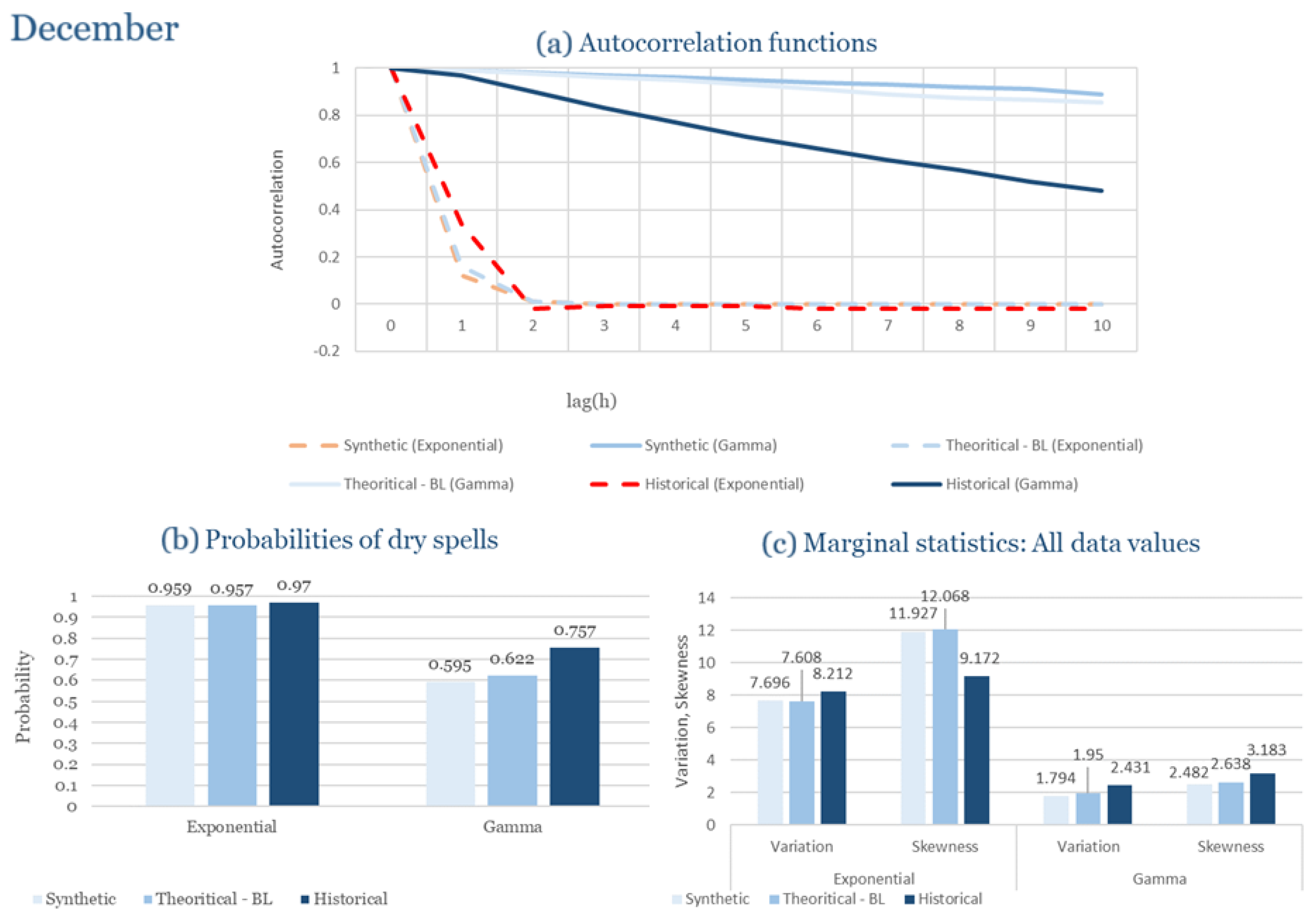
Statistical Characteristics of Corfu for December, with the intensity of the pulses following both distributions, where: (a) the diagram of the autocorrelation coefficient, (b) the diagram of the probability of dry and (c) the diagrams for the coefficient of variation and skewness of the historical and synthetic timeseries.
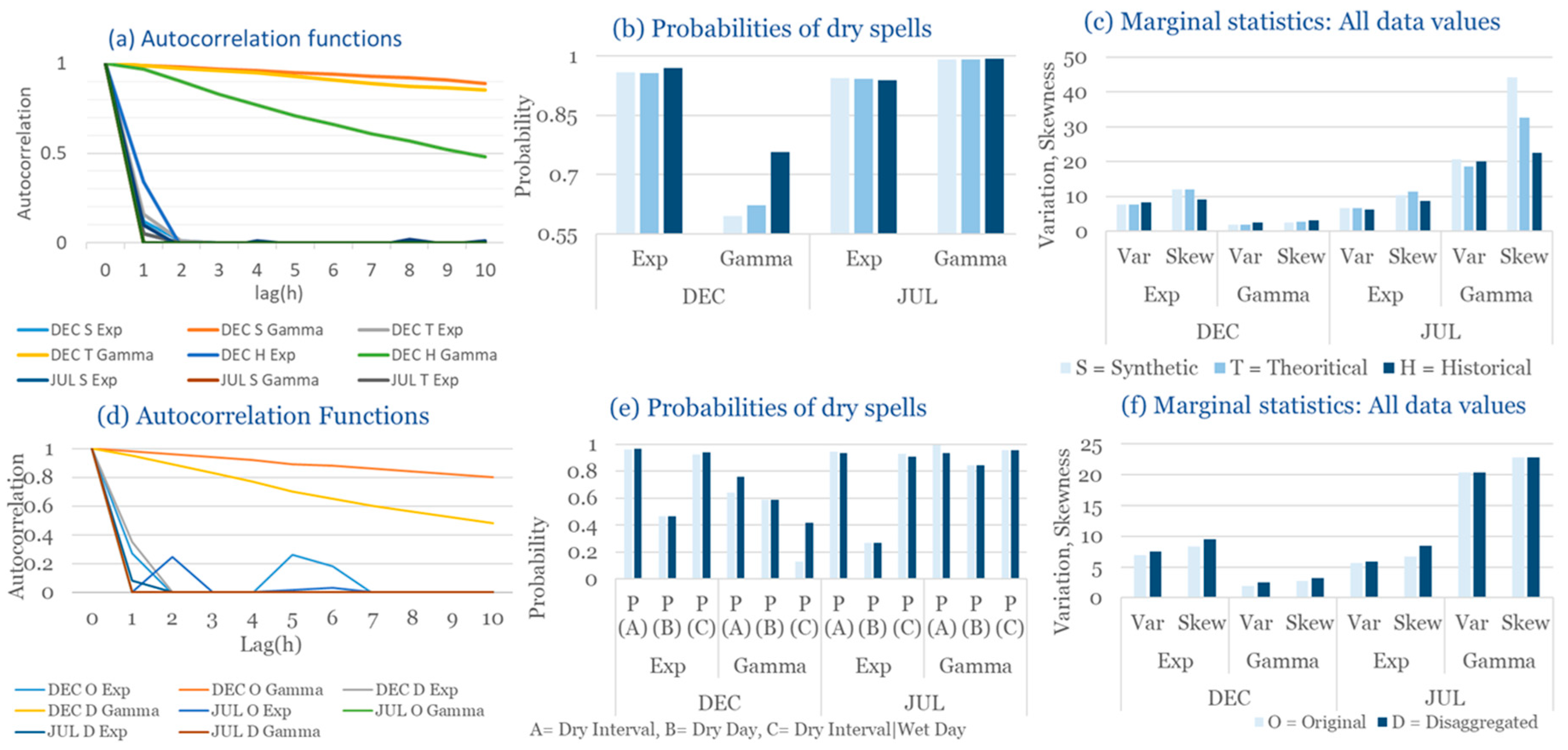
Figure A13.
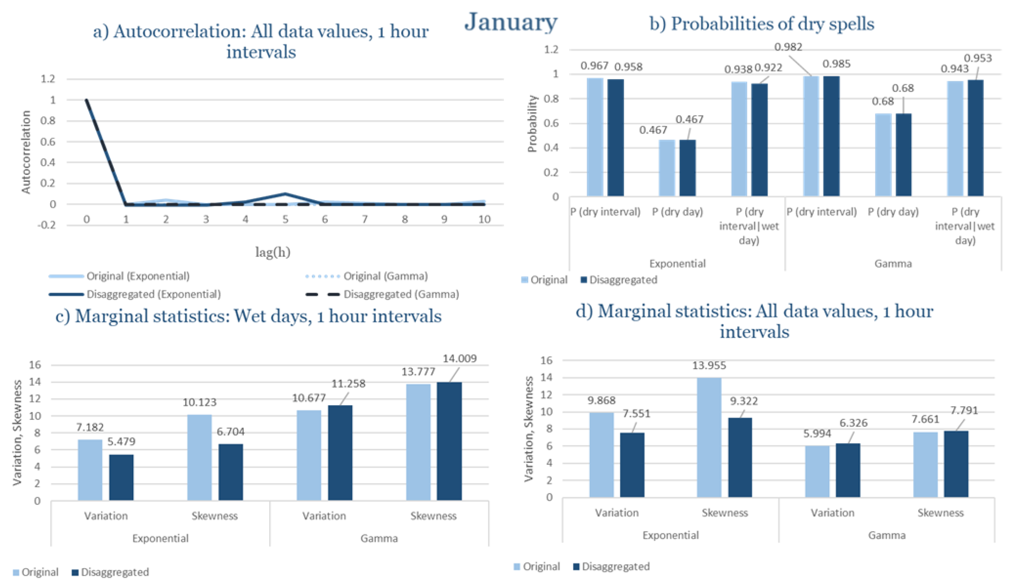
Statistical Characteristics of Corfu for January, with the intensity of the pulses following both distributions, where: (a) the diagram of the autocorrelation coefficient, (b) the diagrams of the probability of dry during a dry hour, a dry day and a dry hour||rainy day respectively, (c) the plots for the coefficient of variation and the coefficient of skewness of rainy days and (d) the plots for the coefficient of variation and the coefficient skewness for all data of the respective disagreggated time series.
Figure A14.
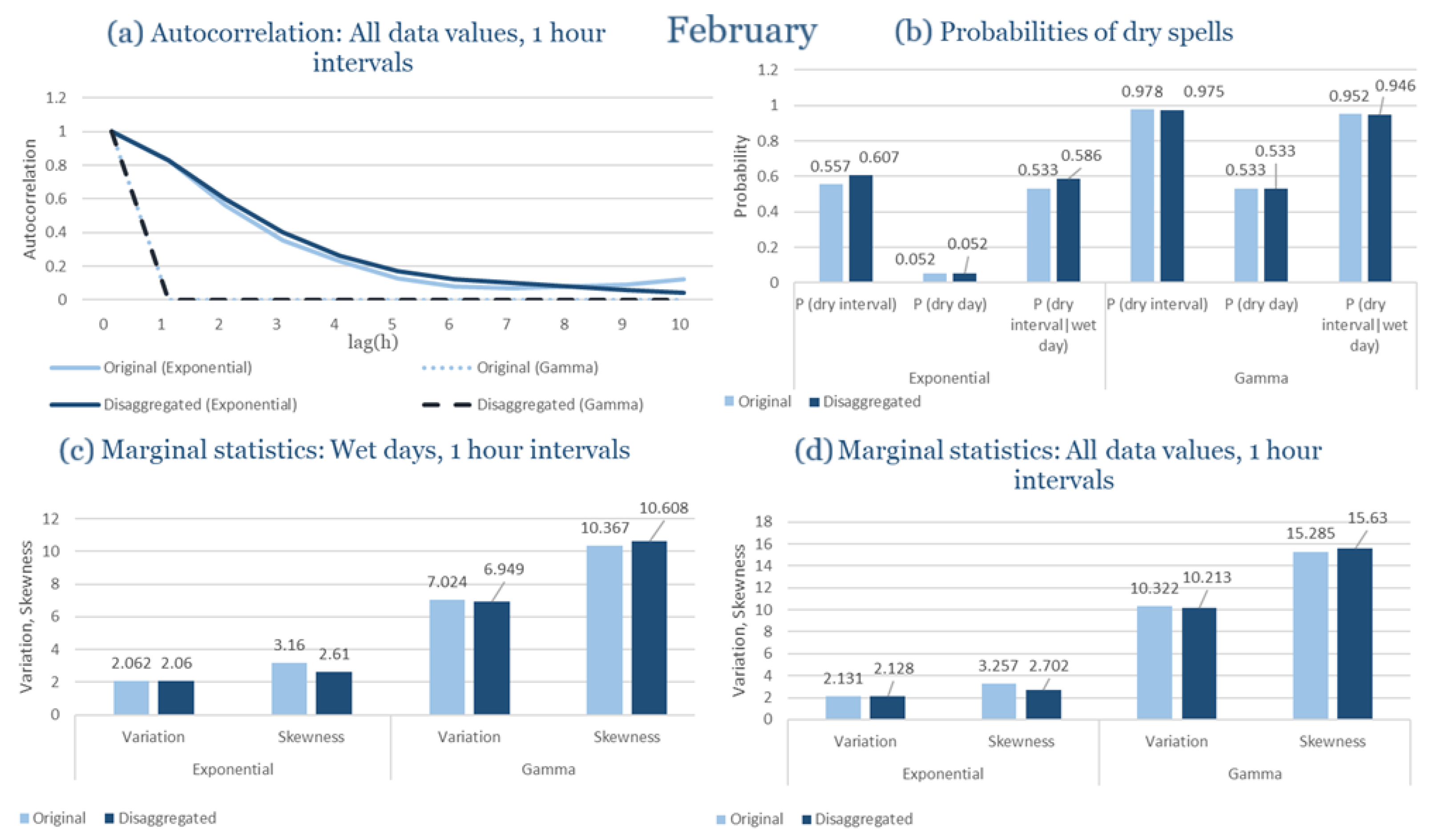
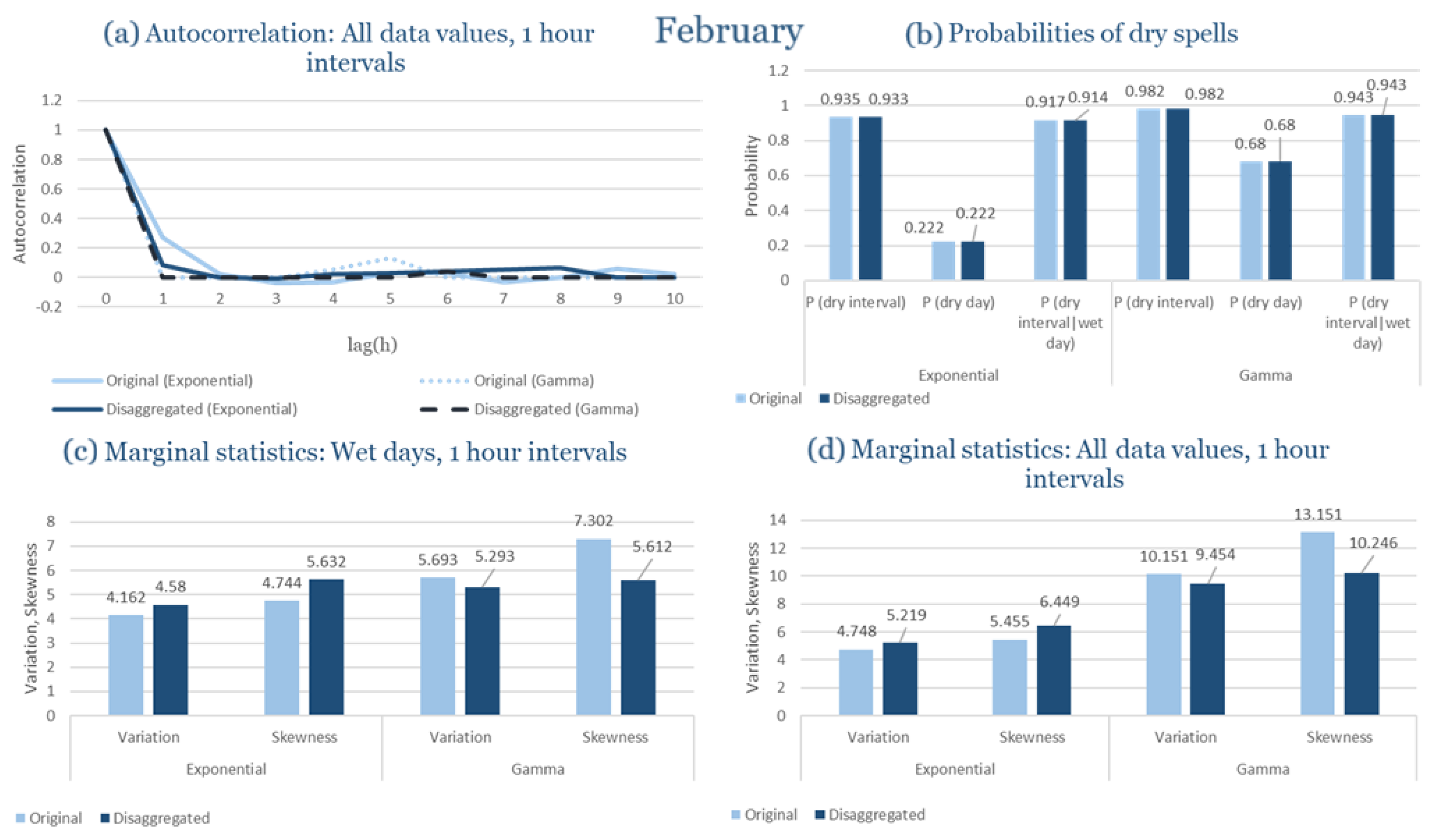
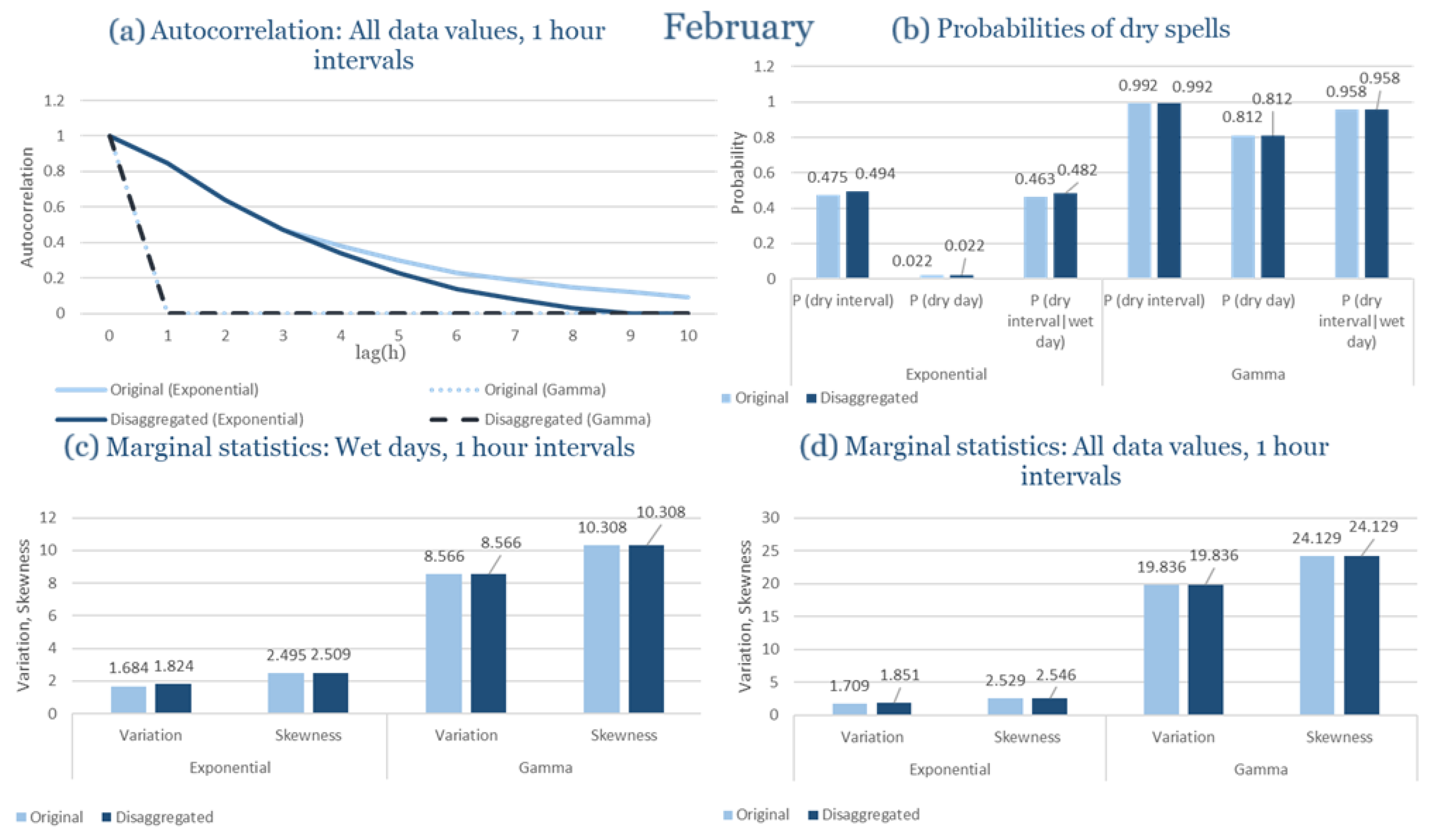
Statistical Characteristics of Corfu for February, with the intensity of the pulses following both distributions, where: (a) the diagram of the autocorrelation coefficient, (b) the diagrams of the probability of dry during a dry hour, a dry day and a dry hour||rainy day respectively, (c) the plots for the coefficient of variation and the coefficient of skewness of rainy days and (d) the plots for the coefficient of variation and the coefficient skewness for all data of the respective disagreggated time series.
Figure A15.
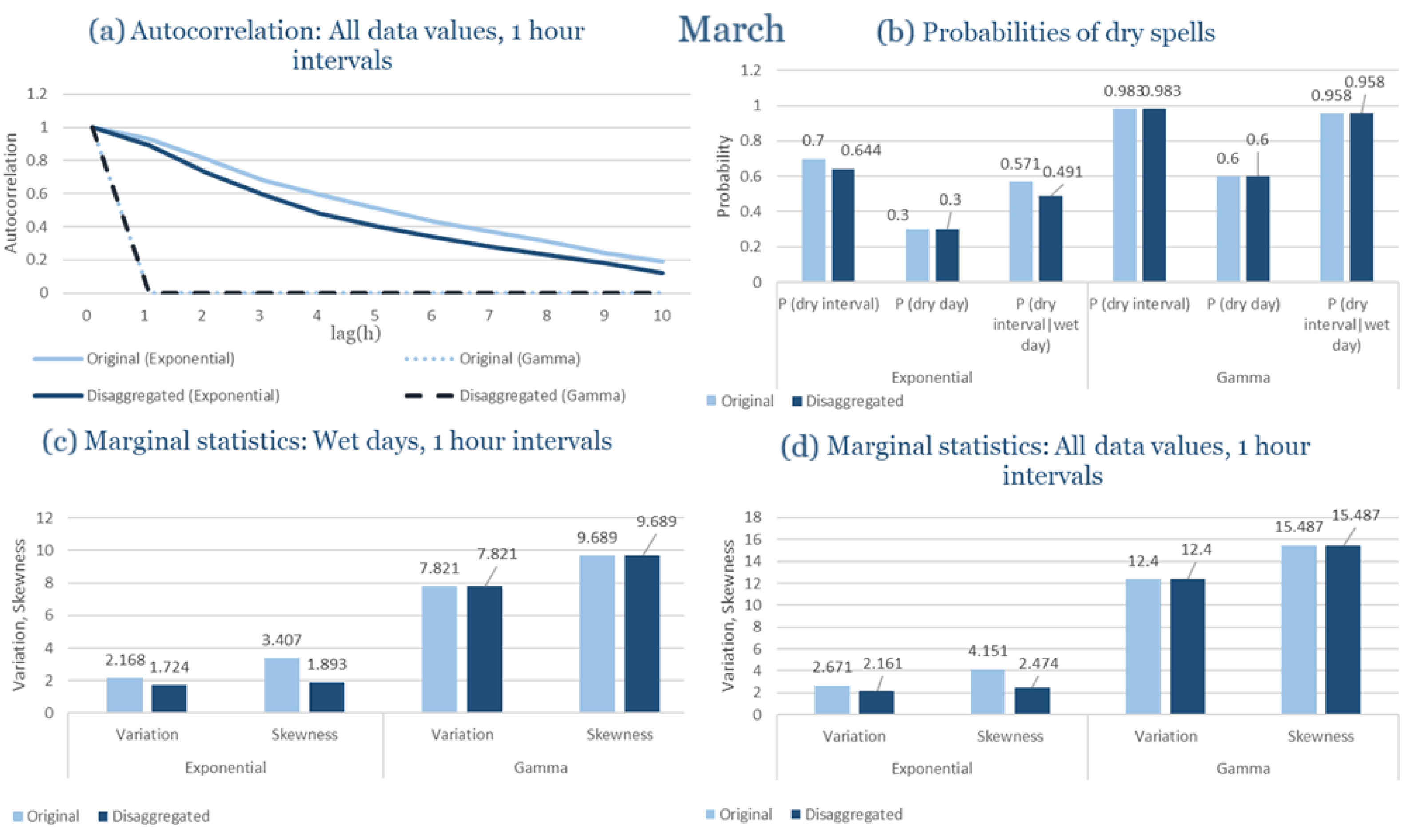
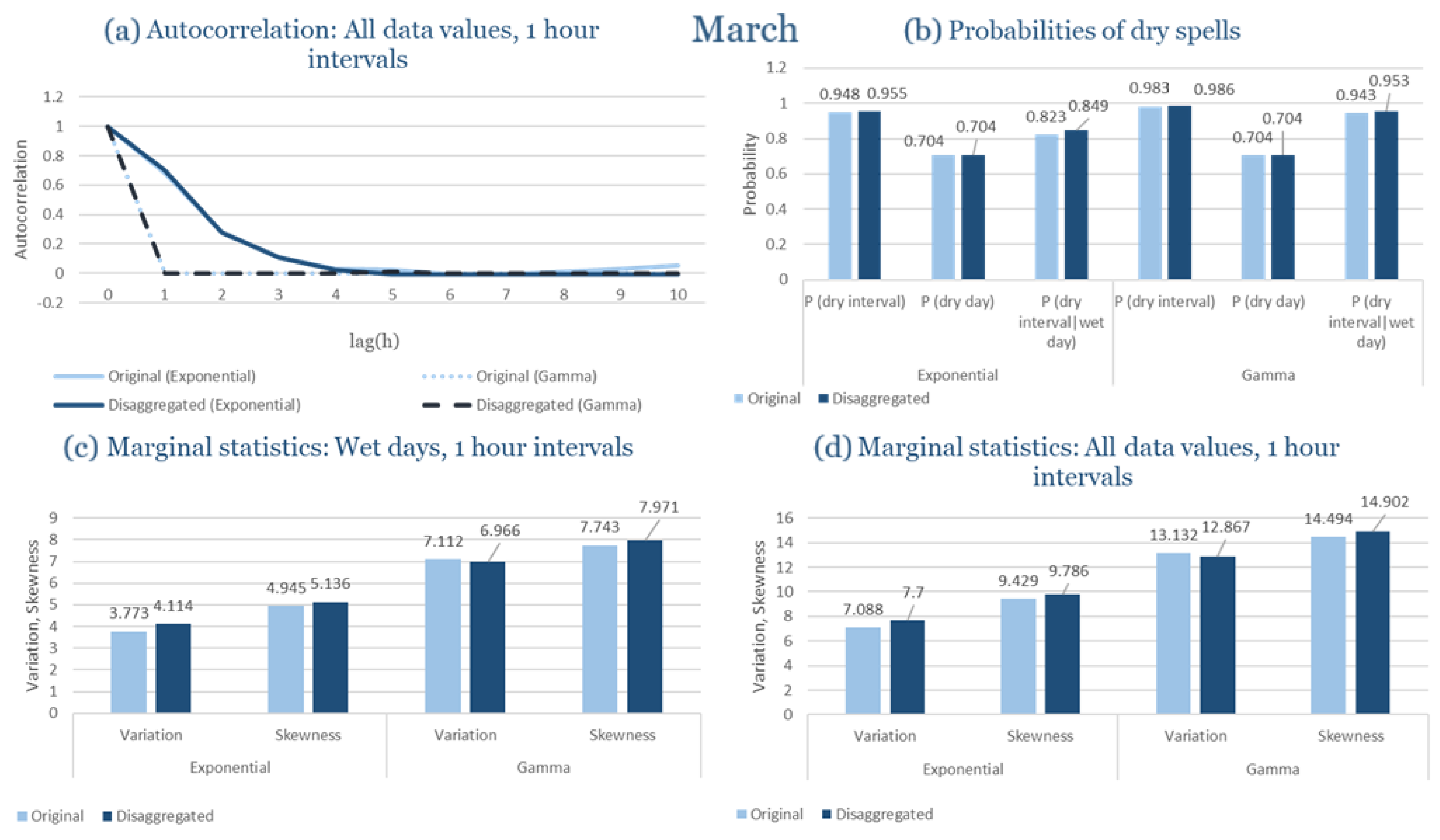
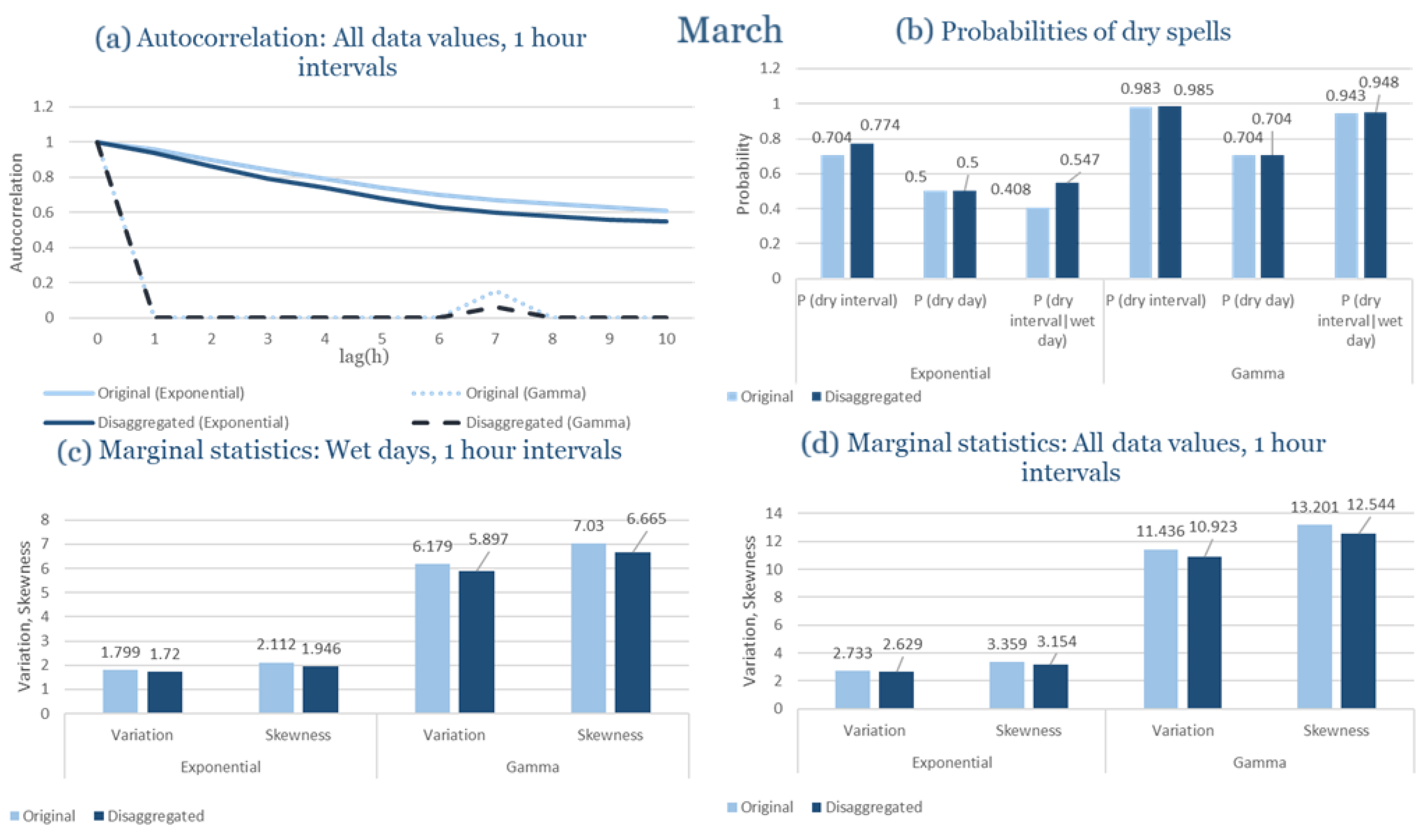
Statistical Characteristics of Corfu for March, with the intensity of the pulses following both distributions, where: (a) the diagram of the autocorrelation coefficient, (b) the diagrams of the probability of dry during a dry hour, a dry day and a dry hour||rainy day respectively, (c) the plots for the coefficient of variation and the coefficient of skewness of rainy days and (d) the plots for the coefficient of variation and the coefficient skewness for all data of the respective disagreggated time series.
Figure A16.
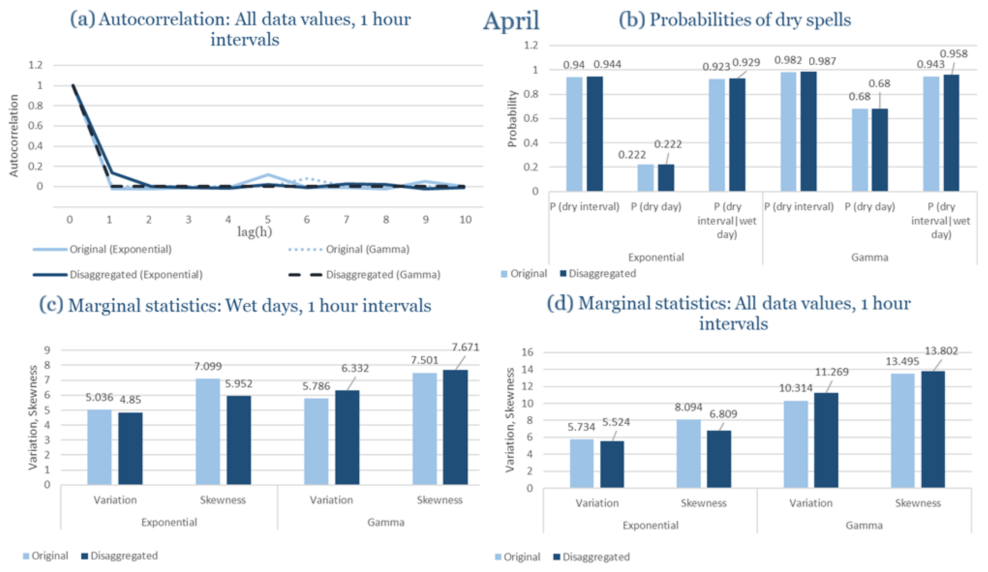
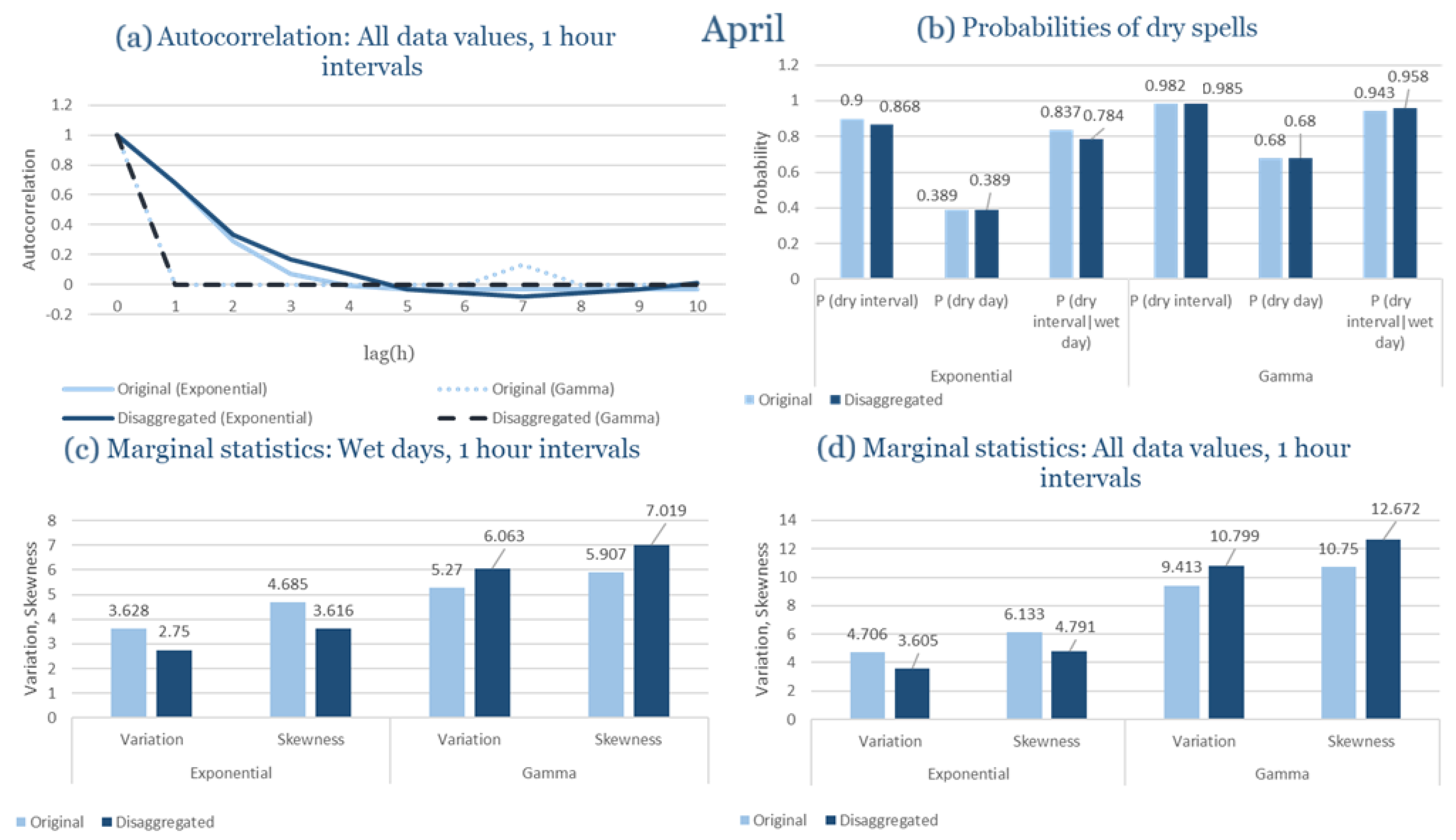
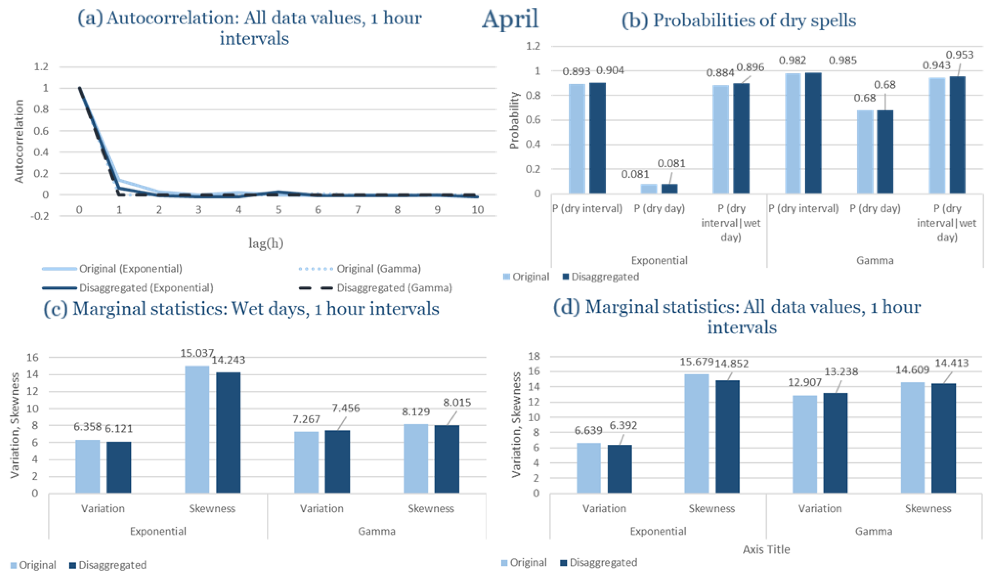
Statistical Characteristics of Corfu for April, with the intensity of the pulses following both distributions, where: (a) the diagram of the autocorrelation coefficient, (b) the diagrams of the probability of dry during a dry hour, a dry day and a dry hour||rainy day respectively, (c) the plots for the coefficient of variation and the coefficient of skewness of rainy days and (d) the plots for the coefficient of variation and the coefficient skewness for all data of the respective disagreggated time series.
Figure A17.
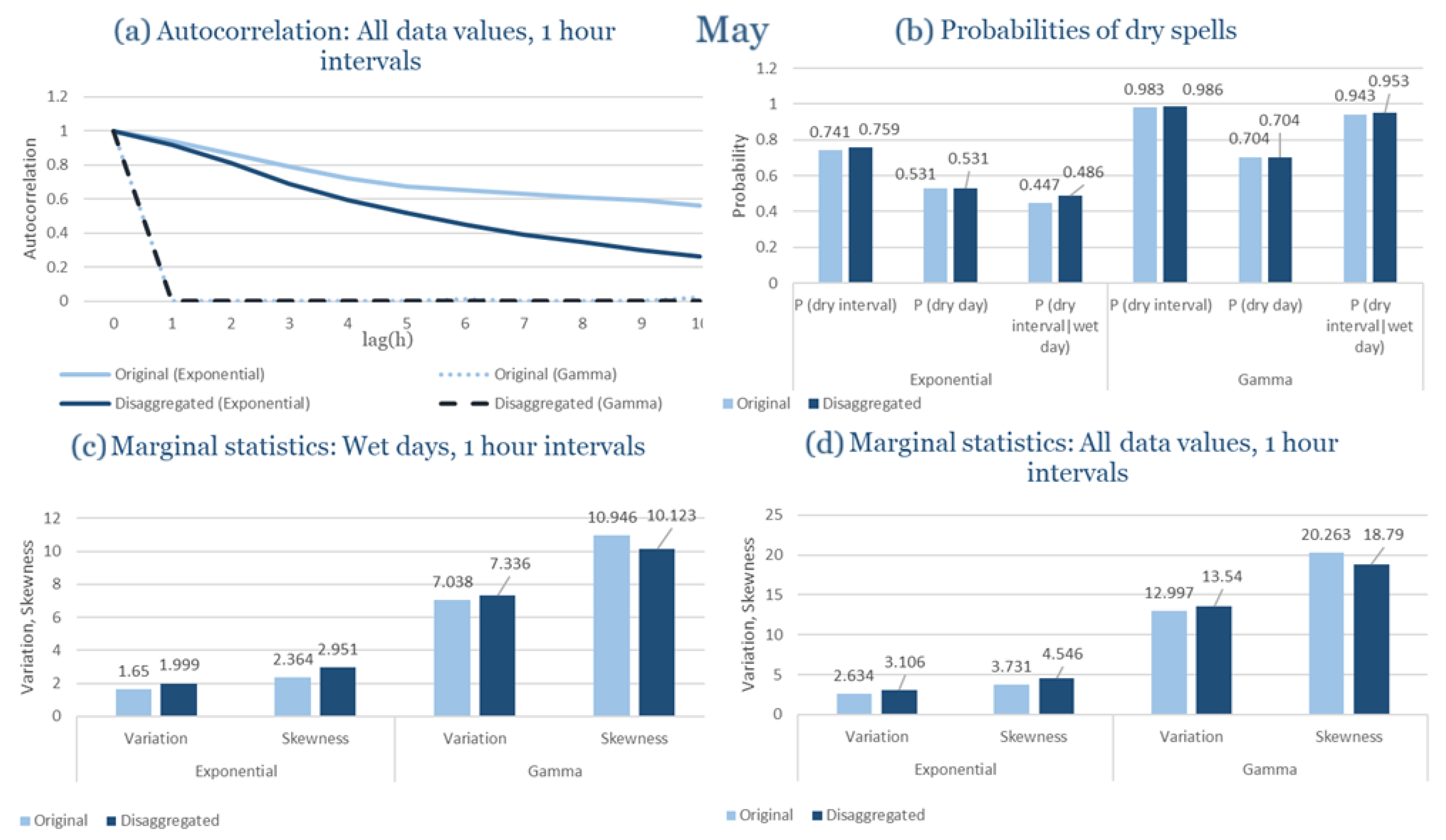
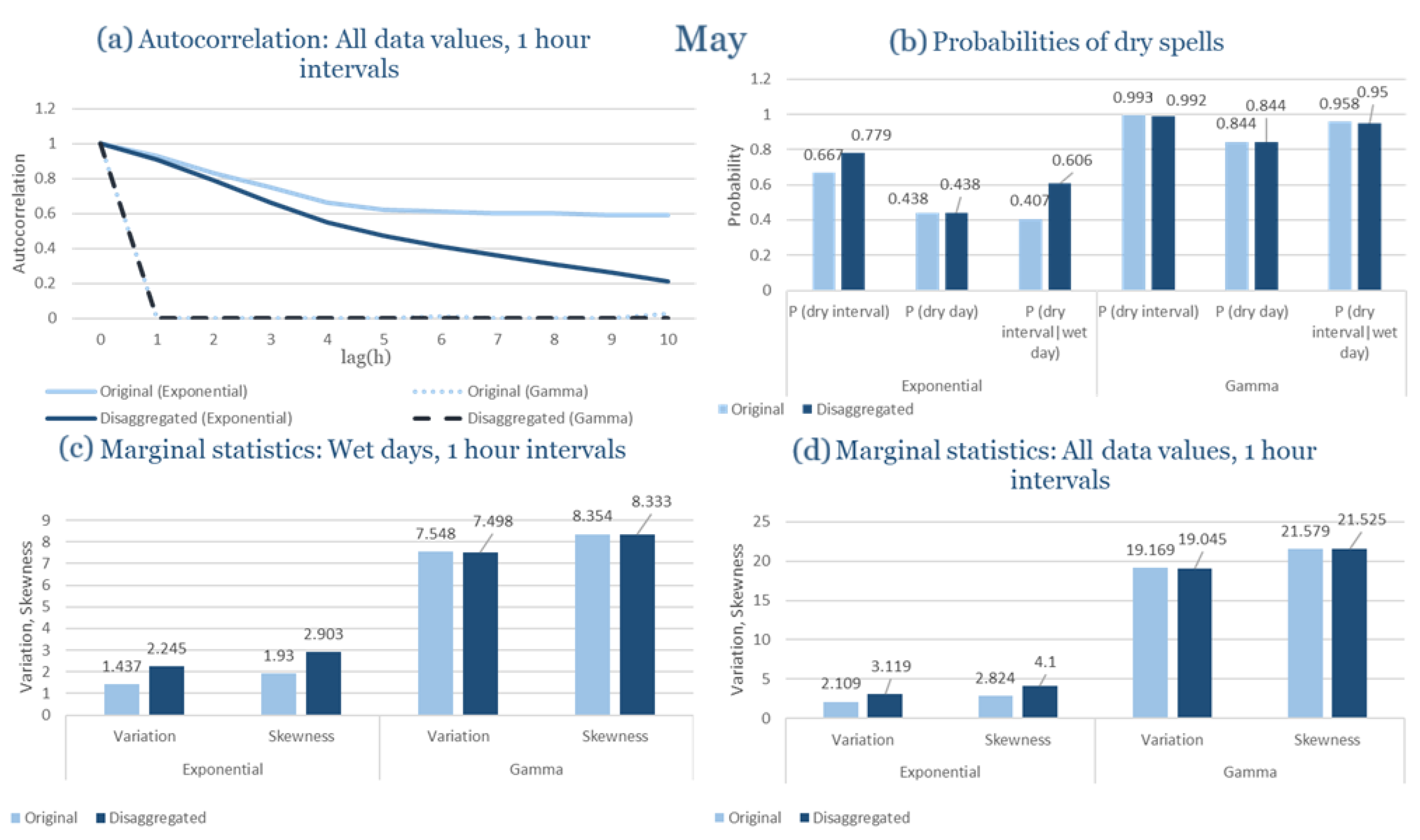
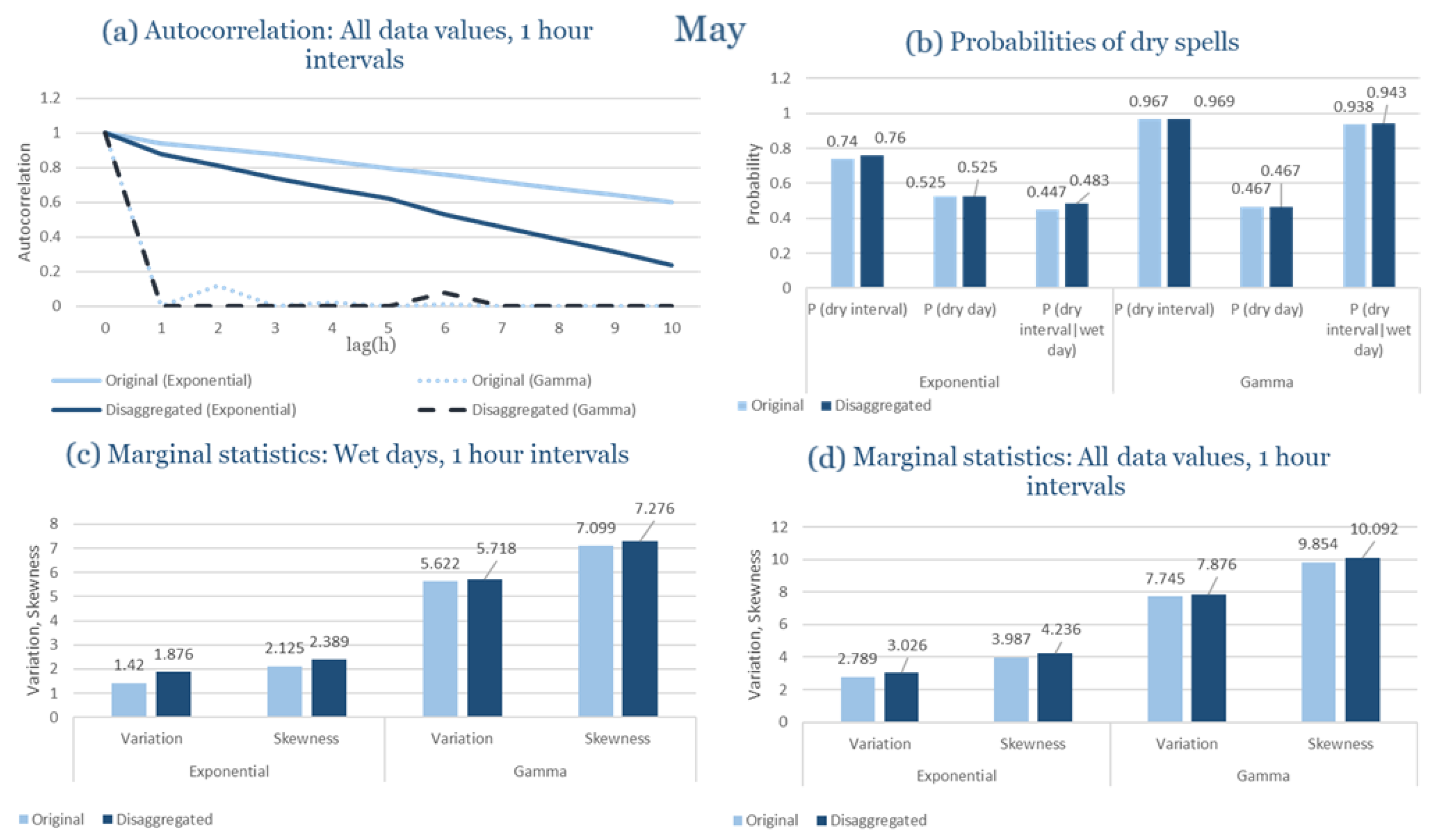
Statistical Characteristics of Corfu for May, with the intensity of the pulses following both distributions, where: (a) the diagram of the autocorrelation coefficient, (b) the diagrams of the probability of dry during a dry hour, a dry day and a dry hour||rainy day respectively, (c) the plots for the coefficient of variation and the coefficient of skewness of rainy days and (d) the plots for the coefficient of variation and the coefficient skewness for all data of the respective disagreggated time series.
Figure A18.
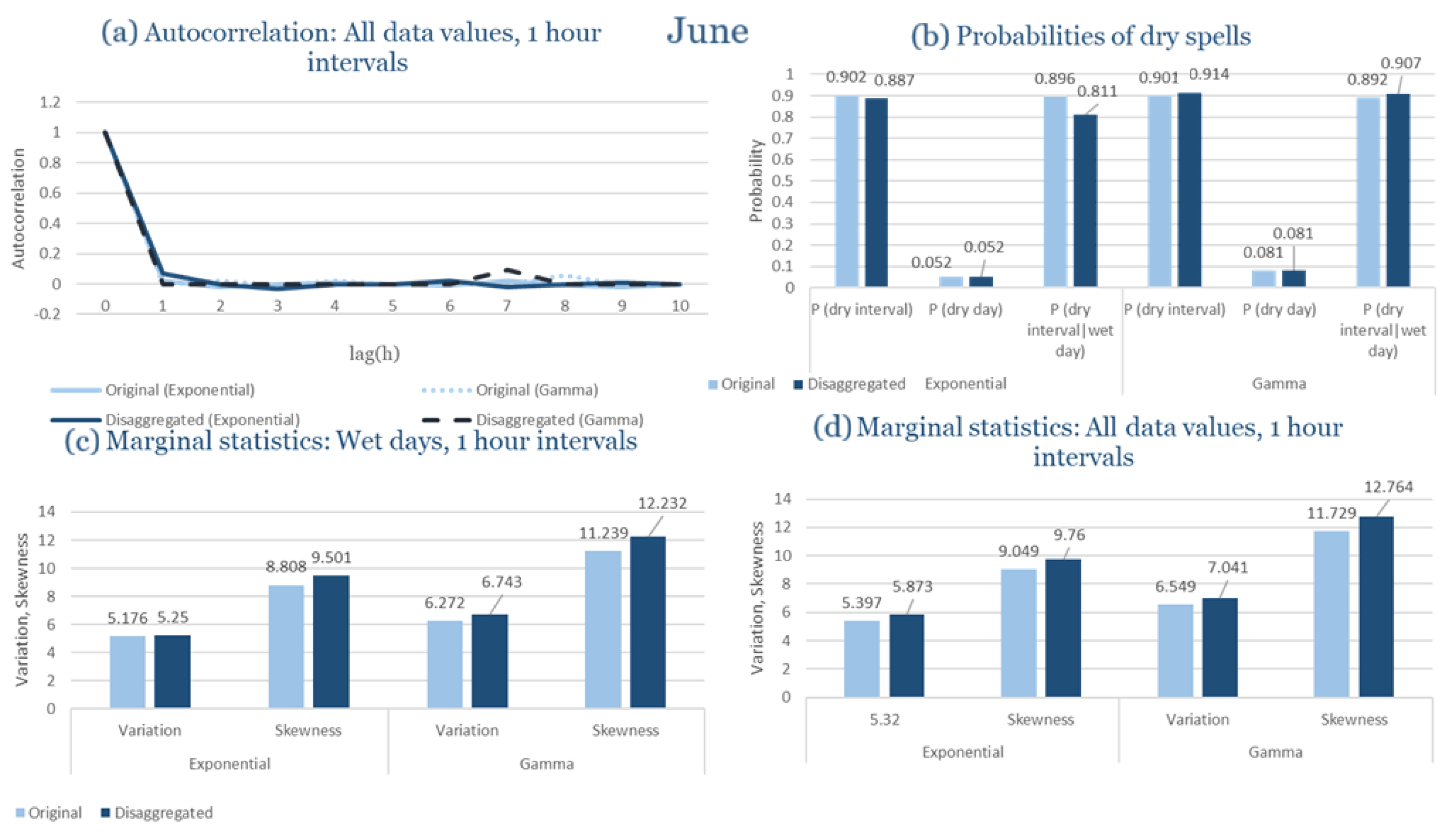
Statistical Characteristics of Corfu for June, with the intensity of the pulses following both distributions, where: (a) the diagram of the autocorrelation coefficient, (b) the diagrams of the probability of dry during a dry hour, a dry day and a dry hour||rainy day respectively, (c) the plots for the coefficient of variation and the coefficient of skewness of rainy days and (d) the plots for the coefficient of variation and the coefficient skewness for all data of the respective disagreggated time series.
Figure A19.
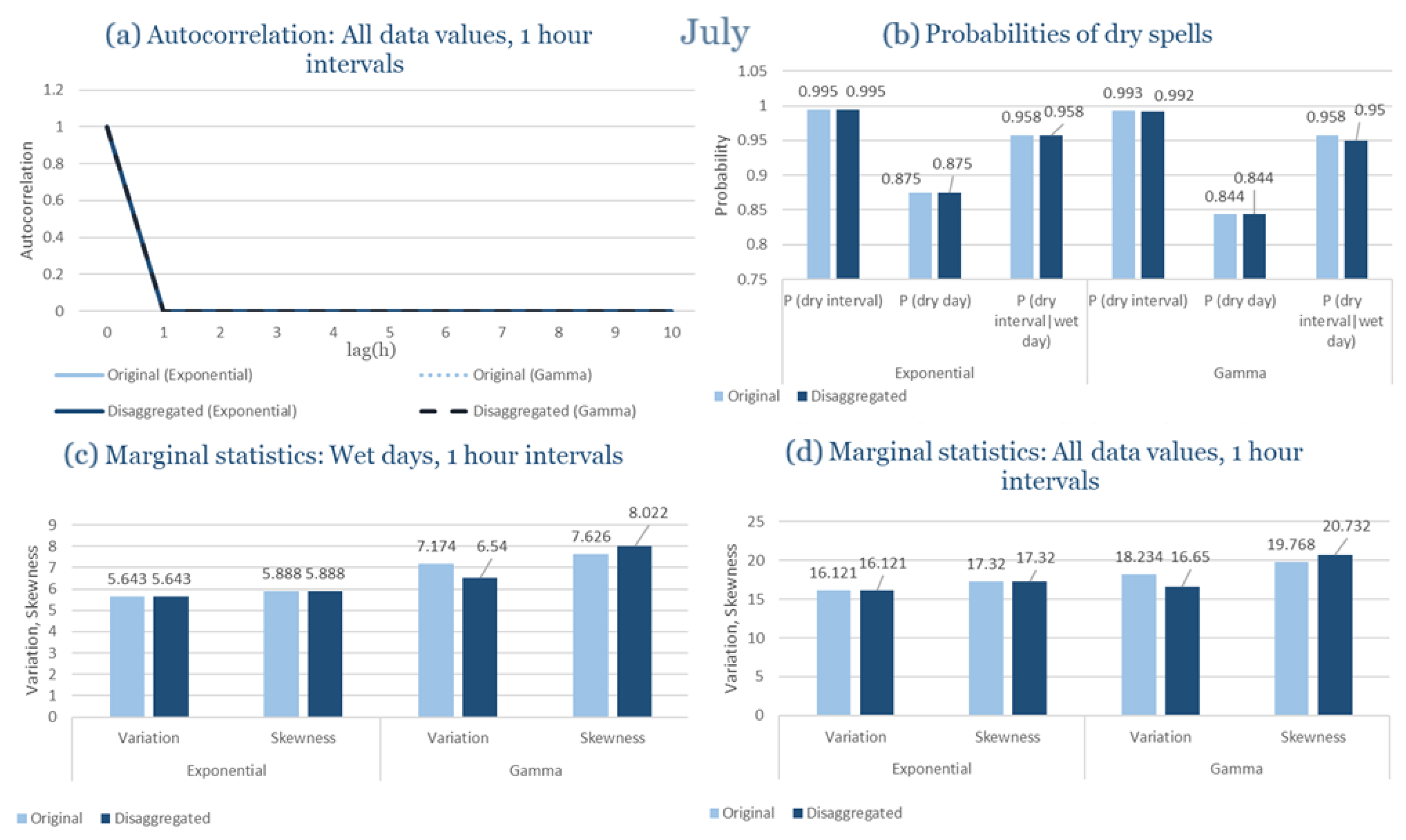
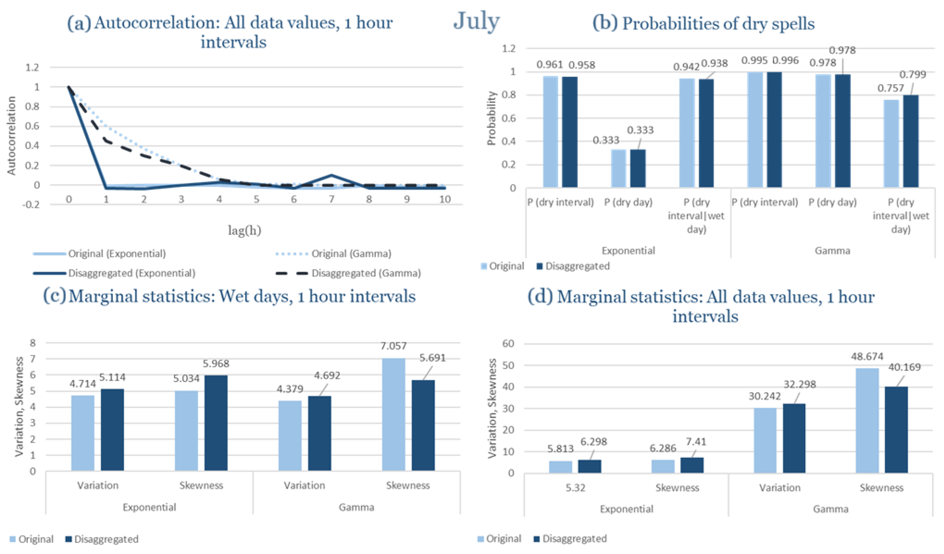
Statistical Characteristics of Corfu for July, with the intensity of the pulses following both distributions, where: (a) the diagram of the autocorrelation coefficient, (b) the diagrams of the probability of dry during a dry hour, a dry day and a dry hour||rainy day respectively, (c) the plots for the coefficient of variation and the coefficient of skewness of rainy days and (d) the plots for the coefficient of variation and the coefficient skewness for all data of the respective disagreggated time series.
Figure A20.
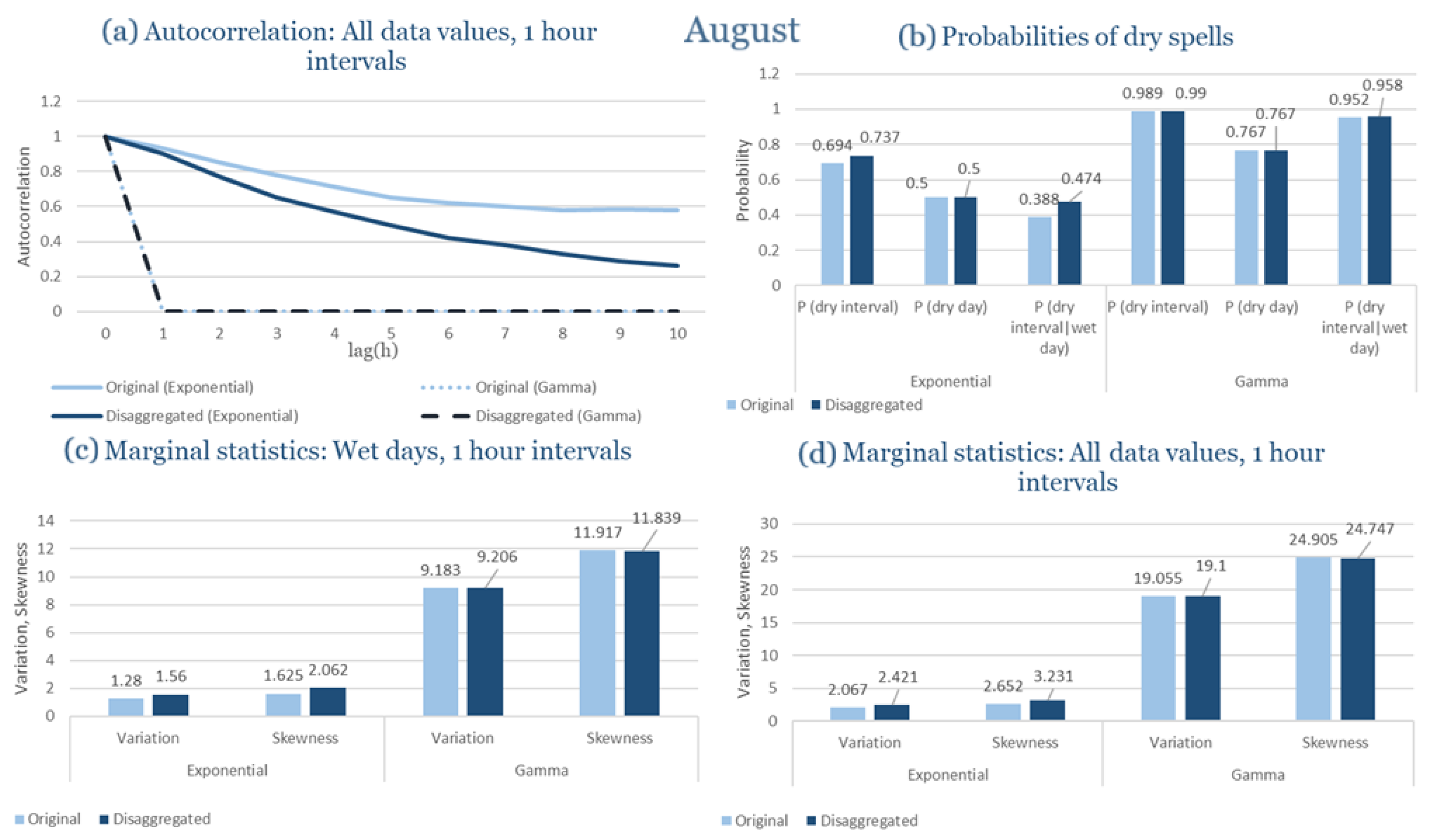
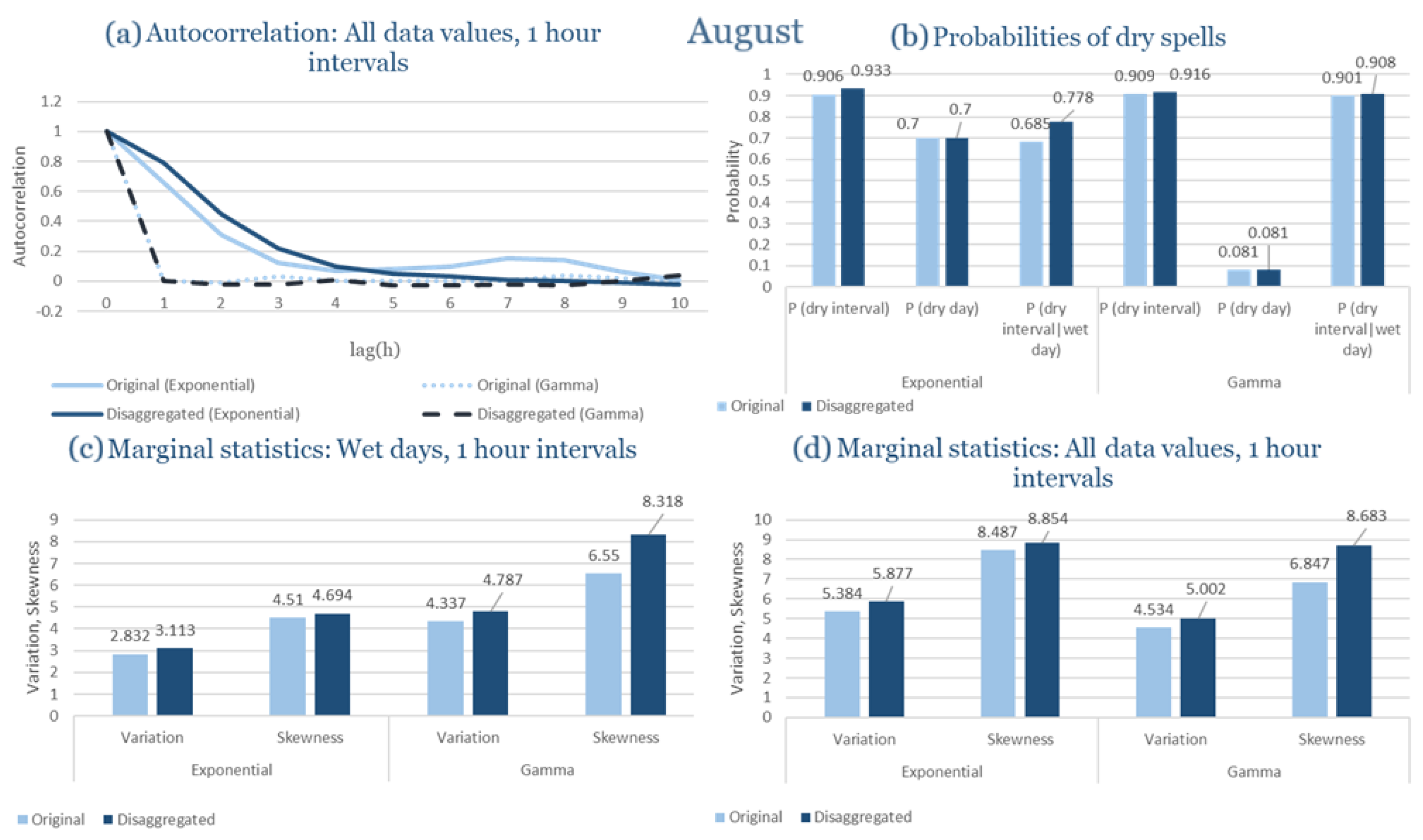
Statistical Characteristics of Corfu for August, with the intensity of the pulses following both distributions, where: (a) the diagram of the autocorrelation coefficient, (b) the diagrams of the probability of dry during a dry hour, a dry day and a dry hour||rainy day respectively, (c) the plots for the coefficient of variation and the coefficient of skewness of rainy days and (d) the plots for the coefficient of variation and the coefficient skewness for all data of the respective disagreggated time series.
Figure A21.
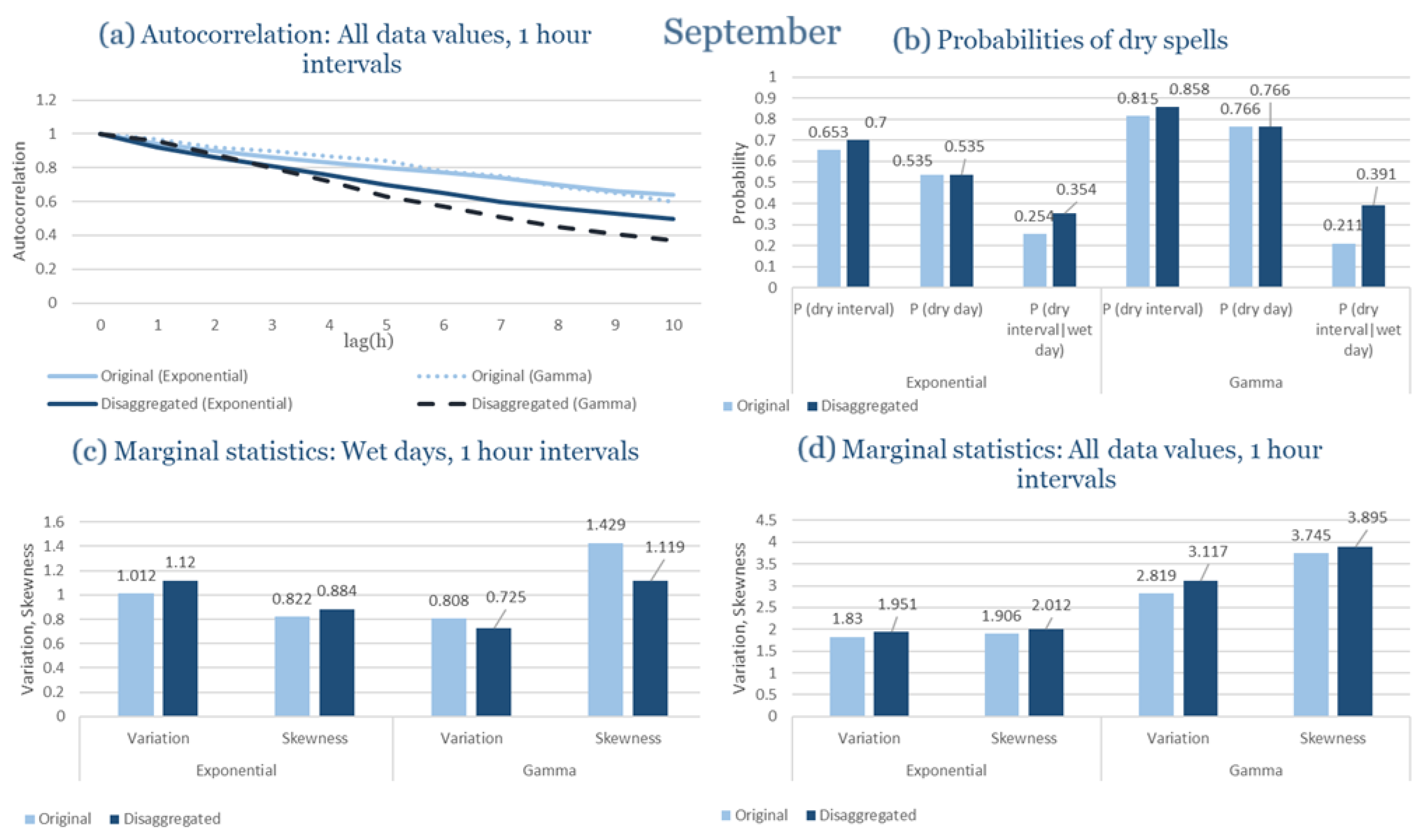
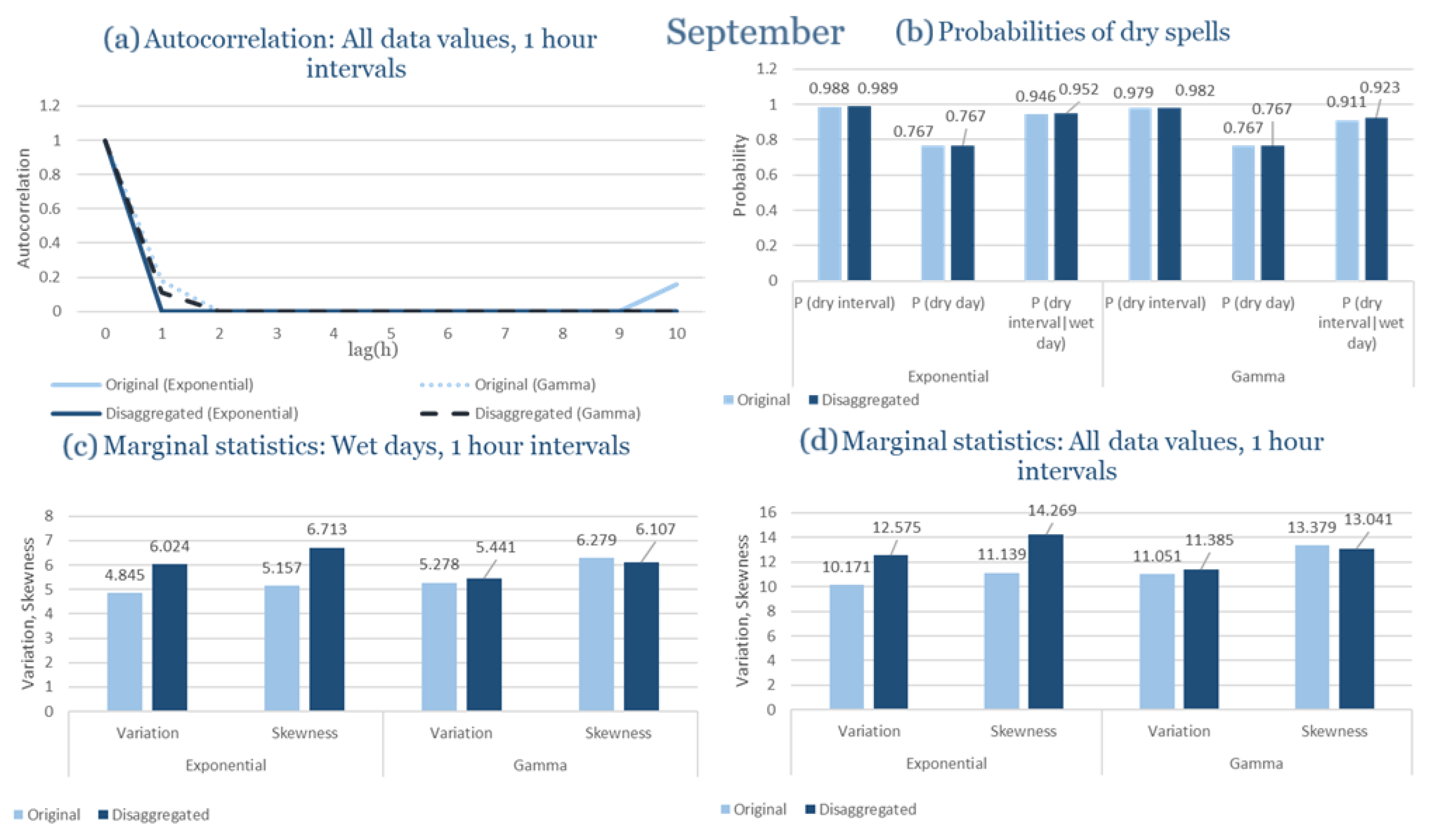
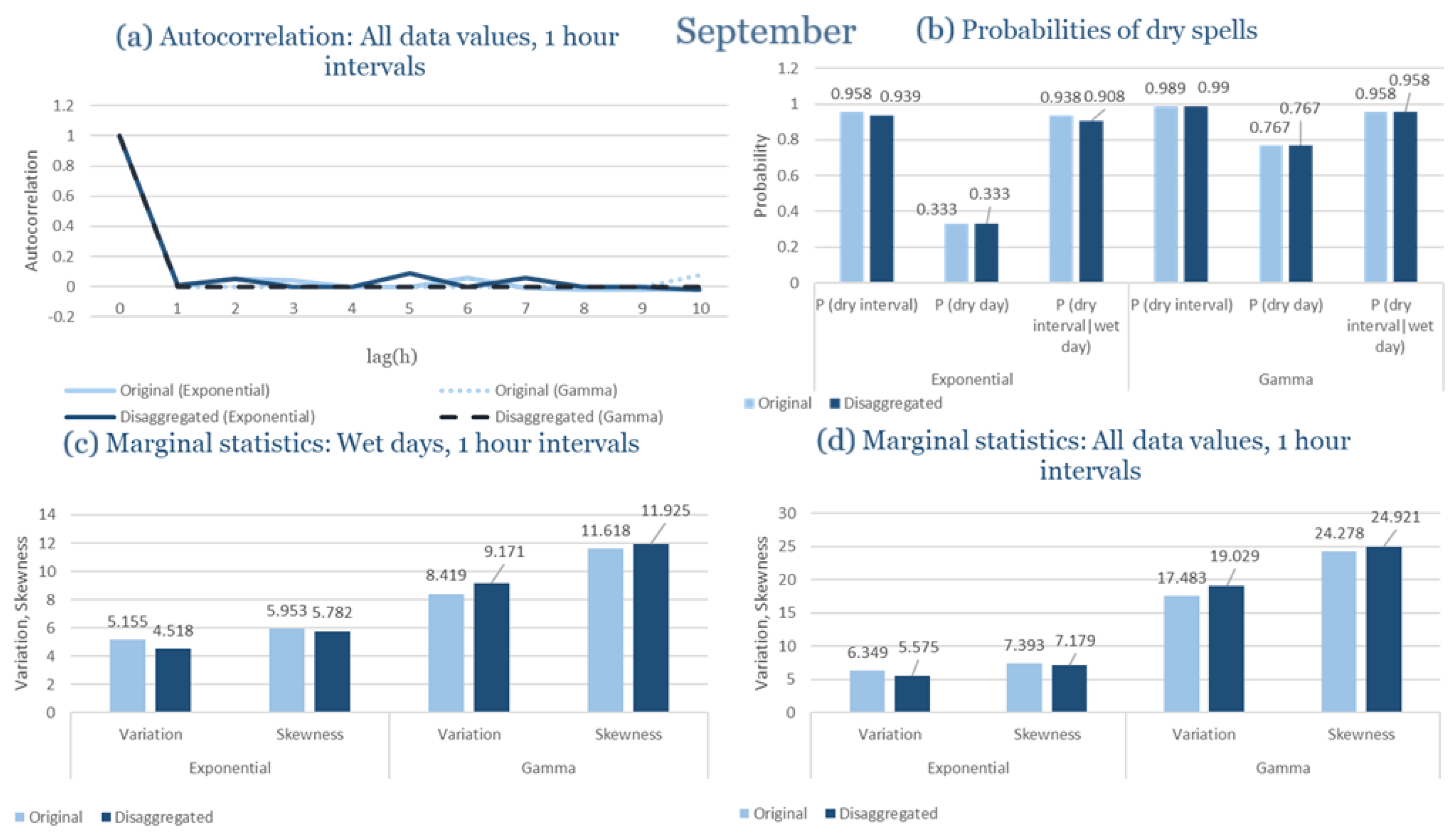
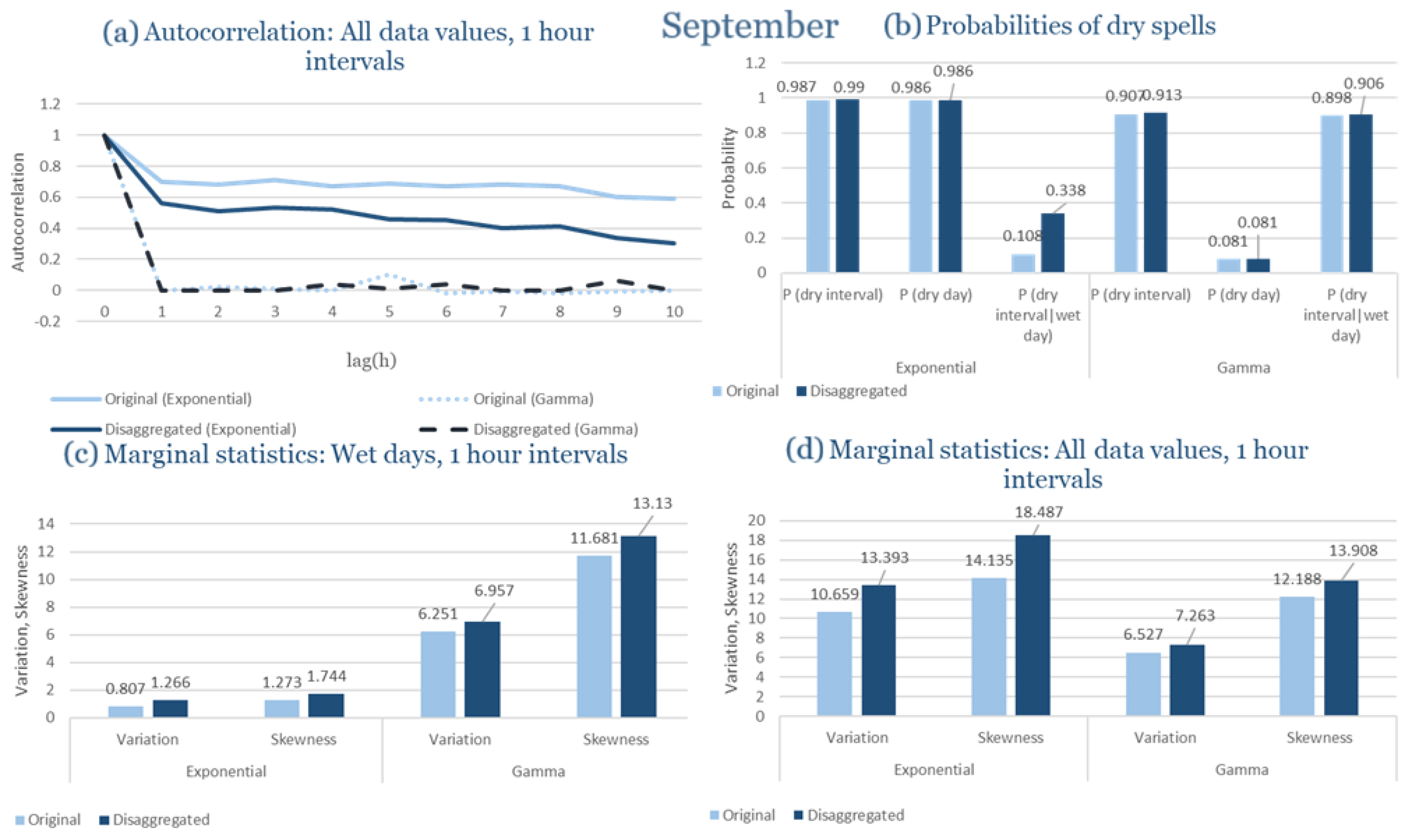
Statistical Characteristics of Corfu for September, with the intensity of the pulses following both distributions, where: (a) the diagram of the autocorrelation coefficient, (b) the diagrams of the probability of dry during a dry hour, a dry day and a dry hour||rainy day respectively, (c) the plots for the coefficient of variation and the coefficient of skewness of rainy days and (d) the plots for the coefficient of variation and the coefficient skewness for all data of the respective disagreggated time series.
Figure A22.
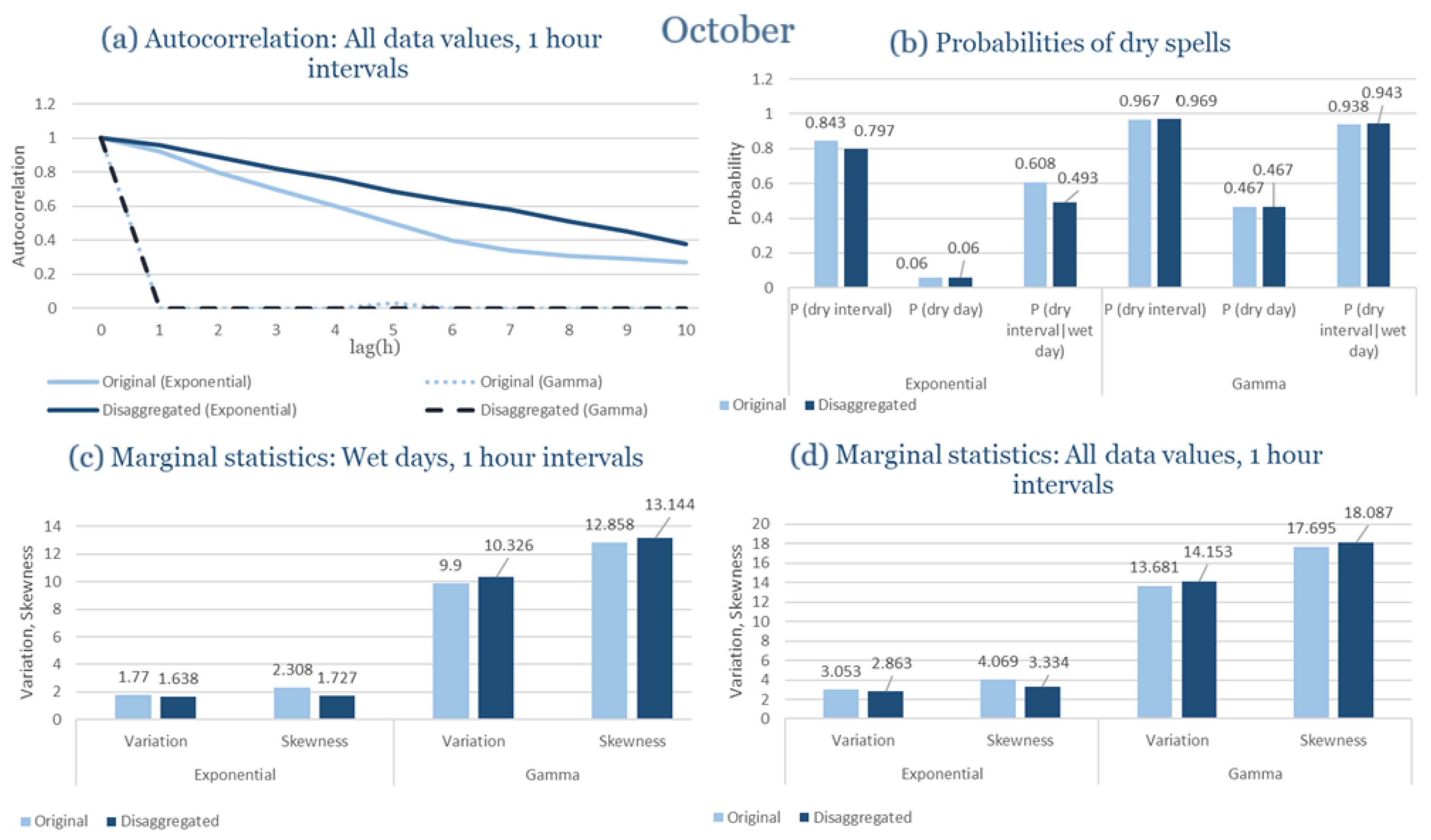
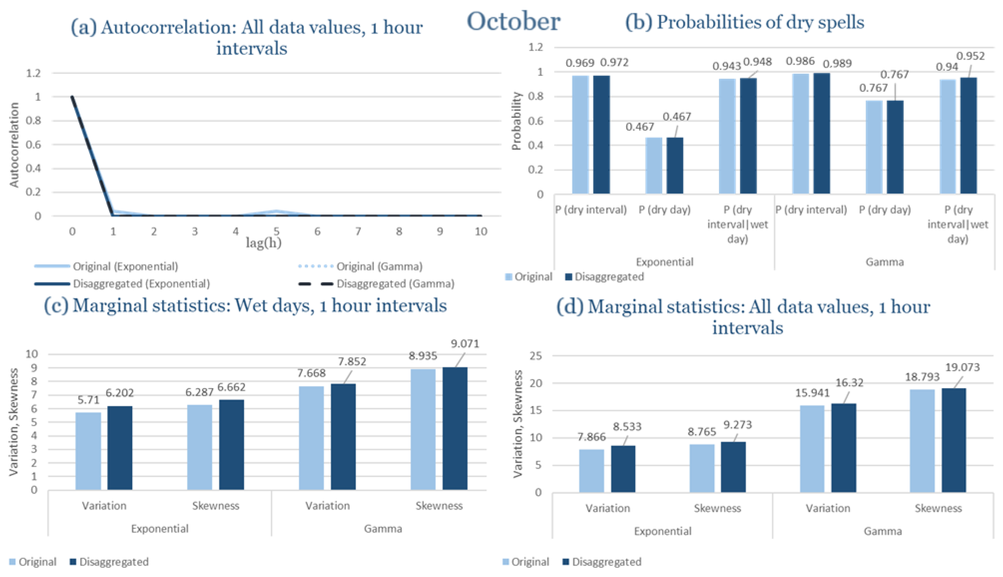
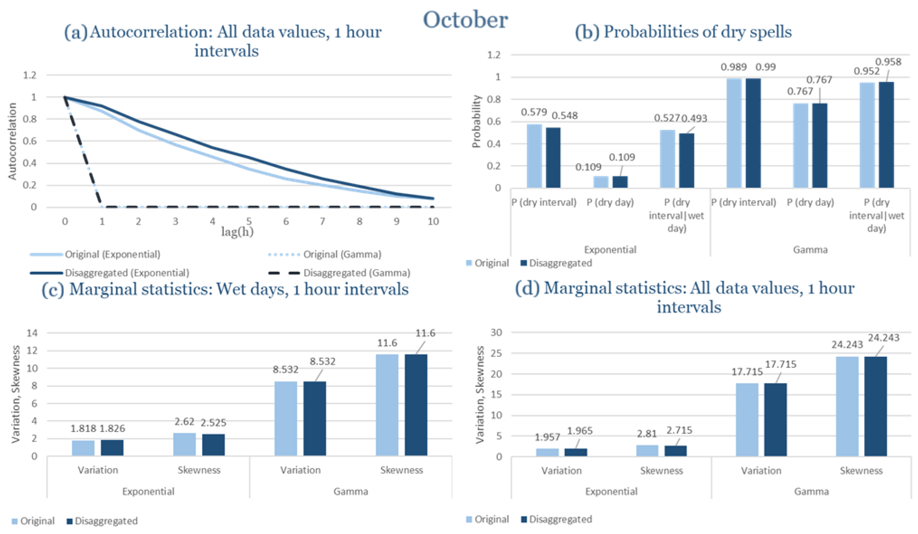
Statistical Characteristics of Corfu for October, with the intensity of the pulses following both distributions, where: (a) the diagram of the autocorrelation coefficient, (b) the diagrams of the probability of dry during a dry hour, a dry day and a dry hour||rainy day respectively, (c) the plots for the coefficient of variation and the coefficient of skewness of rainy days and (d) the plots for the coefficient of variation and the coefficient skewness for all data of the respective disagreggated time series.
Figure A23.
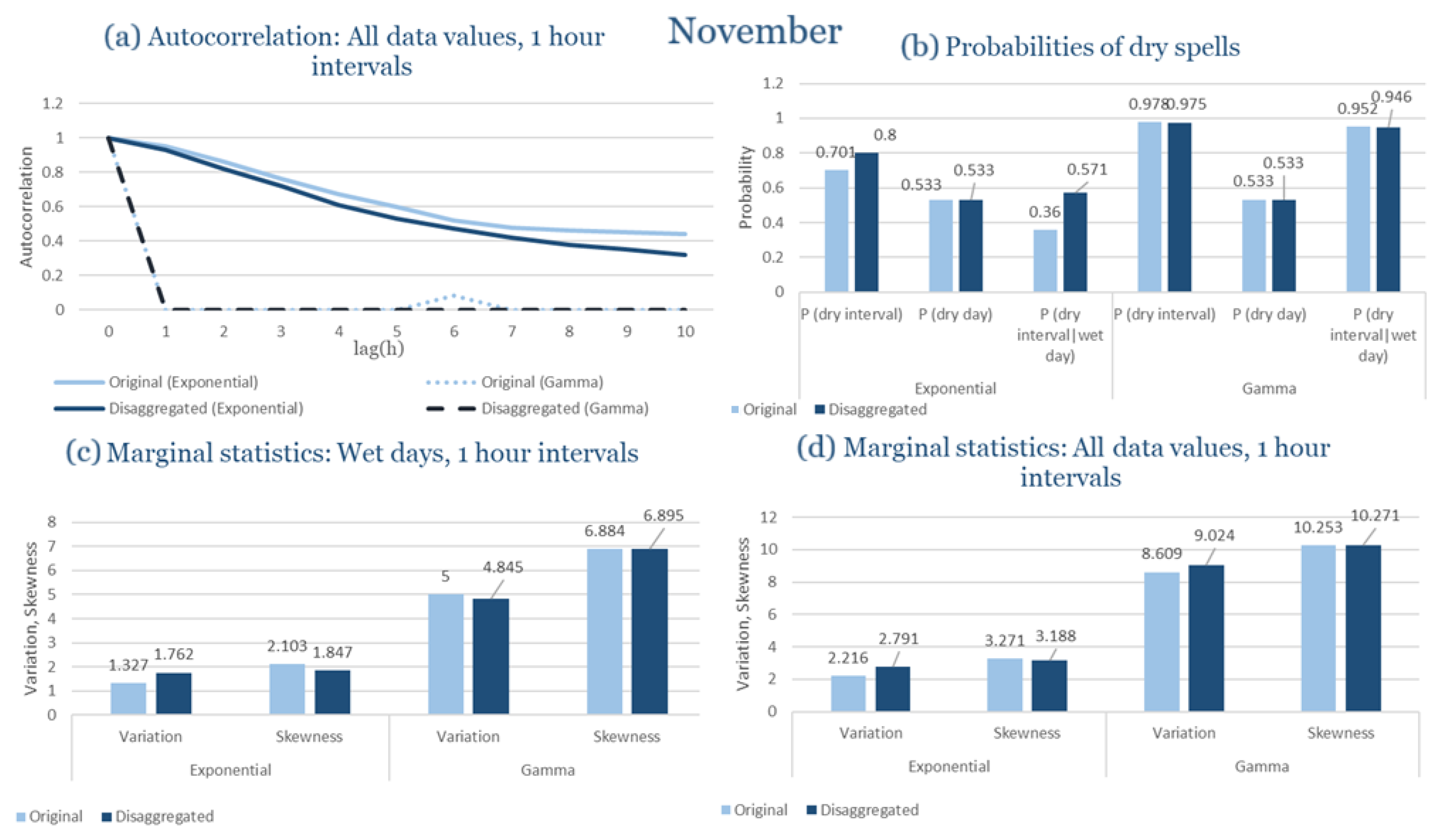
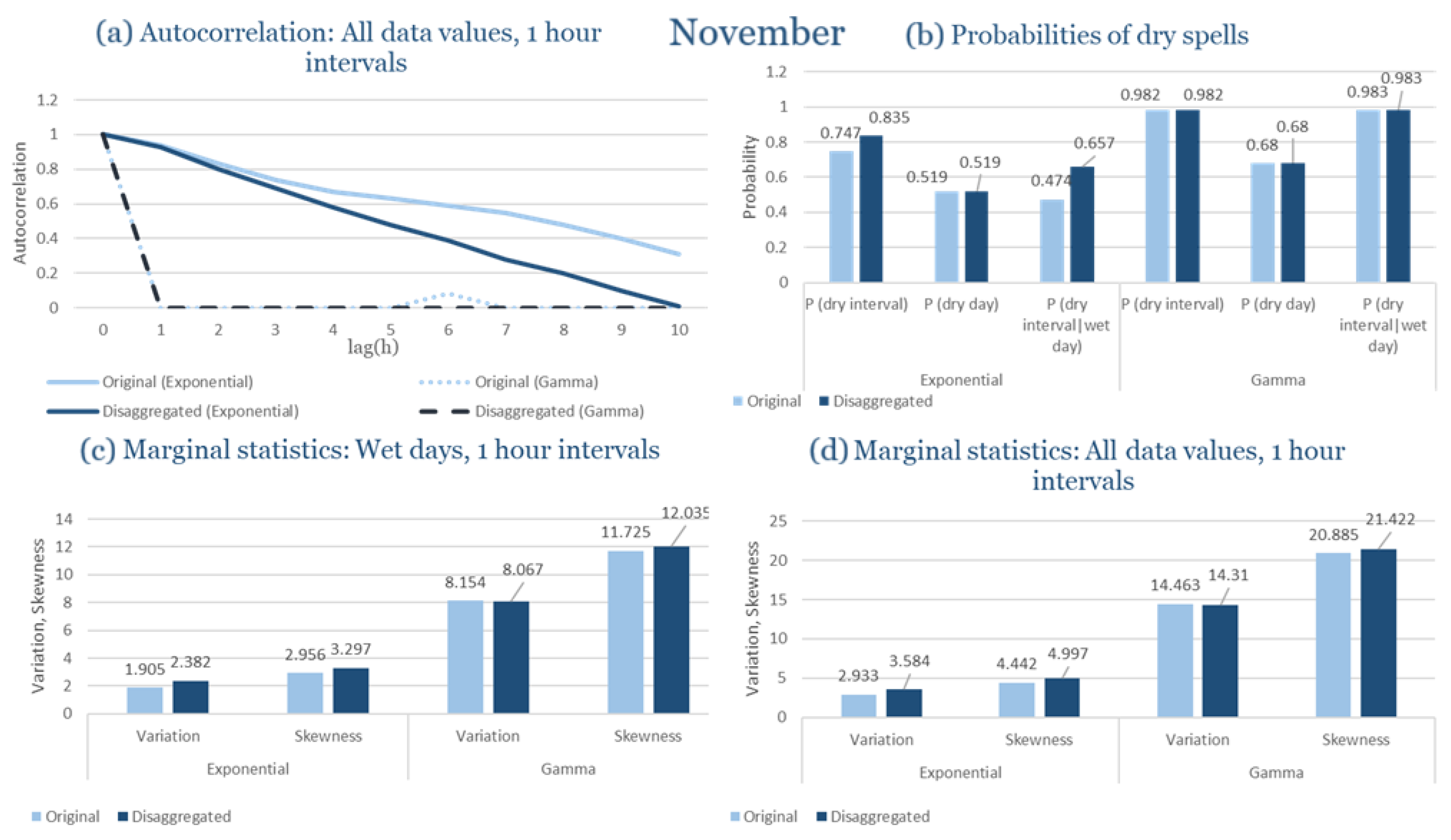
Statistical Characteristics of Corfu for November, with the intensity of the pulses following both distributions, where: (a) the diagram of the autocorrelation coefficient, (b) the diagrams of the probability of dry during a dry hour, a dry day and a dry hour||rainy day respectively, (c) the plots for the coefficient of variation and the coefficient of skewness of rainy days and (d) the plots for the coefficient of variation and the coefficient skewness for all data of the respective disagreggated time series.
Figure A24.
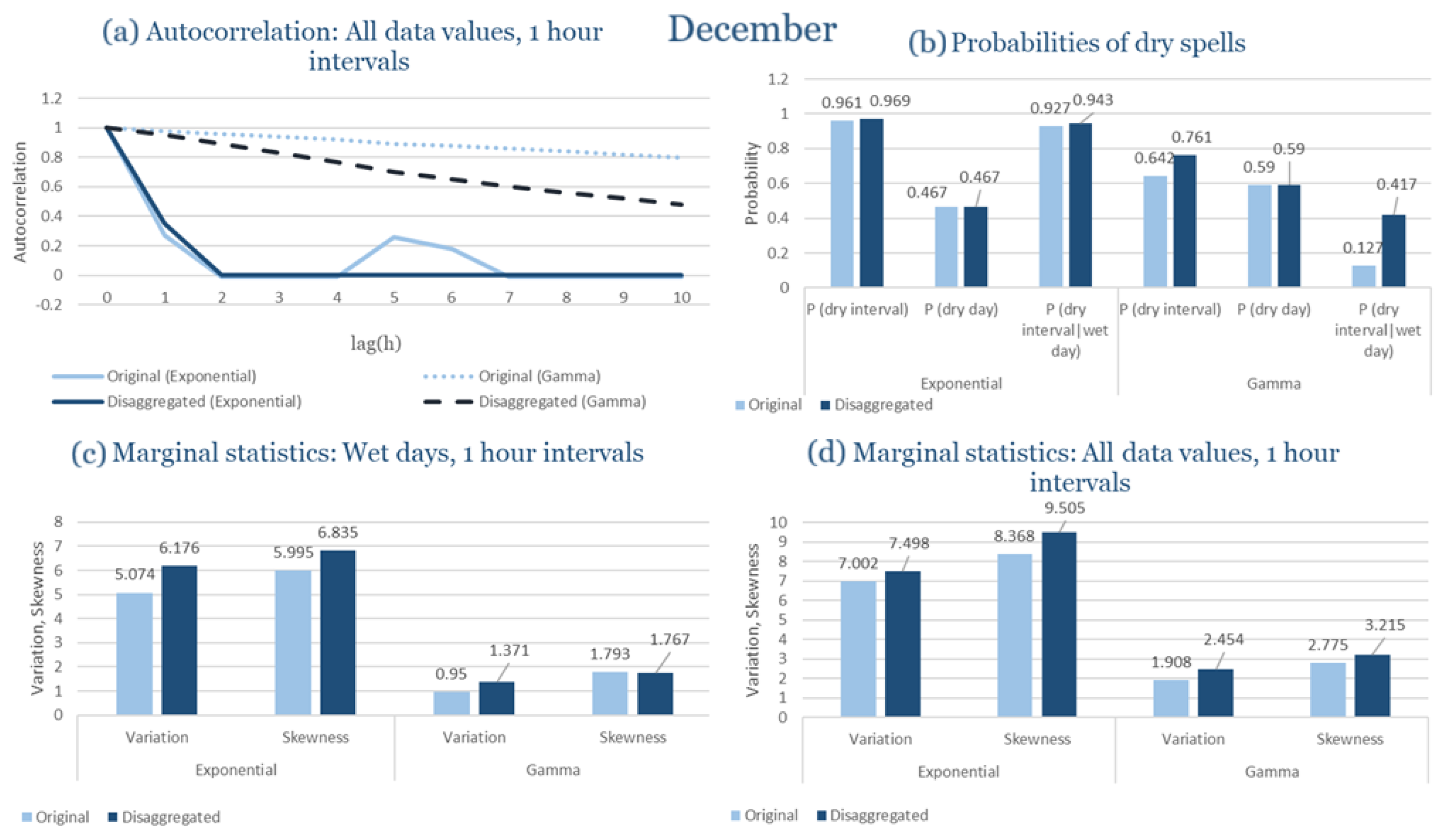
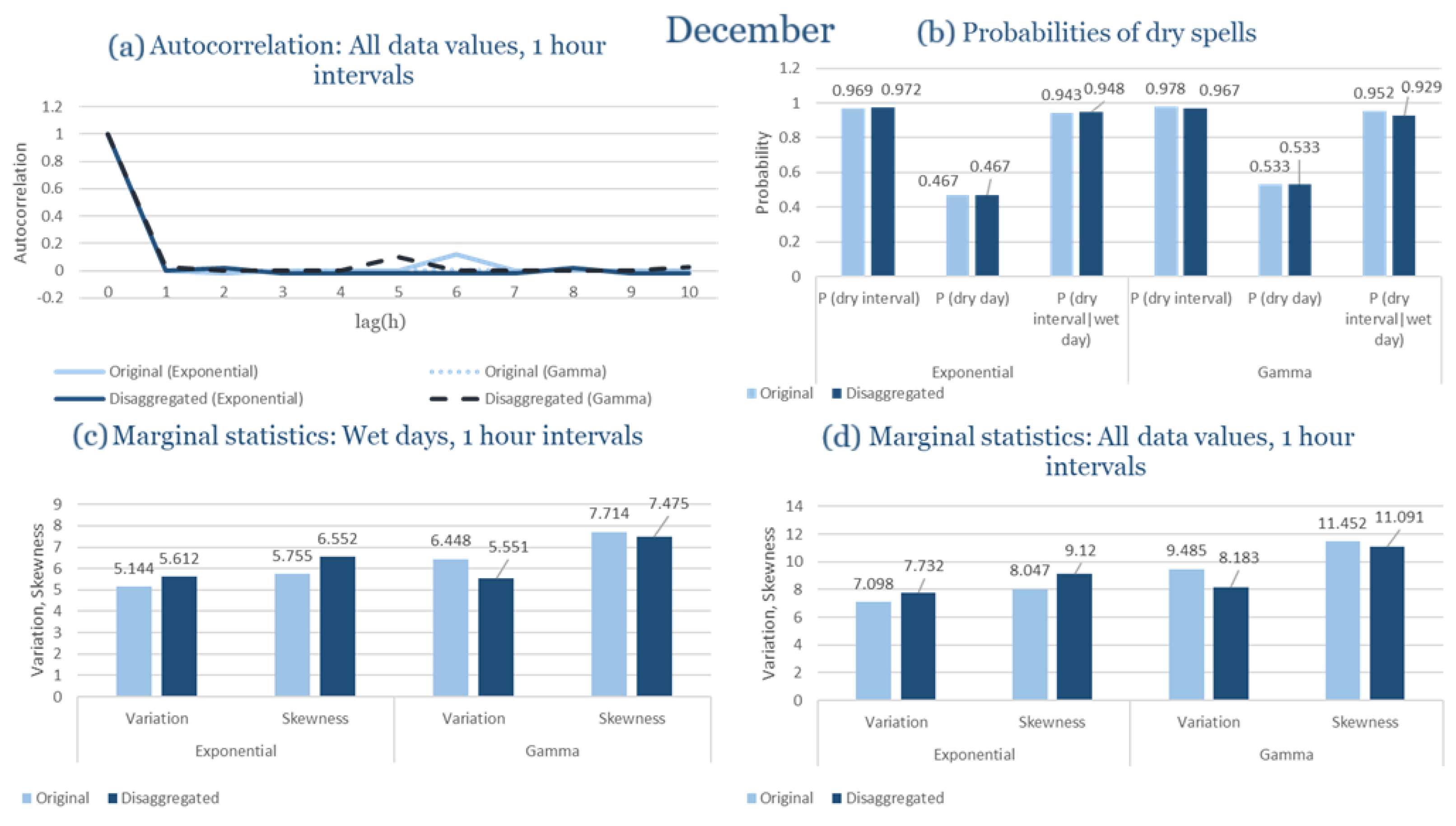
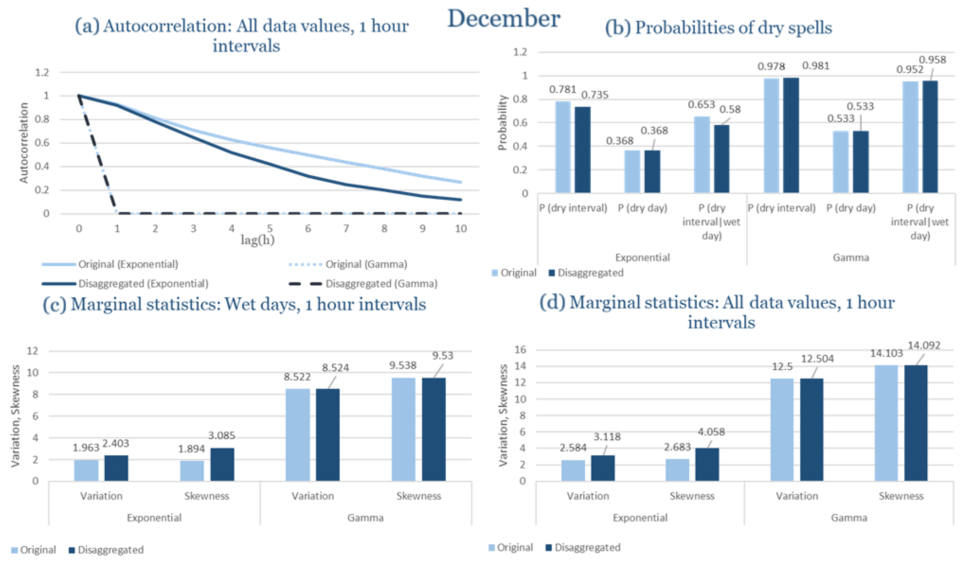
Statistical Characteristics of Corfu for December, with the intensity of the pulses following both distributions, where: (a) the diagram of the autocorrelation coefficient, (b) the diagrams of the probability of dry during a dry hour, a dry day and a dry hour||rainy day respectively, (c) the plots for the coefficient of variation and the coefficient of skewness of rainy days and (d) the plots for the coefficient of variation and the coefficient skewness for all data of the respective disagreggated time series.
Figure A25.
Statistical Characteristics of Rhodes for January, with the intensity of the pulses following both distributions, where: (a) the diagram of the autocorrelation coefficient, (b) the diagram of the probability of dry and (c) the diagrams for the coefficient of variation and skewness of the historical and synthetic timeseries.
Figure A26.
Statistical Characteristics of Rhodes for February, with the intensity of the pulses following both distributions, where: (a) the diagram of the autocorrelation coefficient, (b) the diagram of the probability of dry and (c) the diagrams for the coefficient of variation and skewness of the historical and synthetic timeseries.
Figure A27.
Statistical Characteristics of Rhodes for March, with the intensity of the pulses following both distributions, where: (a) the diagram of the autocorrelation coefficient, (b) the diagram of the probability of dry and (c) the diagrams for the coefficient of variation and skewness of the historical and synthetic timeseries.
Figure A28.
Statistical Characteristics of Rhodes for April, with the intensity of the pulses following both distributions, where: (a) the diagram of the autocorrelation coefficient, (b) the diagram of the probability of dry and (c) the diagrams for the coefficient of variation and skewness of the historical and synthetic timeseries.
Figure A29.
Statistical Characteristics of Rhodes for May, with the intensity of the pulses following both distributions, where: (a) the diagram of the autocorrelation coefficient, (b) the diagram of the probability of dry and (c) the diagrams for the coefficient of variation and skewness of the historical and synthetic timeseries.
Figure A30.
Statistical Characteristics of Rhodes for August, with the intensity of the pulses following both distributions, where: (a) the diagram of the autocorrelation coefficient, (b) the diagram of the probability of dry and (c) the diagrams for the coefficient of variation and skewness of the historical and synthetic timeseries.
Figure A31.
Statistical Characteristics of Rhodes for Septemebr, with the intensity of the pulses following both distributions, where: (a) the diagram of the autocorrelation coefficient, (b) the diagram of the probability of dry and (c) the diagrams for the coefficient of variation and skewness of the historical and synthetic timeseries.
Figure A32.
Statistical Characteristics of Rhodes for October, with the intensity of the pulses following both distributions, where: (a) the diagram of the autocorrelation coefficient, (b) the diagram of the probability of dry and (c) the diagrams for the coefficient of variation and skewness of the historical and synthetic timeseries.
Figure A33.
Statistical Characteristics of Rhodes for November, with the intensity of the pulses following both distributions, where: (a) the diagram of the autocorrelation coefficient, (b) the diagram of the probability of dry and (c) the diagrams for the coefficient of variation and skewness of the historical and synthetic timeseries.
Figure A34.
Statistical Characteristics of Rhodes for December, with the intensity of the pulses following both distributions, where: (a) the diagram of the autocorrelation coefficient, (b) the diagram of the probability of dry and (c) the diagrams for the coefficient of variation and skewness of the historical and synthetic timeseries.
Figure A35.
Statistical Characteristics of Rhodes for January, with the intensity of the pulses following both distributions, where: (a) the diagram of the autocorrelation coefficient, (b) the diagrams of the probability of dry during a dry hour, a dry day and a dry hour||rainy day respectively, (c) the plots for the coefficient of variation and the coefficient of skewness of rainy days and (d) the plots for the coefficient of variation and the coefficient skewness for all data of the respective disagreggated time series.
Figure A36.
Statistical Characteristics of Rhodes for February, with the intensity of the pulses following both distributions, where: (a) the diagram of the autocorrelation coefficient, (b) the diagrams of the probability of dry during a dry hour, a dry day and a dry hour||rainy day respectively, (c) the plots for the coefficient of variation and the coefficient of skewness of rainy days and (d) the plots for the coefficient of variation and the coefficient skewness for all data of the respective disagreggated time series.
Figure A37.
Statistical Characteristics of Rhodes for March, with the intensity of the pulses following both distributions, where: (a) the diagram of the autocorrelation coefficient, (b) the diagrams of the probability of dry during a dry hour, a dry day and a dry hour||rainy day respectively, (c) the plots for the coefficient of variation and the coefficient of skewness of rainy days and (d) the plots for the coefficient of variation and the coefficient skewness for all data of the respective disagreggated time series.
Figure A38.
Statistical Characteristics of Rhodes for April, with the intensity of the pulses following both distributions, where: (a) the diagram of the autocorrelation coefficient, (b) the diagrams of the probability of dry during a dry hour, a dry day and a dry hour||rainy day respectively, (c) the plots for the coefficient of variation and the coefficient of skewness of rainy days and (d) the plots for the coefficient of variation and the coefficient skewness for all data of the respective disagreggated time series.
Figure A39.
Statistical Characteristics of Rhodes for May, with the intensity of the pulses following both distributions, where: (a) the diagram of the autocorrelation coefficient, (b) the diagrams of the probability of dry during a dry hour, a dry day and a dry hour||rainy day respectively, (c) the plots for the coefficient of variation and the coefficient of skewness of rainy days and (d) the plots for the coefficient of variation and the coefficient skewness for all data of the respective disagreggated time series.
Figure A40.
Statistical Characteristics of Rhodes for August, with the intensity of the pulses following both distributions, where: (a) the diagram of the autocorrelation coefficient, (b) the diagrams of the probability of dry during a dry hour, a dry day and a dry hour||rainy day respectively, (c) the plots for the coefficient of variation and the coefficient of skewness of rainy days and (d) the plots for the coefficient of variation and the coefficient skewness for all data of the respective disagreggated time series.
Figure A41.
Statistical Characteristics of Rhodes for September, with the intensity of the pulses following both distributions, where: (a) the diagram of the autocorrelation coefficient, (b) the diagrams of the probability of dry during a dry hour, a dry day and a dry hour||rainy day respectively, (c) the plots for the coefficient of variation and the coefficient of skewness of rainy days and (d) the plots for the coefficient of variation and the coefficient skewness for all data of the respective disagreggated time series.
Figure A42.
Statistical Characteristics of Rhodes for October, with the intensity of the pulses following both distributions, where: (a) the diagram of the autocorrelation coefficient, (b) the diagrams of the probability of dry during a dry hour, a dry day and a dry hour||rainy day respectively, (c) the plots for the coefficient of variation and the coefficient of skewness of rainy days and (d) the plots for the coefficient of variation and the coefficient skewness for all data of the respective disagreggated time series.
Figure A43.
Statistical Characteristics of Rhodes for Novemebr, with the intensity of the pulses following both distributions, where: (a) the diagram of the autocorrelation coefficient, (b) the diagrams of the probability of dry during a dry hour, a dry day and a dry hour||rainy day respectively, (c) the plots for the coefficient of variation and the coefficient of skewness of rainy days and (d) the plots for the coefficient of variation and the coefficient skewness for all data of the respective disagreggated time series.
Figure A44.
Statistical Characteristics of Rhodes for December, with the intensity of the pulses following both distributions, where: (a) the diagram of the autocorrelation coefficient, (b) the diagrams of the probability of dry during a dry hour, a dry day and a dry hour||rainy day respectively, (c) the plots for the coefficient of variation and the coefficient of skewness of rainy days and (d) the plots for the coefficient of variation and the coefficient skewness for all data of the respective disagreggated time series.
Figure A45.
Statistical Characteristics of Alexandroupolis for January, with the intensity of the pulses following both distributions, where: (a) the diagram of the autocorrelation coefficient, (b) the diagram of the probability of dry and (c) the diagrams for the coefficient of variation and skewness of the historical and synthetic timeseries.
Figure A46.
Statistical Characteristics of Alexandroupolis for February, with the intensity of the pulses following both distributions, where: (a) the diagram of the autocorrelation coefficient, (b) the diagram of the probability of dry and (c) the diagrams for the coefficient of variation and skewness of the historical and synthetic timeseries.
Figure A47.
Statistical Characteristics of Alexandroupolis for March, with the intensity of the pulses following both distributions, where: (a) the diagram of the autocorrelation coefficient, (b) the diagram of the probability of dry and (c) the diagrams for the coefficient of variation and skewness of the historical and synthetic timeseries.
Figure A48.
Statistical Characteristics of Alexandroupolis for April, with the intensity of the pulses following both distributions, where: (a) the diagram of the autocorrelation coefficient, (b) the diagram of the probability of dry and (c) the diagrams for the coefficient of variation and skewness of the historical and synthetic timeseries.
Figure A49.
Statistical Characteristics of Alexandroupolis for May, with the intensity of the pulses following both distributions, where: (a) the diagram of the autocorrelation coefficient, (b) the diagram of the probability of dry and (c) the diagrams for the coefficient of variation and skewness of the historical and synthetic timeseries.
Figure A50.
Statistical Characteristics of Alexandroupolis for June, with the intensity of the pulses following both distributions, where: (a) the diagram of the autocorrelation coefficient, (b) the diagram of the probability of dry and (c) the diagrams for the coefficient of variation and skewness of the historical and synthetic timeseries.
Figure A51.
Statistical Characteristics of Alexandroupolis for July, with the intensity of the pulses following both distributions, where: (a) the diagram of the autocorrelation coefficient, (b) the diagram of the probability of dry and (c) the diagrams for the coefficient of variation and skewness of the historical and synthetic timeseries.
Figure A52.
Statistical Characteristics of Alexandroupolis for August, with the intensity of the pulses following both distributions, where: (a) the diagram of the autocorrelation coefficient, (b) the diagram of the probability of dry and (c) the diagrams for the coefficient of variation and skewness of the historical and synthetic timeseries.
Figure A53.
Statistical Characteristics of Alexandroupolis for September, with the intensity of the pulses following both distributions, where: (a) the diagram of the autocorrelation coefficient, (b) the diagram of the probability of dry and (c) the diagrams for the coefficient of variation and skewness of the historical and synthetic timeseries.
Figure A54.
Statistical Characteristics of Alexandroupolis for October, with the intensity of the pulses following both distributions, where: (a) the diagram of the autocorrelation coefficient, (b) the diagram of the probability of dry and (c) the diagrams for the coefficient of variation and skewness of the historical and synthetic timeseries.
Figure A55.
Statistical Characteristics of Alexandroupolis for November, with the intensity of the pulses following both distributions, where: (a) the diagram of the autocorrelation coefficient, (b) the diagram of the probability of dry and (c) the diagrams for the coefficient of variation and skewness of the historical and synthetic timeseries.
Figure A56.
Statistical Characteristics of Alexandroupolis for December, with the intensity of the pulses following both distributions, where: (a) the diagram of the autocorrelation coefficient, (b) the diagram of the probability of dry and (c) the diagrams for the coefficient of variation and skewness of the historical and synthetic timeseries.
Figure A57.
Statistical Characteristics of Alexandroupolis for January, with the intensity of the pulses following both distributions, where: (a) the diagram of the autocorrelation coefficient, (b) the diagrams of the probability of dry during a dry hour, a dry day and a dry hour||rainy day respectively, (c) the plots for the coefficient of variation and the coefficient of skewness of rainy days and (d) the plots for the coefficient of variation and the coefficient skewness for all data of the respective disagreggated time series.
Figure A58.
Statistical Characteristics of Alexandroupolis for February, with the intensity of the pulses following both distributions, where: (a) the diagram of the autocorrelation coefficient, (b) the diagrams of the probability of dry during a dry hour, a dry day and a dry hour||rainy day respectively, (c) the plots for the coefficient of variation and the coefficient of skewness of rainy days and (d) the plots for the coefficient of variation and the coefficient skewness for all data of the respective disagreggated time series.
Figure A59.
Statistical Characteristics of Alexandroupolis for March, with the intensity of the pulses following both distributions, where: (a) the diagram of the autocorrelation coefficient, (b) the diagrams of the probability of dry during a dry hour, a dry day and a dry hour||rainy day respectively, (c) the plots for the coefficient of variation and the coefficient of skewness of rainy days and (d) the plots for the coefficient of variation and the coefficient skewness for all data of the respective disagreggated time series.
Figure A60.
Statistical Characteristics of Alexandroupolis for April, with the intensity of the pulses following both distributions, where: (a) the diagram of the autocorrelation coefficient, (b) the diagrams of the probability of dry during a dry hour, a dry day and a dry hour||rainy day respectively, (c) the plots for the coefficient of variation and the coefficient of skewness of rainy days and (d) the plots for the coefficient of variation and the coefficient skewness for all data of the respective disagreggated time series.
Figure A61.
Statistical Characteristics of Alexandroupolis for May, with the intensity of the pulses following both distributions, where: (a) the diagram of the autocorrelation coefficient, (b) the diagrams of the probability of dry during a dry hour, a dry day and a dry hour||rainy day respectively, (c) the plots for the coefficient of variation and the coefficient of skewness of rainy days and (d) the plots for the coefficient of variation and the coefficient skewness for all data of the respective disagreggated time series.
Figure A62.
Statistical Characteristics of Alexandroupolis for June, with the intensity of the pulses following both distributions, where: (a) the diagram of the autocorrelation coefficient, (b) the diagrams of the probability of dry during a dry hour, a dry day and a dry hour||rainy day respectively, (c) the plots for the coefficient of variation and the coefficient of skewness of rainy days and (d) the plots for the coefficient of variation and the coefficient skewness for all data of the respective disagreggated time series.
Figure A63.
Statistical Characteristics of Alexandroupolis for July, with the intensity of the pulses following both distributions, where: (a) the diagram of the autocorrelation coefficient, (b) the diagrams of the probability of dry during a dry hour, a dry day and a dry hour||rainy day respectively, (c) the plots for the coefficient of variation and the coefficient of skewness of rainy days and (d) the plots for the coefficient of variation and the coefficient skewness for all data of the respective disagreggated time series.
Figure A64.
Statistical Characteristics of Alexandroupolis for August, with the intensity of the pulses following both distributions, where: (a) the diagram of the autocorrelation coefficient, (b) the diagrams of the probability of dry during a dry hour, a dry day and a dry hour||rainy day respectively, (c) the plots for the coefficient of variation and the coefficient of skewness of rainy days and (d) the plots for the coefficient of variation and the coefficient skewness for all data of the respective disagreggated time series.
Figure A65.
Statistical Characteristics of Alexandroupolis for September, with the intensity of the pulses following both distributions, where: (a) the diagram of the autocorrelation coefficient, (b) the diagrams of the probability of dry during a dry hour, a dry day and a dry hour||rainy day respectively, (c) the plots for the coefficient of variation and the coefficient of skewness of rainy days and (d) the plots for the coefficient of variation and the coefficient skewness for all data of the respective disagreggated time series.
Figure A66.
Statistical Characteristics of Alexandroupolis for October, with the intensity of the pulses following both distributions, where: (a) the diagram of the autocorrelation coefficient, (b) the diagrams of the probability of dry during a dry hour, a dry day and a dry hour||rainy day respectively, (c) the plots for the coefficient of variation and the coefficient of skewness of rainy days and (d) the plots for the coefficient of variation and the coefficient skewness for all data of the respective disagreggated time series.
Figure A67.
Statistical Characteristics of Alexandroupolis for November, with the intensity of the pulses following both distributions, where: (a) the diagram of the autocorrelation coefficient, (b) the diagrams of the probability of dry during a dry hour, a dry day and a dry hour||rainy day respectively, (c) the plots for the coefficient of variation and the coefficient of skewness of rainy days and (d) the plots for the coefficient of variation and the coefficient skewness for all data of the respective disagreggated time series.
Figure A68.
Statistical Characteristics of Alexandroupolis for December, with the intensity of the pulses following both distributions, where: (a) the diagram of the autocorrelation coefficient, (b) the diagrams of the probability of dry during a dry hour, a dry day and a dry hour||rainy day respectively, (c) the plots for the coefficient of variation and the coefficient of skewness of rainy days and (d) the plots for the coefficient of variation and the coefficient skewness for all data of the respective disagreggated time series.
Figure A69.
Statistical Characteristics of Herakleion for January, with the intensity of the pulses following both distributions, where: (a) the diagram of the autocorrelation coefficient, (b) the diagram of the probability of dry and (c) the diagrams for the coefficient of variation and skewness of the historical and synthetic timeseries.
Figure A70.
Statistical Characteristics of Herakleion for February, with the intensity of the pulses following both distributions, where: (a) the diagram of the autocorrelation coefficient, (b) the diagram of the probability of dry and (c) the diagrams for the coefficient of variation and skewness of the historical and synthetic timeseries.
Figure A71.
Statistical Characteristics of Herakleion for March, with the intensity of the pulses following both distributions, where: (a) the diagram of the autocorrelation coefficient, (b) the diagram of the probability of dry and (c) the diagrams for the coefficient of variation and skewness of the historical and synthetic timeseries.
Figure A72.
Statistical Characteristics of Herakleion for April, with the intensity of the pulses following both distributions, where: (a) the diagram of the autocorrelation coefficient, (b) the diagram of the probability of dry and (c) the diagrams for the coefficient of variation and skewness of the historical and synthetic timeseries.
Figure A73.
Statistical Characteristics of Herakleion for May, with the intensity of the pulses following both distributions, where: (a) the diagram of the autocorrelation coefficient, (b) the diagram of the probability of dry and (c) the diagrams for the coefficient of variation and skewness of the historical and synthetic timeseries.
Figure A74.
Statistical Characteristics of Herakleion for June, with the intensity of the pulses following both distributions, where: (a) the diagram of the autocorrelation coefficient, (b) the diagram of the probability of dry and (c) the diagrams for the coefficient of variation and skewness of the historical and synthetic timeseries.
Figure A75.
Statistical Characteristics of Herakleion for July, with the intensity of the pulses following both distributions, where: (a) the diagram of the autocorrelation coefficient, (b) the diagram of the probability of dry and (c) the diagrams for the coefficient of variation and skewness of the historical and synthetic timeseries.
Figure A76.
Statistical Characteristics of Herakleion for August, with the intensity of the pulses following both distributions, where: (a) the diagram of the autocorrelation coefficient, (b) the diagram of the probability of dry and (c) the diagrams for the coefficient of variation and skewness of the historical and synthetic timeseries.
Figure A77.
Statistical Characteristics of Herakleion for September, with the intensity of the pulses following both distributions, where: (a) the diagram of the autocorrelation coefficient, (b) the diagram of the probability of dry and (c) the diagrams for the coefficient of variation and skewness of the historical and synthetic timeseries.
Figure A78.
Statistical Characteristics of Herakleion for October, with the intensity of the pulses following both distributions, where: (a) the diagram of the autocorrelation coefficient, (b) the diagram of the probability of dry and (c) the diagrams for the coefficient of variation and skewness of the historical and synthetic timeseries.
Figure A79.
Statistical Characteristics of Herakleion for November, with the intensity of the pulses following both distributions, where: (a) the diagram of the autocorrelation coefficient, (b) the diagram of the probability of dry and (c) the diagrams for the coefficient of variation and skewness of the historical and synthetic timeseries.
Figure A80.
Statistical Characteristics of Herakleion for December, with the intensity of the pulses following both distributions, where: (a) the diagram of the autocorrelation coefficient, (b) the diagram of the probability of dry and (c) the diagrams for the coefficient of variation and skewness of the historical and synthetic timeseries.
Figure A81.
Statistical Characteristics of Herakleion for January, with the intensity of the pulses following both distributions, where: (a) the diagram of the autocorrelation coefficient, (b) the diagrams of the probability of dry during a dry hour, a dry day and a dry hour||rainy day respectively, (c) the plots for the coefficient of variation and the coefficient of skewness of rainy days and (d) the plots for the coefficient of variation and the coefficient skewness for all data of the respective disagreggated time series.
Figure A82.
Statistical Characteristics of Herakleion for February, with the intensity of the pulses following both distributions, where: (a) the diagram of the autocorrelation coefficient, (b) the diagrams of the probability of dry during a dry hour, a dry day and a dry hour||rainy day respectively, (c) the plots for the coefficient of variation and the coefficient of skewness of rainy days and (d) the plots for the coefficient of variation and the coefficient skewness for all data of the respective disagreggated time series.
Figure A83.
Statistical Characteristics of Herakleion for March, with the intensity of the pulses following both distributions, where: (a) the diagram of the autocorrelation coefficient, (b) the diagrams of the probability of dry during a dry hour, a dry day and a dry hour||rainy day respectively, (c) the plots for the coefficient of variation and the coefficient of skewness of rainy days and (d) the plots for the coefficient of variation and the coefficient skewness for all data of the respective disagreggated time series.
Figure A84.
Statistical Characteristics of Herakleion for April, with the intensity of the pulses following both distributions, where: (a) the diagram of the autocorrelation coefficient, (b) the diagrams of the probability of dry during a dry hour, a dry day and a dry hour||rainy day respectively, (c) the plots for the coefficient of variation and the coefficient of skewness of rainy days and (d) the plots for the coefficient of variation and the coefficient skewness for all data of the respective disagreggated time series.
Figure A85.
Statistical Characteristics of Herakleion for May, with the intensity of the pulses following both distributions, where: (a) the diagram of the autocorrelation coefficient, (b) the diagrams of the probability of dry during a dry hour, a dry day and a dry hour||rainy day respectively, (c) the plots for the coefficient of variation and the coefficient of skewness of rainy days and (d) the plots for the coefficient of variation and the coefficient skewness for all data of the respective disagreggated time series.
Figure A86.
Statistical Characteristics of Herakleion for June, with the intensity of the pulses following both distributions, where: (a) the diagram of the autocorrelation coefficient, (b) the diagrams of the probability of dry during a dry hour, a dry day and a dry hour||rainy day respectively, (c) the plots for the coefficient of variation and the coefficient of skewness of rainy days and (d) the plots for the coefficient of variation and the coefficient skewness for all data of the respective disagreggated time series.
Figure A87.
Statistical Characteristics of Herakleion for July, with the intensity of the pulses following both distributions, where: (a) the diagram of the autocorrelation coefficient, (b) the diagrams of the probability of dry during a dry hour, a dry day and a dry hour||rainy day respectively, (c) the plots for the coefficient of variation and the coefficient of skewness of rainy days and (d) the plots for the coefficient of variation and the coefficient skewness for all data of the respective disagreggated time series.
Figure A88.
Statistical Characteristics of Herakleion for August, with the intensity of the pulses following both distributions, where: (a) the diagram of the autocorrelation coefficient, (b) the diagrams of the probability of dry during a dry hour, a dry day and a dry hour||rainy day respectively, (c) the plots for the coefficient of variation and the coefficient of skewness of rainy days and (d) the plots for the coefficient of variation and the coefficient skewness for all data of the respective disagreggated time series.
Figure A89.
Statistical Characteristics of Herakleion for September, with the intensity of the pulses following both distributions, where: (a) the diagram of the autocorrelation coefficient, (b) the diagrams of the probability of dry during a dry hour, a dry day and a dry hour||rainy day respectively, (c) the plots for the coefficient of variation and the coefficient of skewness of rainy days and (d) the plots for the coefficient of variation and the coefficient skewness for all data of the respective disagreggated time series.
Figure A90.
Statistical Characteristics of Herakleion for October, with the intensity of the pulses following both distributions, where: (a) the diagram of the autocorrelation coefficient, (b) the diagrams of the probability of dry during a dry hour, a dry day and a dry hour||rainy day respectively, (c) the plots for the coefficient of variation and the coefficient of skewness of rainy days and (d) the plots for the coefficient of variation and the coefficient skewness for all data of the respective disagreggated time series.
Figure A91.
Statistical Characteristics of Herakleion for November, with the intensity of the pulses following both distributions, where: (a) the diagram of the autocorrelation coefficient, (b) the diagrams of the probability of dry during a dry hour, a dry day and a dry hour||rainy day respectively, (c) the plots for the coefficient of variation and the coefficient of skewness of rainy days and (d) the plots for the coefficient of variation and the coefficient skewness for all data of the respective disagreggated time series.
Figure A92.
Statistical Characteristics of Herakleion for December, with the intensity of the pulses following both distributions, where: (a) the diagram of the autocorrelation coefficient, (b) the diagrams of the probability of dry during a dry hour, a dry day and a dry hour||rainy day respectively, (c) the plots for the coefficient of variation and the coefficient of skewness of rainy days and (d) the plots for the coefficient of variation and the coefficient skewness for all data of the respective disagreggated time series.
