Causal Random Forests Model Using Instrumental Variable Quantile Regression

Abstract

We propose an econometric procedure based mainly on the generalized random forests method. Not only does this process estimate the quantile treatment effect nonparametrically, but our procedure yields a measure of variable importance in terms of heterogeneity among control variables. We also apply the proposed procedure to reinvestigate the distributional effect of 401(k) participation on net financial assets, and the quantile earnings effect of participating in a job training program.

1. Introduction

Causal machine learning, which is based on two approaches: the double machine learning (DML), cf. Chernozhukov et al. (2018), and the generalized random forests method (GRF), cf. Athey et al. (2019), has been actively studied in economics in recent years. With the identification strategy of selection on observables, empirical applications have been investigated by using the aforementioned two approaches, including the works by Gilchrist and Sands (2016) and Davis and Heller (2017). When it comes to the identification strategy of selection on unobservables, few empirical papers using causal machine learning can be found in the existing literature. Those empirical applications very often lack important observed control variables or involve reverse causality, and thus researchers resort to the instrumental variable approach. Additionally, it remains unclear how the quantile treatment effect is to be estimated under the DML and GRF methods. In this paper, with the use of instrumental variables, we propose an econometric procedure for estimating quantile treatment effects based primarily on the generalized random forests of Athey et al. (2019).

Chernozhukov and Hansen (2005) propose an estimator that addresses endogeneity in quantile regressions via rank similarity, a crucial feature absent in the prior approaches. Using rank similarity, this estimator studies the heterogeneous quantile effects of an endogenous variable over the entire population (rather than for the compliers). Rank similarity thus identifies population-based quantile treatment effects, cf. Frandsen and Lefgren (2018). This approach does not require the monotonicity assumption used in Abadie et al. (2002) and allows for binary or continuous endogenous and instrumental variables. Chernozhukov and Hansen (2008) create a bridge between two-stage least squares (2SLS) estimator and their 2005 estimator, and propose an estimator robust to weak instruments. However, it is noteworthy that these estimator are unable to estimate unconditional quantiles, which are, as discussed in Guilhem et al. (2019), quantities that should be of utmost interest to empirical researchers. In this paper, we use the instrumental variable quantile regression of Chernozhukov and Hansen (2008) as a vehicle for identifying the quantile treatment effect.

Athey and Imbens (2016) is the first paper that develops the regression tree model to estimate heterogeneous treatment effects using the honest splitting algorithm. Wager and Athey (2018) extend the regression tree model to causal forests. Recently, Athey et al. (2019) have developed the generalized random forests model, which is a unified framework in the sense that it is built on local moment conditions capable of encompassing many models. Therefore, we bring the first order condition of the instrumental variable quantile regression into the local moment conditions and then modify the GRF algorithm. Accordingly, the quantile treatment effect can be estimated under the framework of causal random forests. Thus, our proposed estimator and the generalized random forests model both share the advantage of estimating the conditional quantile treatment effect nonparametrically.

Chen and Tien (2019) investigate the instrumental variable quantile regression in the context of double machine learning. Although related to their paper, our procedure is not considering the same high-dimensional setting. Further, in contrast to the DML for instrumental variable quantile regressions, the proposed econometric procedure yields a measure of variable importance in terms of heterogeneity among control variables. The pattern of variable importance across quantiles can be revealed as well. We highlight the usage of exploring variable importance by reinvestigating two empirical studies - the distributional effect of 401(k) participation on net financial assets, and the quantile effect of participating in a job training program on earnings.

The rest of the paper is organized as follows. The model specification and practical algorithm are introduced in Section 2. Section 3 presents the measure of variable importance. Section 4 presents two empirical applications. Section 5 concludes the paper. The Appendix A discusses the usage of a doubly robust method along with the causal random forests structure for achieving more efficient estimation. The Appendix A also discusses the identifying restrictions and regularity conditions for the instrumental variable quantile regression and the generalized random forests, and further verifies conditions for establishing consistency and asymptotic normality of the proposed estimator.

2. The Model and Algorithm

We propose the causal random forests with the instrumental variable quantile regression (GRF-IVQR, hereafter). Estimation procedure of the GRF-IVQR is constructed as below, essentially based on the method developed in Athey et al. (2019).

2.1. Generalized Random Forests

The classification tree and regression tree (CART) and its extension, random forests Breiman (2001), are effective methods for flexibly estimating regression functions in terms of out-of-sample predictive power. Random forests have become particularly popular methods. A key attraction is that they require relatively little tuning and have superior performance to more complex methods such as deep learning neural networks, cf. Section 3.2 of Athey and Imbens (2019). Recently, random forests have garnered interest and have been extended to causal effects; that is, the generalized random forests estimator.

In what follows, we describe how we incorporate the instrumental variable quantile regression into the framework of GRF and modify the resulting estimator accordingly.

Given data $(X_i,O_i)\in \mathcal{X}\times \mathcal{O}$, we estimate the parameter of interest $\theta \left(x\right)$ via the following moment conditions

$$\begin{array}{c}\hfill \mathbb{E}[{\psi }_{\theta \left(x\right),\nu \left(x\right)}\left(O_i\right)\mid X_i=x]=0\mathrm{for}\mathrm{all}x\in \mathcal{X},\end{array}$$

where $\psi (·)$ stands for the score function and $\nu \left(x\right)$ are optional nuisance parameters. The above moment conditions, similar to the generalized method of moments (GMM), can be used to identify many objects of interest from an economic perspective. We seek forest-based estimates, $\widehat{\theta }\left(x\right)$, which are the conditional quantile treatment effects, in the context of instrumental variable quantile regressions.

Chernozhukov and Hansen (2005) laid the theoretical foundations for the instrumental variable quantile regression (IVQR). With outcome $Y_i$, endogenous treatment variable $D_i$, instrumental variable $Z_i$, and control variables $X_i$, the IVQR can be represented as the following moment conditions

$$\begin{array}{cc}\hfill & \mathbb{E}\left[{\psi }_{\theta \left(\tau \right),\nu \left(\tau \right)}\left(Y_i\right)|\{D_i,X_i,Z_i\}\right]\hfill \\ \hfill & =\mathbb{E}\left\{\left[\tau -1\left(Y_i\le D_i\theta \left(\tau \right)+X_i\nu \left(\tau \right)\right)\right]{(Z_i,X_i)}^{\prime }|\{D_i,X_i,Z_i\}\right\},\hfill \end{array}$$

where $\theta \left(\tau \right)$ is the conditional quantile treatment effect, $\nu \left(\tau \right)$ are the nuisance parameters, $1(·)$ is the indicator function, and $\tau$ is a quantile index.

The sample counterpart of the local moment conditions and the estimator of $\theta$ are introduced by Athey et al. (2019) and defined as below.

$$\begin{array}{c}\hfill \left(\widehat{\theta }(\tau ,x),\widehat{\nu }(\tau ,x)\right)\in \underset{\theta \left(\tau \right),\nu \left(\tau \right)}{argmin}\left\{{∥\sum _{i=1}^n{\alpha }_i\left(x\right){\psi }_{\theta \left(\tau \right),\nu \left(\tau \right)}\left(Y_i\right)∥}_2\right\},\end{array}$$

where ${\alpha }_i\left(x\right)$ are tree-based weights averaged by the forest, which measure how often each training example falls in the same leaf as x. In other words, these weights represent the relevance of each sample when we estimate $\theta$. Specifically, the weights are obtained by a forest-based algorithm. For the point of interest x, let $L_b\left(x\right)$ represent the set of samples which fall in the same terminal leaf and contain x in bth tree, where $b\in \{1,2,...,B\}$. That is to say, the weight ${\alpha }_i\left(x\right)$ of each sample for the point of interest x will be the frequency with which the ith sample is in the same terminal leaf among all trees $\{1,2,...,B\}$. That is,

$$\begin{array}{cc}\hfill {\alpha }_{bi}\left(x\right)& =\frac{1(X_i\in L_b\left(x\right))}{\left|L_b\left(x\right)\right|},\hfill \\ \hfill {\alpha }_i\left(x\right)& =\frac{1}{B}\sum _{b=1}^B{\alpha }_{bi}\left(x\right).\hfill \end{array}$$

With such forest-based weights and a pre-specified quantile index $\tau$, we minimize the criterion function constructed using sample moment conditions, and then an estimate of the conditional quantile treatment effect $\widehat{\theta }\left(\tau \right)$ is obtained. In the subsequent section, we discuss how to grow the trees and the forests with the instrumental variable quantile regression.

2.2. Tree Splitting Rules

Growing a tree is a recursive binary splitting process. The spirit of the tree-based algorithm is to split the data in the parent node P in half by maximizing the heterogeneity of the associated two children nodes $\{C_1,C_2\}$.

Specifically, for node j with data $\mathcal{J}$, we define the node parameters as follows.

$$\begin{array}{c}\hfill \left({\widehat{\theta }}_j\left(\tau \right),{\widehat{\nu }}_j\left(\tau \right)\right)\left(\mathcal{J}\right)\in \underset{\theta \left(\tau \right),\nu \left(\tau \right)}{argmin}\left\{{∥\sum _{i\in \mathcal{J}:X_i\in j}{\psi }_{\theta \left(\tau \right),\nu \left(\tau \right)}\left(Y_i\right)∥}_2\right\},\end{array}$$

where $j\in \{P,C\}$. In each node, we minimize the following criterion

$$\begin{array}{c}\hfill \mathrm{err}(C_1,C_2)=\sum _{j=1,2}\mathbb{P}[X\in C_j\mid X\in P]·\mathbb{E}\left[{\left({\widehat{\theta }}_{C_j}\left(\tau \right)-\theta (\tau ,X)\right)}^2|X\in C_j\right],\end{array}$$

which is based on the GRF method. However, the minimization is infeasible due to the unknown value of $\theta (\tau ,X)$. Athey et al. (2019) turn this minimization problem of $\mathrm{err}(C_1,C_2)$ into an accessible model-free maximization problem of

$$\begin{array}{c}\hfill \Delta (C_1,C_2):=\frac{n_{C_1}{n}_{C_2}}{n_P^2}{\left({\widehat{\theta }}_{C_1}\left(\tau \right)-{\widehat{\theta }}_{C_2}\left(\tau \right)\right)}^2,\end{array}$$

where $n_{C_1},n_{C_2},n_P$ are numbers of observations in children and parent nodes. Along the way of maximizing $\Delta$, the ${\theta }_{C_j}\left(\tau \right)$ is estimated by the IVQR with respect to all possible splittings which correspond to the set $\{\mathrm{all}\mathrm{possible}\mathrm{values}\mathrm{for}{X}_i,\forall i\}$. Consequently, the estimation is computationally infeasible. To circumvent this difficulty, Athey et al. (2019) suggest a gradient tree algorithm which maximizes an approximate criterion $\tilde{\Delta }(C_1,C_2)$. In what follows, with two new ingredients $A_p$ and $\rho$ defined below, we construct $\tilde{\Delta }(C_1,C_2)$ step by step.

We first define $A_p$ as the gradient of the expectation of the moment condition.

$$\begin{array}{cc}\hfill A_p& =\nabla \mathbb{E}\left[{\psi }_{{\widehat{\theta }}_P\left(\tau \right),{\widehat{\nu }}_P\left(\tau \right)}\left(Y_i\right)|\{D_i,X_i,Z_i\}\in P\right]\hfill \\ \hfill & =\nabla \mathbb{E}\left[\left(\tau -1\left(Y_i\le D_i{\widehat{\theta }}_P\left(\tau \right)+X_i{\widehat{\nu }}_P\left(\tau \right)\right)\right){(Z_i,X_i)}^{\prime }|\{D_i,X_i,Z_i\}\in P\right]\hfill \\ \hfill & =\nabla \left[\left(\tau -F\left(D_i{\widehat{\theta }}_P\left(\tau \right)+X_i{\widehat{\nu }}_P\left(\tau \right)\right)\right){(Z_i,X_i)}^{\prime }|\{D_i,X_i,Z_i\}\in P\right]\hfill \\ \hfill & =\nabla {\left[\begin{array}{c}\tau Z_i-F\left(D_i{\widehat{\theta }}_P\left(\tau \right)+X_i{\widehat{\nu }}_P\left(\tau \right)\right)Z_i\\ \tau X_{1i}-F\left(D_i{\widehat{\theta }}_P\left(\tau \right)+X_i{\widehat{\nu }}_P\left(\tau \right)\right)X_{1i}\\ ⋮\\ \tau X_{mi}-F\left(D_i{\widehat{\theta }}_P\left(\tau \right)+X_i{\widehat{\nu }}_P\left(\tau \right)\right)X_{mi}\end{array}|\{D_i,X_i,Z_i\}\in P\right]}^{\prime },\hfill \end{array}$$

where $F(·)$ is a cumulative distribution function, and m is the dimension of X. For simplicity of derivation, we fix the following notations. $g_0:=\tau Z_i-F\left(D_i{\widehat{\theta }}_P\left(\tau \right)+X_i{\widehat{\nu }}_P\left(\tau \right)\right)Z_i$, $g_1:=\tau X_{1i}-F\left(D_i{\widehat{\theta }}_P\left(\tau \right)+X_i{\widehat{\nu }}_P\left(\tau \right)\right)X_{1i}$, ⋯, $g_m:=\tau X_{mi}-F\left(D_i{\widehat{\theta }}_P\left(\tau \right)+X_i{\widehat{\nu }}_P\left(\tau \right)\right)X_{mi}$, and we suppress $[·|\{D_i,X_i,Z_i\}\in P]$ which means the estimation is conditional on the parent node. Accordingly, $A_p$ can be written as the gradient of $g_0,g_1,\cdots ,g_m$ with respect to the parent node parameters.

$$\begin{array}{cc}\hfill A_p& ={\nabla }_{{\widehat{\theta }}_P\left(\tau \right),{\widehat{\nu }}_P\left(\tau \right)}{\left[\begin{array}{c}{g}_0\\ g_1\\ ⋮\\ g_m\end{array}\right]}^{\prime }=\left[\begin{array}{ccccc}{\displaystyle \frac{\partial g_0}{\partial {\widehat{\theta }}_P\left(\tau \right)}}& {\displaystyle \frac{\partial g_1}{\partial {\widehat{\theta }}_P\left(\tau \right)}}& {\displaystyle \frac{\partial g_2}{\partial {\widehat{\theta }}_P\left(\tau \right)}}& \cdots & {\displaystyle \frac{\partial g_m}{\partial {\widehat{\theta }}_P\left(\tau \right)}}\\ {\displaystyle \frac{\partial g_0}{\partial {\widehat{\nu }}_{1,P}\left(\tau \right)}}& {\displaystyle \frac{\partial g_1}{\partial {\widehat{\nu }}_{1,P}\left(\tau \right)}}& {\displaystyle \frac{\partial g_2}{\partial {\widehat{\nu }}_{1,P}\left(\tau \right)}}& \cdots & {\displaystyle \frac{\partial g_m}{\partial {\widehat{\nu }}_{1,P}\left(\tau \right)}}\\ ⋮& ⋮& ⋮& \ddots & ⋮\\ {\displaystyle \frac{\partial g_0}{\partial {\widehat{\nu }}_{m,P}\left(\tau \right)}}& {\displaystyle \frac{\partial g_1}{\partial {\widehat{\nu }}_{m,P}\left(\tau \right)}}& {\displaystyle \frac{\partial g_2}{\partial {\widehat{\nu }}_{m,P}\left(\tau \right)}}& \cdots & {\displaystyle \frac{\partial g_m}{\partial {\widehat{\nu }}_{m,P}\left(\tau \right)}}\end{array}\right]\hfill \\ \hfill & =\left[\begin{array}{c}\hfill \begin{array}{cccc}-f\left(D_i{\widehat{\theta }}_P\left(\tau \right)+X_i{\widehat{\nu }}_P\left(\tau \right)\right)Z_i{D}_i& -f\left(D_i{\widehat{\theta }}_P\left(\tau \right)+X_i{\widehat{\nu }}_P\left(\tau \right)\right)X_{1i}{D}_i& \cdots & -f\left(D_i{\widehat{\theta }}_P\left(\tau \right)+X_i{\widehat{\nu }}_P\left(\tau \right)\right)X_{mi}{D}_i\\ -f\left(D_i{\widehat{\theta }}_P\left(\tau \right)+X_i{\widehat{\nu }}_P\left(\tau \right)\right)Z_i{X}_{1i}& -f\left(D_i{\widehat{\theta }}_P\left(\tau \right)+X_i{\widehat{\nu }}_P\left(\tau \right)\right)X_{1i}{X}_{1i}& \cdots & -f\left(D_i{\widehat{\theta }}_P\left(\tau \right)+X_i{\widehat{\nu }}_P\left(\tau \right)\right)X_{mi}{X}_{1i}\\ ⋮& ⋮& \ddots & ⋮\\ -f\left(D_i{\widehat{\theta }}_P\left(\tau \right)+X_i{\widehat{\nu }}_P\left(\tau \right)\right)Z_i{X}_{mi}& -f\left(D_i{\widehat{\theta }}_P\left(\tau \right)+X_i{\widehat{\nu }}_P\left(\tau \right)\right)X_{1i}{X}_{mi}& \cdots & -f\left(D_i{\widehat{\theta }}_P\left(\tau \right)+X_i{\widehat{\nu }}_P\left(\tau \right)\right)X_{mi}{X}_{mi}\end{array}\end{array}\right]\hfill \\ \hfill & =-f\left(D_i{\widehat{\theta }}_P\left(\tau \right)+X_i{\widehat{\nu }}_P\left(\tau \right)\right)\left[\begin{array}{cccc}{Z}_i{D}_i& X_{1i}{D}_i& \cdots & X_{mi}{D}_i\\ Z_i{X}_{1i}& X_{1i}{X}_{1i}& \cdots & X_{mi}{X}_{1i}\\ ⋮& ⋮& \ddots & ⋮\\ Z_i{X}_{mi}& X_{1i}{X}_{mi}& \cdots & X_{mi}{X}_{mi}\end{array}\right],\hfill \end{array}$$

where $f(·)$ is the probability density function of $F(·)$. Therefore, the inverse of $A_p$,

$$\begin{array}{cc}\hfill A_p^{-1}& ={\left\{-f\left(D_i{\widehat{\theta }}_P\left(\tau \right)+X_i{\widehat{\nu }}_P\left(\tau \right)\right)\left[\begin{array}{cccc}{Z}_i{D}_i& X_{1i}{D}_i& \cdots & X_{mi}{D}_i\\ Z_i{X}_{1i}& X_{1i}{X}_{1i}& \cdots & X_{mi}{X}_{1i}\\ ⋮& ⋮& \ddots & ⋮\\ Z_i{X}_{mi}& X_{1i}{X}_{mi}& \cdots & X_{mi}{X}_{mi}\end{array}\right]\right\}}^{-1}\hfill \\ \hfill & =\frac{-1}{f\left(D_i{\widehat{\theta }}_P\left(\tau \right)+X_i{\widehat{\nu }}_P\left(\tau \right)\right)}{\left[\begin{array}{cccc}{Z}_i{D}_i& X_{1i}{D}_i& \cdots & X_{mi}{D}_i\\ Z_i{X}_{1i}& X_{1i}{X}_{1i}& \cdots & X_{mi}{X}_{1i}\\ ⋮& ⋮& \ddots & ⋮\\ Z_i{X}_{mi}& X_{1i}{X}_{mi}& \cdots & X_{mi}{X}_{mi}\end{array}\right]}^{-1}.\hfill \end{array}$$

We then construct the pseudo-outcomes,

$$\begin{array}{cc}\hfill {\rho }_i& =-{\xi }^{\top }{A}_p^{-1}{\psi }_{{\widehat{\theta }}_P\left(\tau \right),{\widehat{\nu }}_P\left(\tau \right)}\left(Y_i\right),\hfill \end{array}$$

where $\xi$ is a vector that picks out the $\theta \left(\tau \right)$-coordinate from the $\left(\theta \right(\tau ),\nu (\tau \left)\right)$ vector. In the case with one treatment variable D, the $\xi$ vector is $(1,0,...,0)$. Thus, the corresponding pseudo-outcomes are

$$\begin{array}{cc}\hfill {\rho }_i& =-{\left[\begin{array}{c}1\\ 0\\ ⋮\\ 0\end{array}\right]}^{\prime }\left\{\frac{-1}{f\left(D_i{\widehat{\theta }}_P\left(\tau \right)+X_i{\widehat{\nu }}_P\left(\tau \right)\right)}{\left[\begin{array}{c}\hfill \begin{array}{cccc}\frac{1}{{\#}_C}\sum _{i\in C}\left(Z_i{D}_i\right)& \frac{1}{{\#}_C}\sum _{i\in C}\left(X_{1i}{D}_i\right)& \cdots & \frac{1}{{\#}_C}\sum _{i\in C}\left(X_{mi}{D}_i\right)\\ \frac{1}{{\#}_C}\sum _{i\in C}\left(Z_i{X}_{1i}\right)& \frac{1}{{\#}_C}\sum _{i\in C}\left(X_{1i}{X}_{1i}\right)& \cdots & \frac{1}{{\#}_C}\sum _{i\in C}\left(X_{mi}{X}_{1i}\right)\\ ⋮& ⋮& \ddots & ⋮\\ \frac{1}{{\#}_C}\sum _{i\in C}\left(Z_i{X}_{mi}\right)& \frac{1}{{\#}_C}\sum _{i\in C}\left(X_{1i}{X}_{mi}\right)& \cdots & \frac{1}{{\#}_C}\sum _{i\in C}\left(X_{mi}{X}_{mi}\right)\end{array}\end{array}\right]}^{-1}\right\}\hfill \\ \hfill & \times \left\{\left[\tau -1\left(Y_i\le D_i\theta \left(\tau \right)+X_i\nu \left(\tau \right)\right)\right]{(Z_i,X_i)}^{\prime }\right\}\hfill \\ \hfill \\ \hfill & =\frac{1}{f\left(D_i{\widehat{\theta }}_P\left(\tau \right)+X_i{\widehat{\nu }}_P\left(\tau \right)\right)}{\left[\begin{array}{c}1\\ 0\\ ⋮\\ 0\end{array}\right]}^{\prime }{\left[\begin{array}{cccc}\frac{1}{{\#}_C}\sum _{i\in C}\left(Z_i{D}_i\right)& \frac{1}{{\#}_C}\sum _{i\in C}\left(X_{1i}{D}_i\right)& \cdots & \frac{1}{{\#}_C}\sum _{i\in C}\left(X_{mi}{D}_i\right)\\ \frac{1}{{\#}_C}\sum _{i\in C}\left(Z_i{X}_{1i}\right)& \frac{1}{{\#}_C}\sum _{i\in C}\left(X_{1i}{X}_{1i}\right)& \cdots & \frac{1}{{\#}_C}\sum _{i\in C}\left(X_{mi}{X}_{1i}\right)\\ ⋮& ⋮& \ddots & ⋮\\ \frac{1}{{\#}_C}\sum _{i\in C}\left(Z_i{X}_{mi}\right)& \frac{1}{{\#}_C}\sum _{i\in C}\left(X_{1i}{X}_{mi}\right)& \cdots & \frac{1}{{\#}_C}\sum _{i\in C}\left(X_{mi}{X}_{mi}\right)\end{array}\right]}^{-1}\hfill \\ \hfill & \times \left\{\left[\tau -1\left(Y_i\le D_i\theta \left(\tau \right)+X_i\nu \left(\tau \right)\right)\right]\left[\begin{array}{c}{Z}_i\\ X_{1i}\\ ⋮\\ X_{mi}\end{array}\right]\right\},\hfill \end{array}$$

where the ${\#}_C$ denotes the number of observations in the children node C. The splitting rule is to maximize the following approximate criterion

$$\begin{array}{c}\hfill \tilde{\Delta }(C_1,C_2)=\sum _{j=1}^2\frac{1}{\left|\right\{i:X_i\in C_j\left\}\right|}{\left(\sum _{\{i:X_i\in C_j\}}{\rho }_i\right)}^2.\end{array}$$

Notice that since some terms in ${\rho }_i$, such as $f(·)$, do not affect the optimization of $\tilde{\Delta }(C_1,C_2)$, the ${\rho }_i$ can be further simplified as follows.

$$\begin{array}{cc}\hfill {\rho }_i& ={\left[\begin{array}{c}1\\ 0\\ ⋮\\ 0\end{array}\right]}^{\prime }{\left[\begin{array}{cccc}\frac{1}{{\#}_C}\sum _{i\in C}\left(Z_i{D}_i\right)& \frac{1}{{\#}_C}\sum _{i\in C}\left(X_{1i}{D}_i\right)& \cdots & \frac{1}{{\#}_C}\sum _{i\in C}\left(X_{mi}{D}_i\right)\\ \frac{1}{{\#}_C}\sum _{i\in C}\left(Z_i{X}_{1i}\right)& \frac{1}{{\#}_C}\sum _{i\in C}\left(X_{1i}{X}_{1i}\right)& \cdots & \frac{1}{{\#}_C}\sum _{i\in C}\left(X_{mi}{X}_{1i}\right)\\ ⋮& ⋮& \ddots & ⋮\\ \frac{1}{{\#}_C}\sum _{i\in C}\left(Z_i{X}_{mi}\right)& \frac{1}{{\#}_C}\sum _{i\in C}\left(X_{1i}{X}_{mi}\right)& \cdots & \frac{1}{{\#}_C}\sum _{i\in C}\left(X_{mi}{X}_{mi}\right)\end{array}\right]}^{-1}\hfill \\ \hfill & \times \left\{\left[1\left(Y_i>D_i\theta \left(\tau \right)+X_i\nu \left(\tau \right)\right)\right]\left[\begin{array}{c}{Z}_i\\ X_{1i}\\ ⋮\\ X_{mi}\end{array}\right]\right\}.\hfill \end{array}$$

Using the modified ${\rho }_i$ above, $\tilde{\Delta }(C_1,C_2)$ is our splitting rule for the instrumental variable quantile regression within the framework of generalized random forests. Based on the splitting rule, the tree is grown by recursively partitioning the data until a stopping criterion is met, cf. Section 2.4.

2.3. The Algorithm and an Example Illustrating Weights Calculation

With the splitting rule established, we can now grow the entire forests. In Athey and Imbens (2016) and Wager and Athey (2018), the concept of honest estimation is introduced, which is also included in the generalized random forests model. A model is honest if the information for the model construction and estimation is not the same. In the tree-forming case, the honesty here is consider as a sub-sample splitting between tree forming and weight calculation.

Here is an example of the implementation of honest estimation. Suppose we have eight samples in our data J, where $J=\{a,b,c,d,e,f,g,h\}$. We split the sample in half honestly, and we have two sub-samples $J_1=\{a,b,c,d\}$ for tree forming and $J_2=\{e,f,g,h\}$ weight calculation. By the splitting rule, we can construct the following tree with $J_1=\{a,b,c,d\}$,

Next, we identify where the data of $J_2=\{e,f,g,h\}$ is located in the tree.

Then we use this information to calculate the frequency and obtain the weights. Suppose we do not have any out of sample points of interest, we use each of the eight samples as point of interest, one at a time. If the point of interest is $\left\{a\right\}$, since a is in the same leaf with $\{e,f,g\}$, samples $\{e,f,g\}$ each gets $\frac{1}{3}$ of weight, $\{a,b,c,d,h\}$ get 0 of weight. If the point of interest is $\left\{b\right\}$, since b is in the same leaf with $\left\{h\right\}$, sample $\left\{h\right\}$ gets 1 of weight, $\{a,b,c,d,e,f,g\}$ get 0 of weight. By utilizing this method, we can get the weight for all data points. The following is the weight matrix for the above 1-tree model,

Point of interest	a	b	c	d	e	f	g	h
Weight for sample a	0	0	0	0	0	0	0	0
Weight for sample b	0	0	0	0	0	0	0	0
Weight for sample c	0	0	0	0	0	0	0	0
Weight for sample d	0	0	0	0	0	0	0	0
Weight for sample e	$\frac{1}{3}$	0	$\frac{1}{3}$	0	$\frac{1}{3}$	$\frac{1}{3}$	$\frac{1}{3}$	0
Weight for sample f	$\frac{1}{3}$	0	$\frac{1}{3}$	0	$\frac{1}{3}$	$\frac{1}{3}$	$\frac{1}{3}$	0
Weight for sample g	$\frac{1}{3}$	0	$\frac{1}{3}$	0	$\frac{1}{3}$	$\frac{1}{3}$	$\frac{1}{3}$	0
Weight for sample h	0	1	0	1	0	0	0	1

Athey et al. (2019) prove that with proper honest sub-sampling rate and regularity conditions, the generalized random forests estimator $\widehat{\theta }\left(x\right)$ is consistent and asymptotic normal to $\theta \left(x\right)$.

To build the random forests with honest tree, we first randomly select $\frac{1}{2}$ of sample for each tree. Then in each tree, we use $\frac{1}{2}$ subsampling rate for honest splitting. For the average quantile treatment effect, we adopt each point in the data as the point of interest using their own weights one by one and get the average of all results.

2.4. Practical Implementation

When implementing the generalized random forests algorithm, we first obtain baseline grids through the conventional IVQR estimator, and then utilize those grids to grow the tree. With the IVQR estimator ${\widehat{\gamma }}_{\mathrm{pre}}$ and its standard error ${\widehat{\sigma }}_{\mathrm{pre}}$, we construct the interval $[{\widehat{\gamma }}_{\mathrm{pre}}-3{\widehat{\sigma }}_{\mathrm{pre}},{\widehat{\gamma }}_{\mathrm{pre}}+3{\widehat{\sigma }}_{\mathrm{pre}}]$. We divide this interval into 100 equal parts, and then obtain the baseline grid

$$\begin{array}{c}\hfill \mathrm{baseline}\mathrm{grid}=\left[{\widehat{\gamma }}_{\mathrm{pre}}-3{\widehat{\sigma }}_{\mathrm{pre}},\cdots ,{\widehat{\gamma }}_{\mathrm{pre}}+3{\widehat{\sigma }}_{\mathrm{pre}}\right].\end{array}$$

For tree $b\in \{1,2,...,B\}$ in the random forest estimation, half of the data is randomly selected. Consequently, we should reconstruct the grid for each tree. Similarly, we build the grid for the tree b

$$\begin{array}{c}\hfill \mathrm{grid}\mathrm{for}\mathrm{the}\mathrm{tree}b=\left[{\widehat{\gamma }}_{{\mathrm{tree}}_b}-3{\widehat{\sigma }}_{{\mathrm{tree}}_b},\cdots ,{\widehat{\gamma }}_{{\mathrm{tree}}_b}+3{\widehat{\sigma }}_{{\mathrm{tree}}_b}\right],\end{array}$$

which is obtained via the randomly selected half of data in the tree b.

Following the concept of honest estimation, we further split the data into two parts denoted as data $J_1$ and $J_2$. Data $J_1$ is used to grow the tree, and data $J_2$ is used to form the weight ${\alpha }_i$. As to grow the tree with data $J_1$, in what follows, we outline the splitting process in each node. We first estimate the parent node parameters ${\widehat{\theta }}_P\left(\tau \right)$ and ${\widehat{\nu }}_P\left(\tau \right)$ by optimizing

$$\begin{array}{c}\hfill \left({\widehat{\theta }}_P(\tau ,x),{\widehat{\nu }}_P(\tau ,x)\right)\in \underset{{\theta }_P\left(\tau \right),{\nu }_P\left(\tau \right)}{argmin}\left\{{∥\sum _{\mathrm{data}\mathrm{in}\mathrm{parent}\mathrm{node}}{\psi }_{\theta {\left(\tau \right)}_P,\nu {\left(\tau \right)}_P}\left(Y_i\right)∥}_2\right\}\end{array}$$

with the grid for the tree b. We then implement the splitting criterion

$$\begin{array}{c}\hfill max\tilde{\Delta }(C_1,C_2)=\sum _{j=1}^2\frac{1}{\left|\right\{i:X_i\in C_j\left\}\right|}{\left(\sum _{\{i:X_i\in C_j\}}{\rho }_i\right)}^2\end{array}$$

for every split.

The tree keeps splitting recursively until they reach the minimum-node-size constraint or a situation that the data in the parent node has little variation, therefore further splitting is infeasible. These two practical stopping criteria on splitting suffice for reasonable estimates.

Regarding estimation of the weight, we first identify where the observations in $J_2$ will be located in the tree constructed by the data $J_1$. Using the algorithm discussed in the Section 2.3, we compute the weight for every data point. Accordingly, we have determined the estimation of growing a tree b.

By growing a total of B trees and averaging the weight in each tree, we obtain the weight of each observation. With the weight ${\alpha }_i\left(x\right)$, we estimate the conditional local quantile treatment effect

$$\begin{array}{c}\hfill \left(\widehat{\theta }(\tau ,x),\widehat{\nu }(\tau ,x)\right)\in \underset{\theta \left(\tau \right),\nu \left(\tau \right)}{argmin}\left\{{∥\sum _{i=1}^n{\alpha }_i\left(x\right){\psi }_{\theta \left(\tau \right),\nu \left(\tau \right)}\left(Y_i\right)∥}_2\right\}.\end{array}$$

To yield the local quantile treatment effect, we could average all x-pointwise conditional local quantile treatment effects. However, the averaging procedure can be further modified to get more efficient estimates, which is discussed in the Appendix A. Nevertheless, our empirical studies in Section 4 suggest that with a proper sampled data, the aforementioned practical procedure performs substantially well.

3. Variable Importance

Athey et al. (2019) and the associated grf R package develop a measurement for sorting variable importance which is a unique advantage of tree-based models. To explore the variable importance across quantiles, we adopt their measure of importance reproduced as follows.

$$\begin{array}{c}\hfill {\mathrm{Importance}}_i=\frac{\sum _{l=1}^{\max .\mathrm{depth}}\left(\frac{{\sum }_{b=1}^B\mathrm{number}\mathrm{of}\mathrm{splitting}\mathrm{in}\mathrm{layer}l\mathrm{for}{x}_i\mathrm{in}\mathrm{tree}b}{{\sum }_{b=1}^B\mathrm{total}\mathrm{number}\mathrm{of}\mathrm{splitting}\mathrm{in}\mathrm{layer}l\mathrm{in}\mathrm{tree}b}\right)·l^{-2}}{\sum _{l=1}^{\max .\mathrm{depth}}{l}^{-2}},\end{array}$$

where the number of maximum depth is pre-specified by empirical researchers. Specifically, this measure of variable importance only considers the splitting frequency for variable $X_i$ in trees $b=1,...,B$.

This version of importance measurement shares similarity with the Gini importance widely used in random forests. Therefore, both algorithms prefer continuous variables since they have more potential splitting chances compared to binary variables. We thus shall be cautious when interpreting variable importance between a continuous variable and a categorical variable. Another important remark is that we should not conclude a particular covariate is unrelated to treatment effects simply because the tree did not split on it. There can be many different ways to pick out a subgroup of units with high or low treatment effects. Thus by comparing the average characteristics of units with high treatment effects to those with low treatment effects, researchers could obtain a fuller picture of the differences between these groups across all covariates.

Similar to the R-squared, variable importance signifies whether a variable yields enough explanatory power to the outcome variable in light of variation. Variable importance can also be used for model selection. In recent literature, e.g., O’Neill and Weeks (2018), researchers adopt variable importance measurement for policy making. Given hundreds of variables, the forest-based algorithm picks out important variables, which suffices for policy makers to identify their benchmark models.

4. Empirical Studies

In this section, we reinvestigate two empirical studies on quantile treatment effects: the effect of 401(k) participation on wealth, cf. Chernozhukov and Hansen (2004), and the effect of job training program participation on earnings, cf. Abadie et al. (2002). Not only does this conduct data-driven robustness checks on the econometric results, but the GRF-IVQR yields a measure of variable importance in terms of heterogeneity among control variables. This complements the existing empirical findings. In addition, we compare our empirical results with those from Chen and Tien (2019), the IVQR estimation based on the double machine learning approach, which is an alternative in causal machine learning literature.

As a critical note, we do not estimate and report the conditional quantile treatment effect (CQTE) in the applications. When the outcome level has an impact on the effect size and the conditional outcome variable are heterogeneous, then the CQTE could report spurious heterogeneity; see comprehensive summary of the problem in Strittmatter (2019). The same problem carries through to the importance measure. Therefore, the variable importance has to be interpreted with caution across different quantiles.

4.1. The 401(k) Retirement Savings Plan

Examining the effects of 401(k) plans on accumulated wealth is an issue of long-standing empirical interest. For example, based on the identification of selection on observables, Chiou et al. (2018) and Chernozhukov and Hansen (2013) suggest that the income nonlinear effect exists in the 401(k) study. Nonlinear effects from other control variables are identified as well. Few papers, however, investigate variable importance among control variables, cf. Chen and Tien (2019). In addition to estimating the quantile treatment effect of 401(k) participation, we fully explore variable importance across the conditional quantiles of accumulated wealth in light of the generalized random forests. The corresponding findings shed some light on the existing literature.

The data with 9915 observations are from the 1991 Survey of Income and Program Participation. The outcome variable is the net financial asset. The treatment variable is a binary variable standing for participation in the 401(k) plan. The instrument is an indicator for being eligible to enroll in the 401(k) plan. Control variables consist of age, income, family size, education, marital status, two-earner status, defined benefit pension status, individual retirement account (IRA) participation status, and homeownership status, which follow the model specification used in Chernozhukov and Hansen (2004).

Table 1 signifies that the quantile treatment effects estimated by the GRF-IVQR are similar to those calculated in Chernozhukov and Hansen (2004). The 401(k) participation has larger positive effects on net financial assets for people with higher savings propensity which corresponds to the upper conditional quantiles. The estimated treatment effects show a monotonically increasing pattern across the conditional distribution of net financial assets. Thus, the pattern identified by Chernozhukov and Hansen (2004) is assured through our data-driven robustness checks.

Table 1. Quantile treatment effects of the 401(k) participation on wealth.

	Quantile
	0.10	0.25	0.50	0.75	0.90
CH	3209.209	3566.567	5523.524	9134.635	14768.270
	(438.523)	(525.499)	(613.129)	(1004.546)	(2971.518)
GRF-IVQR	3117.674	3251.794	5547.822	10377.530	15410.360
	(602.872)	(653.277)	(735.644)	(892.624)	(2078.207)

Note: GRF-IV: 11090.305 (1441.989). The GRF-IV stands for the 2SLS in the context of generalized random forests. CH and GRF-IVQR stand for, respectively, Chernozhukov and Hansen (2004) and our estimator. Numbers in parentheses are standard errors.

Based on the measure of variable importance introduced in Section 3, Table 2 and Figure 1 depict that income, age, education, and family size are the first four important variables in the analysis1. On average, income and age are the most important variables accounting for heterogeneity, which lead to values of the variable importance 64.4% and 15.6%, respectively. We should interpret the variable importance measure with caution, because researchers could reduce the importance measure of one variable by adding a highly correlated additional variable to the model. Accordingly, in this case, the two highly correlated variables have to share the sample splits. However, even with the caution mentioned above, we now have an additional dimension, $\tau$, which suffices to compare variable importance across quantiles. Particularly, the importance of age variable increases as the savings propensity (quantile index) goes up. The importance of income variable, however, decreases across conditional distribution of net financial assets. In addition, these four variables are also identified as important in the context of double machine learning, cf. Chen and Tien (2019).

Table 2. Variable importance.

	GRF-IV	GRF-IVQR at Specific Quantiles
		0.10	0.25	0.50	0.75	0.90
Age	0.15607	0.17604	0.10666	0.19401	0.33202	0.48203
Income	0.64426	0.74348	0.83784	0.76596	0.62151	0.42814
Education	0.10005	0.03984	0.01790	0.01131	0.01310	0.04715
Family size	0.02908	0.02614	0.01638	0.01099	0.01244	0.02952
Married	0.00577	0.00288	0.00166	0.00317	0.00267	0.00348
Two-earner	0.01447	0.00349	0.00813	0.00619	0.00773	0.00352
Defined benefit pension	0.02110	0.00060	0.00035	0.00011	0.00042	0.00048
Participation in IRA	0.02032	0.00346	0.00655	0.00292	0.00278	0.00115
Home owner	0.00890	0.00408	0.00453	0.00535	0.00733	0.00453

Note: The GRF-IV stands for the 2SLS in the context of generalized random forests.

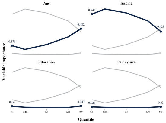
Figure 1. Variable importance across quantiles.

4.2. The Job Training Program

Abadie et al. (2002) use the Job Training Partnership Act (JTPA) data to estimate the quantile treatment effect of job training on the earning distribution2. The data is from Title II of the JTPA in the early 1990’s, which consists of 11,204 samples, 5102 of which are male, and 6102 of which are female. In the estimation, they take 30-month earnings as the outcome variable, enrollment for JTPA service as the treatment variable, and a randomized offer of JTPA enrollment as the instrumental variable. Control variables include education, race, marital status, previous year work status, job training service strategies, age, and whether earnings data is from the second follow-up survey. In the female group, an additional control, aid to families with dependent children (AFDC), is added. We follow the same model specifications when estimating the GRF-IVQR.

Table 3 and Table 4 show that for females, job training program generates a significantly positive treatment effect on earnings at 0.5 and 0.75 quantiles. GRF-IVQR signifies similar results.

Table 3. Effects of JTPA enrollment on earning (male).

	Quantile
	0.15	0.25	0.50	0.75	0.85
AAI	121.000	702.000	1544.000	3131.000	3378.000
	(475.000)	(670.000)	(1073.000)	(1376.000)	(1811.000)
CH	−151.151	528.529	312.312	2697.698	3190.190
	(535.146)	(627.293)	(957.707)	(1547.084)	(1536.335)
GRF-IVQR	−199.114	232.099	1068.086	2630.969	2955.952
	(540.548)	(651.584)	(950.880)	(1571.200)	(1645.931)

Note: GRF-IV: 1814.755 (1022.473). The GRF-IV stands for the 2SLS in the context of generalized random forests. AAI, CH and GRF-IVQR stand for, respectively, Abadie, Angrist and Imbens (2002), Chernozhukov and Hansen (2005) and our estimator. Numbers in parentheses are standard errors.

Table 4. Effects of JTPA enrollment on earning (female).

	Quantile
	0.15	0.25	0.50	0.75	0.85
AAI	324.000	680.000	1742.000	1984.000	1900.000
	(175.000)	(282.000)	(645.000)	(945.000)	(997.000)
CH	35.536	398.398	1566.567	2493.493	1845.345
	(266.445)	(313.555)	(626.065)	(910.474)	(1059.988)
GRF-IVQR	185.141	571.842	1892.934	2431.793	1716.304
	(270.490)	(336.180)	(610.466)	(894.658)	(1119.506)

Note: GRF-IV: 2127.544 (607.943). The GRF-IV stands for the 2SLS in the context of generalized random forests. AAI, CH and GRF-IVQR stand for, respectively, Abadie, Angrist and Imbens (2002), Chernozhukov and Hansen (2005) and our estimator. Numbers in parentheses are standard errors.

For the male group, Table 5 and Figure 2 depicts that work less than 13 weeks (wlkess13) and on-the-job training and/or job search assistance (ojt_jsa) are the most important variables. However, there is no apparent pattern suggesting that variable importance differs across quantiles. The pattern of variable importance resulting from the GRF-IV and the GRF-IVQR are different as well.

Table 5. Variable importance (male).

	GRF-IV	GRF-IVQR at Specific Quantiles
		0.15	0.25	0.50	0.75	0.85
High school or GED	0.11710	0.10009	0.10155	0.08882	0.07741	0.08376
Black	0.04914	0.06883	0.04729	0.09594	0.09909	0.10482
Hispanic	0.05177	0.00000	0.00000	0.00000	0.00000	0.00000
Married	0.12656	0.11679	0.12841	0.09669	0.07070	0.08854
Work less than 13 week in past year	0.09076	0.19681	0.16594	0.19491	0.07749	0.08512
Classroom training	0.05013	0.02939	0.02939	0.03967	0.08669	0.04849
On-the-job training and/or job search assistance	0.08262	0.24453	0.36400	0.27075	0.41578	0.37083
Age from 22 to 25	0.03710	0.04702	0.03930	0.04970	0.03646	0.04310
Age from 26 to 29	0.06769	0.02204	0.02204	0.02498	0.02792	0.06612
Age from 30 to 35	0.04465	0.03233	0.03820	0.04114	0.03673	0.03967
Age from 36 to 44	0.07998	0.02792	0.01910	0.03527	0.03086	0.02351
Age from 45 to 54	0.09737	0.00000	0.00000	0.00000	0.00000	0.00000
Whether data are from second follow-up survey	0.10514	0.11425	0.04476	0.06214	0.04087	0.04604

Note: The GRF-IV stands for the 2SLS in the context of generalized random forests.

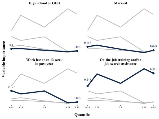
Figure 2. Top 4 variable importance (male).

As to the GRF-IVQR, in Table 5, the variance importance for Hispanics and the age group 45 to 54 are 0 across all quantiles, while the GRF-IV suggests these two variables are of some importance. Possible explanations are as follows. Compared to the GRF-IVQR’s moment condition, the GRF-IV still performs well in nodes with a relatively small amount of data. Consequently, the GRF-IVQR is more restrictive for growing a shallower tree than the GRF-IV. Therefore, some variables used to make a split in deeper nodes will not be chosen by the GRF-IVQR algorithm. Besides, at deeper nodes, the data is very similar in each node. Specifically, this situation occurs frequently with a large number of binary variables, and thus leads to no variation in a certain variable. Therefore, in practical estimation, the GRF-IVQR grows a relatively small tree.

For the female group, Table 6 and Figure 3 depicts that classroom training (class_tr) and on-the-job training and/or job search assistance (ojt_jsa) are the most important variables. The importance of on-the-job training and/or job search assistance decreases across quantiles, which is different from the pattern in the male group. The issue concerning no variation of a binary variable in deeper nodes becomes severe in the female group.

Table 6. Variable importance (female).

	GRF-IV	GRF-IVQR at Specific Quantiles
		0.15	0.25	0.50	0.75	0.85
High school or GED	0.06385	0.02720	0.03360	0.05760	0.04320	0.11040
Black	0.05128	0.03040	0.07200	0.14720	0.12000	0.08800
Hispanic	0.07033	0.00000	0.00000	0.00000	0.00000	0.00000
Married	0.09909	0.03520	0.01120	0.08000	0.06880	0.18240
ADFC	0.14744	0.02658	0.02880	0.08070	0.07881	0.10153
Work less than 13 week in past year	0.05033	0.07717	0.11360	0.08070	0.08301	0.07367
Classroom training	0.15284	0.17735	0.24160	0.34876	0.19237	0.17197
On-the-job training and/or job search assistance	0.06905	0.56049	0.44320	0.16823	0.35140	0.16323
Age from 22 to 25	0.03948	0.00160	0.00480	0.00000	0.00160	0.00000
Age from 26 to 29	0.05355	0.00000	0.00000	0.00000	0.00000	0.00000
Age from 30 to 35	0.05257	0.03040	0.03520	0.01280	0.01600	0.04000
Age from 36 to 44	0.05325	0.00000	0.00000	0.00000	0.00000	0.00000
Age from 45 to 54	0.04129	0.00000	0.00000	0.00000	0.00000	0.00000
Whether data are from second follow-up survey	0.05564	0.03360	0.01600	0.02400	0.04480	0.06880

Note: The GRF-IV stands for the 2SLS in the context of generalized random forests.

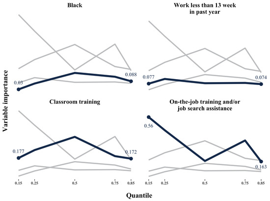
Figure 3. Top 4 variable importance (female).

The variance importance for Hispanics and several age binary variables are 0 across all quantiles, which indicates that in the female group, the aforementioned characteristics variables are more homogeneous over the conditional distribution of earnings.

5. Conclusions

Based on the generalized random forests of Athey et al. (2019), we propose an econometric procedure to estimate the quantile treatment effect. Not only does this method estimate the treatment effect nonparametrically, but our procedure yields a measure of variable importance, in terms of heterogeneity among control variables. We provide the practical algorithm and the associated R codes. We also apply the proposed procedure to reinvestigate the distributional effect of 401(k) participation on net financial assets, and the quantile effect of participating a job training program on earnings. Income, age, education, and family size are identified as the first-four important variables in the 401(k) analysis. In the job training program example, our procedure suggests that the previous year work status and the job training service strategies are important control variables.

Appendix A.1. Improving Efficiency by Doubly Robust Estimators

Chernozhukov et al. (2018) and Athey and Wager (2018) pioneered the use of the doubly robust estimator embedded in a framework of causal machine learning. The resulting estimator becomes more accurate and gains efficiency. In light of their idea, it might be beneficial to incorporate the doubly robust estimation in our methodology.

A doubly robust augmented inverse propensity weighted (AIPW) estimator was introduced by Robins et al. (1994). The AIPW estimator for average treatment effect is constructed by two components as follows.

$$\begin{array}{cc}\hfill {\widehat{\mathrm{ATE}}}_{\mathrm{AIPW}}& =\frac{1}{n}\sum _{i=1}^n\{\left[\frac{D_i{Y}_i}{\widehat{e}\left(X_i\right)}-\frac{(1-D_i)Y_i}{1-\widehat{e}\left(X_i\right)}\right]\hfill \\ \hfill & -\frac{(D_i-\widehat{e}\left(X_i\right))}{\widehat{e}\left(X_i\right)(1-\widehat{e}\left(X_i\right))}\left[(1-\widehat{e}\left(X_i\right))\widehat{\mathbb{E}}\left(Y_i\right|D_i=1,X_i)+\widehat{e}\left(X_i\right)\widehat{\mathbb{E}}\left(Y_i\right|D_i=0,X_i)\right]\},\hfill \end{array}$$

where $e\left(x\right)=P\left[D_i\right|X_i=x]$ being the propensity score. The first line in the equation represents the inverse probability weighted estimator, and the second line depicts a weighted regression. The AIPW estimator is doubly robust because the estimator will be consistent, provided that at least one of the two components is correctly specified.

Appendix A.2. The Doubly Robust Estimation for Causal Forests

Athey and Wager (2019) and their grf R package implement a variant of doubly robust AIPW estimators for causal forests. Specifically, for estimating average treatment effect, their doubly robust estimator is shown as follows.

$$\begin{array}{cc}\hfill \widehat{\mathrm{ATE}}& =\widehat{\gamma }=\frac{1}{n}\sum _{i=1}^n{\widehat{\Gamma }}_i,\hfill \\ \hfill {\widehat{\Gamma }}_i& ={\widehat{\gamma }}^{(-i)}\left(X_i\right)\hfill \\ \hfill & +\frac{D_i-{\widehat{e}}^{(-i)}\left(X_i\right)}{{\widehat{e}}^{(-i)}\left(X_i\right)\left(1-{\widehat{e}}^{(-i)}\left(X_i\right)\right)}\left(Y_i-{\widehat{m}}^{(-i)}\left(X_i\right)-\left(D_i-{\widehat{e}}^{(-i)}\left(X_i\right)\right){\widehat{\gamma }}^{(-i)}\left(X_i\right)\right),\hfill \end{array}$$

where $\widehat{\gamma }\left(X_i\right)$ is the conditional average treatment effect estimator based on causal forest, ${\widehat{\Gamma }}_i$ is the conditional average treatment effect estimator adjusted by inverse probability weighting, $\widehat{m}\left(x\right)$ and $\widehat{e}\left(x\right)$ are the estimators of $E\left[Y\right|X=x]$ and $E\left[D\right|X=x]$ which are based on random forest with honest splitting, and the average treatment effect estimator $\widehat{\gamma }$ is simply the sample average of those adjusted conditional average treatment effect estimates.

Glynn and Quinn (2009) provide some evidence that the doubly robust estimator performs better in terms of efficiency than inverse probability weighting estimators, matching estimators, and regression estimators. To explore how adapting the doubly robust method in the causal forest estimator affects the efficiency and accuracy, we follow their DGP designs and conduct Monte Carlo experiments with different degree of confoundedness. In the simulation, $X_1,X_2$, and $X_3$ are covariates following $N(0,1)$, D is the treatment variable, Y is the outcome variable, and $ϵ$ is the disturbance which follows $N(0,1)$. Two data generating processes are considered. Degree of confoundedness are modeled in three levels: low, moderate, and severe.

Table A1. Simulation setting.

	Outcome (control)		Outcome (treatment)
Simple DGP	$Y=X_2+X_3+ϵ$		$Y=5+3X_2+X_3+ϵ$
Complicate DGP	$Y=X_2+X_3+ϵ$		$Y=5+3X_2+X_3+2X_2^2+2X_3^2+ϵ$
Degree of confoundedness		True treatment assignment probabilities
Low		$P(D=1|X)=\Phi (0.1X_1+0.1X_2+0.05X_1{X}_2)$
Moderate		$P(D=1|X)=\Phi (X_1+X_2+0.5X_1{X}_2)$
Severe		$P(D=1|X)=\Phi (1.5X_1+1.5X_2+0.75X_1{X}_2)$

Table A1. Simulation setting.

	Outcome (control)		Outcome (treatment)
Simple DGP	$Y=X_2+X_3+ϵ$		$Y=5+3X_2+X_3+ϵ$
Complicate DGP	$Y=X_2+X_3+ϵ$		$Y=5+3X_2+X_3+2X_2^2+2X_3^2+ϵ$
Degree of confoundedness		True treatment assignment probabilities
Low		$P(D=1|X)=\Phi (0.1X_1+0.1X_2+0.05X_1{X}_2)$
Moderate		$P(D=1|X)=\Phi (X_1+X_2+0.5X_1{X}_2)$
Severe		$P(D=1|X)=\Phi (1.5X_1+1.5X_2+0.75X_1{X}_2)$

With three different sample sizes, $250,500$, and 1000, three degrees of confoundedness, and two DGP settings, the Monte Carlo results are tabulated in Table A2. The results confirm that the causal forest with doubly robust estimation indeed has efficiency gains over the conventional causal forest.

Table A2. Finite-sample performance: causal forests with doubly robust estimation.

		Linear DGP		Nonlinear DGP
		Causal forest	Causal forest with doubly robust	Causal forest	Causal forest with doubly robust
Sample size	Confoundedness degree	RMSE	RMSE	RMSE	RMSE
250	low	0.3730	0.1693	0.7542	0.3147
250	moderate	0.4200	0.2099	0.9295	0.3914
250	severe	0.4562	0.2218	1.0205	0.3997
500	low	0.3206	0.1081	0.6911	0.1855
500	moderate	0.3634	0.1417	0.8711	0.2320
500	severe	0.4107	0.1497	0.9529	0.2505
1000	low	0.2745	0.0717	0.6041	0.1124
1000	moderate	0.3244	0.1008	0.7755	0.1540
1000	severe	0.3742	0.1098	0.8919	0.1709

Table A2. Finite-sample performance: causal forests with doubly robust estimation.

		Linear DGP		Nonlinear DGP
		Causal forest	Causal forest with doubly robust	Causal forest	Causal forest with doubly robust
Sample size	Confoundedness degree	RMSE	RMSE	RMSE	RMSE
250	low	0.3730	0.1693	0.7542	0.3147
250	moderate	0.4200	0.2099	0.9295	0.3914
250	severe	0.4562	0.2218	1.0205	0.3997
500	low	0.3206	0.1081	0.6911	0.1855
500	moderate	0.3634	0.1417	0.8711	0.2320
500	severe	0.4107	0.1497	0.9529	0.2505
1000	low	0.2745	0.0717	0.6041	0.1124
1000	moderate	0.3244	0.1008	0.7755	0.1540
1000	severe	0.3742	0.1098	0.8919	0.1709

Appendix A.3. The Doubly Robust Estimation for Instrumental Causal Forests

With instrumental variables, Athey and Wager (2018) provide a doubly robust estimator for local average treatment effect; namely

$$\begin{array}{cc}\hfill \widehat{\mathrm{LATE}}& =\widehat{\gamma }=\frac{1}{n}\sum _{i=1}^n{\widehat{\Gamma }}_i,\hfill \\ \hfill {\widehat{\Gamma }}_i& ={\widehat{\gamma }}^{(-i)}\left(X_i\right)\hfill \\ \hfill & +\frac{1}{{\widehat{\Delta }}^{(-i)}\left(X_i\right)}\frac{Z_i-{\widehat{z}}^{(-i)}\left(X_i\right)}{{\widehat{z}}^{(-i)}\left(X_i\right)\left(1-{\widehat{z}}^{(-i)}\left(X_i\right)\right)}\left(Y_i-{\widehat{m}}^{(-i)}\left(X_i\right)-\left(D_i-{\widehat{e}}^{(-i)}\left(X_i\right)\right){\widehat{\gamma }}^{(-i)}\left(X_i\right)\right),\hfill \end{array}$$

where $\widehat{\gamma }\left(X_i\right)$ is the conditional local average treatment effect estimator based on instrumental forest, ${\widehat{\Gamma }}_i$ is the conditional local average treatment effect estimator adjusted by inverse probability weighting, $\widehat{m}\left(x\right)$, $\widehat{e}\left(x\right)$, $\widehat{z}\left(x\right)$, and $\widehat{\Delta }\left(x\right)$ are the estimators of $E\left[Y\right|X=x]$, $E\left[D\right|X=x]$, $E\left[Z\right|X=x]$, and $P\left(D\right|Z=1,X=x)-P(D|Z=0,X=x)$ which are based on random forest with honest splitting, and the local average treatment effect estimator $\widehat{\gamma }$ is simply the sample average of those adjusted conditional local average treatment effect estimates.

Appendix A.4. An Unsolved Task: The Doubly-Robust GRF-IVQR

Researchers would like to incorporate the doubly robust estimation in the GRF-IVQR model, following similar ideas introduced above. However, it remains unclear how to do it. We leave this unsolved task as future work.

Appendix A.5. Identifying Restrictions and Regularity Conditions for the GRF-IVQR

Following Chernozhukov and Hansen (2008), we consider the instrumental variable quantile regression characterizing the structural relationship:

$$\begin{array}{cc}\hfill Y& =D^{\prime }\theta \left(U\right)+X^{\prime }\nu \left(U\right),U|X,Z\sim \mathrm{Uniform}(0,1)\hfill \\ \hfill D& =\delta (X,Z,V)\mathrm{where}V\mathrm{is}\mathrm{statistically}\mathrm{dependent}\mathrm{on}U\hfill \\ \hfill \tau & \mapsto D^{\prime }\theta \left(\tau \right)+X^{\prime }\nu \left(\tau \right)\mathrm{strictly}\mathrm{increasing}\mathrm{in}\tau \hfill \end{array}$$

where

• Y is the scalar outcome variable of interest.
• U is a scalar random variable (rank variable) that aggregates all of the unobserved factors affecting the structural outcome equation.
• D is a vector of endogenous variables determined by $\delta (X,Z,V)$.
• V is a vector of unobserved disturbances determining D and correlated with U.
• Z is a vector of instrumental variables.
• X is a vector of included control variables.

The one-dimensional rank variable and the rank similarity (rank preservation) condition imposed on the outcome equation play an important role in identifying the quantile treatment effect. To derive the standard error of the IVQR estimator, the following assumptions are needed as well.

Assumption CH1.

$Y_i,D_i,X_i,Z_i$ are iid defined on the probability space $\Omega ,F,P$ and have compact support.

Assumption CH2.

For the given τ, $\left(\theta \right(\tau ),\nu (\tau \left)\right)$ is in the interior of the parameter space.

Assumption CH3.

Density $f_Y\left(Y\right|X,D,Z)$ is bounded by a constant $\overline{f}$ a.s.

Assumption CH4.

$\partial E[1(Y<D^{\prime }\theta +X^{\prime }\nu +Z\gamma )\Psi ]/\partial ({\nu }^{\prime },{\gamma }^{\prime })$ at $(\nu ,\gamma )=\left(\nu \right(\theta ,\tau ),\gamma (\theta ,\tau \left)\right)$ has full rank for each θ in Θ, for $\Psi =V_i{(Z_i^{\prime },X_i^{\prime })}^{\prime }$.

Assumption CH5.

$\partial E[1(Y<D^{\prime }\theta +X^{\prime }\nu )\Psi ]/\partial ({\theta }^{\prime },{\nu }^{\prime })$ has full rank at ${(\theta {\left(\tau \right)}^{\prime },\nu {\left(\tau \right)}^{\prime })}^{\prime }$.

Assumption CH6.

The function $(\theta ,\nu )⟼E\left[\{\tau -1(Y<D^{\prime }\theta +X^{\prime }\nu )\Psi \}\right]$ is one-to-one over parameter space.

Assumptions CH1–CH6 are compatible with those imposed in Athey et al. (2019); for example, both sets of assumptions do not apply to time-series data.

Assumption ATW1

(Lipschitz x-signal). For fixed values of $(\theta ,\nu )$, we assume that $M_{\theta ,\nu }\left(x\right):=\mathbb{E}\left[{\psi }_{\theta ,\nu }\left(O\right)\right|X=x]$ is Lipschitz continuous in x.

Assumption ATW2

(Smooth identification). When x is fixed, we assume that the M-function is twice continuously differentiable in $(\theta ,\nu )$ with a uniformly bounded second derivative, and that $V\left(x\right):=V_{\theta \left(x\right),\nu \left(x\right)}\left(x\right)$ is invertible for all $x\in \mathcal{X}$ , with $V_{\theta ,\nu }:=\frac{\partial }{\partial (\theta ,\nu )}{M}_{\theta ,\nu }\left(x\right){|}_{\theta \left(x\right),\nu \left(x\right)}$.

Assumption ATW3

(Lipschitz $(\theta ,\nu )$-variogram). The score functions ${\psi }_{\theta ,\nu }\left(O_i\right)$ have a continuous covariance structure. Writing γ for the worst-case variogram and ${\parallel ·\parallel }_F$ for the Frobenius norm, then for some $L>0$,

$$\begin{array}{cc}\hfill \gamma \left(\left(\begin{array}{c}\theta \\ \nu \end{array}\right),\left(\begin{array}{c}{\theta }^{\prime }\\ {\nu }^{\prime }\end{array}\right)\right)& \le L{∥\left(\begin{array}{c}\theta \\ \nu \end{array}\right)-\left(\begin{array}{c}{\theta }^{\prime }\\ {\nu }^{\prime }\end{array}\right)∥}_2\mathit{for}\mathit{all}(\theta ,\nu ),({\theta }^{\prime },{\nu }^{\prime })\hfill \\ \hfill \gamma \left(\left(\begin{array}{c}\theta \\ \nu \end{array}\right),\left(\begin{array}{c}{\theta }^{\prime }\\ {\nu }^{\prime }\end{array}\right)\right)& :=\underset{x\in \mathcal{X}}{sup}\left\{{∥Var[{\psi }_{\theta ,\nu }\left(O_i\right)-{\psi }_{{\theta }^{\prime },{\nu }^{\prime }}\left(O_i\right)|X_i=x]∥}_F\right\}\hfill \end{array}$$

Assumption ATW4

(Regularity of $\psi$). The ψ-functions can be written as ${\psi }_{\theta ,\nu }\left(O\right)=\lambda (\theta ,\nu ;O_i)+{\zeta }_{\theta ,\nu }\left(g\left(O_i\right)\right)$, such that λ is Lipschitz-continuous in $(\theta ,\nu )$, $g:O_i\to \mathbb{R}$ is a univariate summary of $O_i$, and ${\zeta }_{\theta ,\nu }:\mathbb{R}\to \mathbb{R}$ is any family of monotone and bounded functions.

Assumption ATW5

(Existence of solutions). We assume that, for any weights ${\alpha }_i$ with $\sum {\alpha }_i=1$, the estimating equation $(\widehat{\theta }\left(x\right),\widehat{\nu }\left(x\right))\in {argmin}_{\theta ,\nu }\left\{{∥{\sum }_{i=1}^n{\alpha }_i\left(x\right){\psi }_{\theta ,\nu }\left(O_i\right)∥}_2\right\}$ returns a minimizer $(\widehat{\theta },\widehat{\nu })$ taht at least approximately solves the estimating equation ${∥\sum _{i=1}^n{\alpha }_i{\psi }_{\widehat{\theta },\widehat{\nu }}\left(O_i\right)∥}_2\le Cmax\left\{{\alpha }_i\right\}$, for some constant $C\ge 0$.

Assumption ATW6

(Convexity). The score function ${\psi }_{\theta ,\nu }\left(O_i\right)$ is a negative sub- gradient of a convex function, and the expected score $M_{\theta ,\nu }\left(X_i\right)$ is the negative gradient of a strongly convex function.

Given Assumptions ATW1-ATW6, the Theorems 3 and 5 of Athey et al. (2019) guarantee that the GRF estimator achieves consistency and asymptotic normality. In what follows, we check each assumptions for the proposed GRF-IVQR estimator.

Observe that the score function of the IVQR

$$\begin{array}{c}\hfill {\psi }_{\theta ,\nu }\left(O_i\right)=\left[\tau -1(Y_i\le D_i\theta (\tau ,x)+X_i\nu (\tau ,x))\right]{(Z_i,X_i)}^{\prime }.\end{array}$$

In Chernozhukov and Hansen (2008), the moment functions are conditional on $\{X_i,D_i,Z_i\}$. For simplicity, we write conditional functions as $[·|X_i=x]$ when considering splitting in $X_i$ within the framework of generalized random forests.

Checking Assumption ATW1.

$$\begin{array}{cc}\hfill & \mathbb{E}\left[{\psi }_{\theta (\tau ,x),\nu (\tau ,x)}\left(O_i\right)|X_i=x\right]\hfill \\ \hfill & =\mathbb{E}\left[\left[\tau -1(Y_i\le D_i\theta (\tau ,x)+X_i\nu (\tau ,x))\right]{(Z_i,X_i)}^{\prime }|X_i=x\right]\mathrm{for}\mathrm{all}x\in \mathcal{X}.\hfill \end{array}$$

Thus the expected score function

$$\begin{array}{cc}\hfill M_{\theta ,\nu }\left(x\right)& =\mathbb{E}\left[{\psi }_{\theta ,\nu }\left(O_i\right)|X_i=x\right]\hfill \\ \hfill & =\mathbb{E}\left[\left[\tau -1(Y_i\le D_i\theta +X_i\nu )\right]{(Z_i,X_i)}^{\prime }|X_i=x\right]\hfill \\ \hfill & =\left[\tau -F(Y_i\le D_i\theta +X_i\nu |X_i=x)\right]{(Z_i,x)}^{\prime }.\hfill \end{array}$$

We want the conditional cumulative distribution function is Lipschitz continuous. Since every function with bounded first derivatives is Lipschitz, we need the conditional density is bounded. Assumption CH3 states that the conditional density $f_Y\left(Y\right|X,D,Z)$ is bounded by a constant $\overline{f}$ a.s.. In particular, $f_Y\left(Y\right|X,D,Z)$ is a density of a convolution of a continuous random variable and a discrete random variable, we also need the continuous variable not to be degenerate.

Checking Assumption ATW2.

$$\begin{array}{cc}\hfill M_{\theta ,\nu }\left(x\right)& =\left[\tau -F(D_i\theta +X_i\nu |X_i=x)\right]{(Z_i,x)}^{\prime }.\hfill \\ \hfill V_{\theta ,\nu }\left(x\right)& =\frac{\partial }{\partial (\theta ,\nu )}{M}_{\theta ,\nu }\left(x\right){|}_{\theta (\tau ,x),\nu (\tau ,x)}\hfill \\ \hfill & =\frac{\partial }{\partial (\theta ,\nu )}\left\{\left[\tau -F(D_i\theta +X_i\nu |X_i=x)\right]{(Z_i,x)}^{\prime }\right\}\hfill \\ \hfill & =\left[\begin{array}{cc}-f(D_i\theta +X_i\nu |X_i=x)Z_i^{\prime }{D}_i\hfill & -f(D_i\theta +X_i\nu |X_i=x)x^{\prime }{D}_i\hfill \\ -f(D_i\theta +X_i\nu |X_i=x)Z_i^{\prime }x\hfill & -f(D_i\theta +X_i\nu |X_i=x)x^{\prime }x.\hfill \end{array}\right]\hfill \end{array}$$

We want V is invertible and therefore $\left[\begin{array}{cc}{Z}_i^{\prime }{D}_i\hfill & x^{\prime }{D}_i\hfill \\ Z_i^{\prime }x\hfill & x^{\prime }x\hfill \end{array}\right]$ needs to be invertible. In addition, the conditional density $f(D_i\theta +X_i\nu |X_i=x)$ is required to have continuous uniformly bounded first derivative. If $f(D_i\theta +X_i\nu |X_i=x)$ is continuously differentiable, then its first derivative is uniformly bounded. Those conditions are implied by Assumptions CH4 and CH5. Thus $A_p$ is invertible as well.

Checking Assumption ATW3.

$$\begin{array}{cc}& \gamma \left(\left(\begin{array}{c}\theta \\ \nu \end{array}\right),\left(\begin{array}{c}{\theta }^{\prime }\\ {\nu }^{\prime }\end{array}\right)\right)\hfill \\ \hfill =& \underset{x\in \mathcal{X}}{sup}\left\{{∥Var[{\psi }_{\theta ,\nu }\left(O_i\right)-{\psi }_{{\theta }^{\prime },{\nu }^{\prime }}\left(O_i\right)|X_i=x]∥}_F\right\}\hfill \\ \hfill =& \underset{x\in \mathcal{X}}{sup}\{\left.∥Var{\left[\left[\tau -1(Y_i\le D_i\theta +X_i\nu )\right]{(Z_i,X_i)}^{\prime }-\left[\tau -1(Y_i\le D_i{\theta }^{\prime }+X_i{\nu }^{\prime })\right]{(Z_i,X_i)}^{\prime }\left|X_i=x\right]\right.∥}_F\right\}\hfill \\ \hfill =& \underset{x\in \mathcal{X}}{sup}\left\{{∥{(Z_i,x)}^{\prime }(Z_i,x)Var\left[-1(Y_i\le D_i\theta +X_i\nu )+1(Y_i\le D_i{\theta }^{\prime }+X_i{\nu }^{\prime })\right]\left|X_i=x\right]∥}_F\right\}\hfill \\ \hfill =& \underset{x\in \mathcal{X}}{sup}\{\parallel {(Z_i,x)}^{\prime }(Z_i,x)\left[F(D_i\theta +X_i\nu |X_i=x)-F(D_i{\theta }^{\prime }+X_i{\nu }^{\prime }|X_i=x)\right]\hfill \\ & \left[1-\left[F(D_i\theta +X_i\nu |X_i=x)-F(D_i{\theta }^{\prime }+X_i{\nu }^{\prime }|X_i=x)\right]\right]{\parallel }_F\}.\hfill \end{array}$$

Taylor expansion implies the following approximation of $\gamma$.

$$\begin{array}{c}\hfill \gamma \left(\left(\begin{array}{c}\theta \\ \nu \end{array}\right),\left(\begin{array}{c}{\theta }^{\prime }\\ {\nu }^{\prime }\end{array}\right)\right)\approx \underset{x\in \mathcal{X}}{sup}\left\{{∥{(Z_i,x)}^{\prime }(Z_i,x)\left[f\left(y\right|X_i=x)\left(D_i(\theta -{\theta }^{\prime })+X_i(\nu -{\nu }^{\prime })\right)\right]∥}_F\right\}.\end{array}$$

Since the conditional probability density function is bounded, there exists a $L>0$, such that

$$\begin{array}{c}\hfill \gamma \left(\left(\begin{array}{c}\theta \\ \nu \end{array}\right),\left(\begin{array}{c}{\theta }^{\prime }\\ {\nu }^{\prime }\end{array}\right)\right)\le L{∥\left(\begin{array}{c}\theta \\ \nu \end{array}\right)-\left(\begin{array}{c}{\theta }^{\prime }\\ {\nu }^{\prime }\end{array}\right)∥}_2.\end{array}$$

Checking Assumption ATW4. The score function can be written as

$$\begin{array}{cc}\hfill {\psi }_{\theta ,\nu }\left(O_i\right)& =\left[\tau -1(Y_i\le D_i\theta +X_i\nu )\right]{(Z_i,X_i)}^{\prime }\hfill \\ \hfill & =\lambda (\theta ,\nu ;O_i)+{\zeta }_{\theta ,\nu }\left(g\left(O_i\right)\right),\hfill \end{array}$$

where

$$\begin{array}{cc}\hfill g\left(O_i\right)& =Y_i,\mathrm{and}\hfill \\ \hfill {\zeta }_{\theta ,\nu }\left(g\left(O_i\right)\right)& =\left(\begin{array}{c}\left[\tau -1(Y_i\le D_i\theta +X_i\nu )\right]Z_i\\ \\ \left[\tau -1(Y_i\le D_i\theta +X_i\nu )\right]X_i\end{array}\right).\hfill \end{array}$$

Checking Assumption ATW5. Since Assumption ATW5 is used to ensure the existence of solutions, it is required.

Checking Assumption ATW6. With a V-shaped check function of the instrumental variable quantile regression, the corresponding score function ${\psi }_{\theta ,\nu }\left(O_i\right)$ is a negative subgradient of a convex function, and the expected score function $M_{\theta ,\nu }\left(x\right)$ is a negative gradient of a strongly convex function. Therefore, Assumption ATW6 holds.

Corollary.(Consistency and asymptotic normality of the GRF-IVQR estimator) Given Assumptions ATW1-6, Assumptions CH1-6, and Theorems 3 and 5 of Athey et al. (2019), the GRF-IVQR is consistent and asymptotically normal:

$$\begin{array}{c}\hfill \frac{{\widehat{\theta }}_n\left(x\right)-\theta \left(x\right)}{{\sigma }_n\left(x\right)}\to N(0,1).\end{array}$$

The variance estimator

$$\begin{array}{c}\hfill {\widehat{\sigma }}_n^2={\xi }^{\top }{\widehat{V}}_n{\left(x\right)}^{-1}{\widehat{H}}_n\left(x\right){\left({\widehat{V}}_n{\left(x\right)}^{-1}\right)}^{\top }\xi ,\end{array}$$

where ${\widehat{V}}_n\left(x\right)$ and ${\widehat{H}}_n\left(x\right)$ are consistent estimators for the $V_{\theta ,\nu }\left(x\right)$ and $H_n\left(x\right)=Var{\sum }_{i=1}^n{\alpha }_i{\psi }_{\theta ,\nu }\left(O_i\right)$ respectively.

References

- Abadie, Alberto, Joshua Angrist, and Guido Imbens. 2002. Instrumental variables estimates of the effect of subsidized training on the quantiles of trainee earnings. Econometrica 70: 91–117. [Google Scholar] [CrossRef]
- Athey, Susan, and Guido Imbens. 2016. Recursive partitioning for heterogeneous causal effects. Proceedings of the National Academy of Sciences 113: 7353–60. [Google Scholar] [CrossRef] [PubMed]
- Athey, Susan, and Guido Imbens. 2019. Machine learning method that economists should know about. Annual Review of Economics 11: 685–725. [Google Scholar] [CrossRef]
- Athey, Susan, Julie Tibshirani, and Stefan Wager. 2019. Generalized random forests. The Annals of Statistics 47: 1148–78. [Google Scholar] [CrossRef]
- Athey, Susan, and Stefan Wager. 2018. Efficient policy learning. arXiv arXiv:1702.02896v4. [Google Scholar]
- Athey, Susan, and Stefan Wager. 2019. Estimating treatment effects with causal forests: An application. arXiv arXiv:1902.07409. [Google Scholar]
- Breiman, Leo. 2001. Random forests. Machine Learning 45: 5–32. [Google Scholar] [CrossRef]
- Chen, Jau-er, and Jia-Jyun Tien. 2019. Debiased/Double Machine Learning for Instrumental Variable Quantile Regressions. Working Paper. Taipei, Taiwan: Center for Research in Econometric Theory and Applications, National Taiwan University. [Google Scholar]
- Chernozhukov, Victor, Denis Chetverikov, Mert Demirer, Esther Duflo, Christian Hansen, Whitney Newey, and James Robins. 2018. Double/debiased machine learning for treatment and structural parameters. The Econometrics Journal 21: C1–C68. [Google Scholar] [CrossRef]
- Chernozhukov, Victor, and Christian Hansen. 2004. The effects of 401(k) participation on the wealth distribution: An Instrumental quantile regression analysis. Review of Economics and Statistics 86: 735–51. [Google Scholar] [CrossRef]
- Chernozhukov, Victor, and Christian Hansen. 2005. An IV model of quantile treatment effects. Econometrica 73: 245–61. [Google Scholar] [CrossRef]
- Chernozhukov, Victor, and Christian Hansen. 2008. Instrumental variable quantile regression: A robust inference approach. Journal of Econometrics 142: 379–98. [Google Scholar] [CrossRef]
- Chernozhukov, Victor, and Christian Hansen. 2013. NBER 2013 Summer Institute: Econometric Methods for High-Dimensional Data. Available online: http://www.nber.org/econometrics_minicourse_2013/ (accessed on 15 July 2013).
- Chiou, Yan-Yu, Mei-Yuan Chen, and Jau-er Chen. 2018. Nonparametric regression with multiple thresholds: Estimation and inference. Journal of Econometrics 206: 472–514. [Google Scholar] [CrossRef]
- Davis, Jonathan M. V., and Sara B. Heller. 2017. Using causal forests to predict treatment heterogeneity: An application to summer jobs. American Economic Review 107: 546–50. [Google Scholar] [CrossRef]
- Frandsen, Brigham R., and Lars J. Lefgren. 2018. Testing rank similarity. Review of Economics and Statistics 100: 86–91. [Google Scholar] [CrossRef]
- Gilchrist, Duncan Sheppard, and Emily Glassberg Sands. 2016. Something to talk about: Social spillovers in movie consumption. Journal of Political Economy 124: 1339–82. [Google Scholar] [CrossRef]
- Glynn, Adam N., and Kevin M. Quinn. 2009. An introduction to the augmented inverse propensity weighted estimator. Political Analysis 18: 36–56. [Google Scholar] [CrossRef]
- Guilhem, Bascle, Louis Mulotte, and Jau-er Chen. 2019. Addressing Strategy endogeneity and performance heterogeneity: Evidence from firm multinationality. Academy of Management Proceedings 2019: 12733. [Google Scholar]
- O’Neill, Eoghan, and Melvyn Weeks. 2018. Causal tree estimation of heterogeneous household response to time-of-use electricity pricing schemes. arXiv arXiv:1810.09179. [Google Scholar]
- Robins, James M., Andrea Rotnitzky, and Lue Ping Zhao. 1994. Estimation of regression coefficients when some regressors are not always observed. Journal of the American Statistical Association 89: 846–66. [Google Scholar] [CrossRef]
- Strittmatter, Anthony. 2019. Heterogeneous earnings effects of the job corps by gender: A translated quantile apporach. Labour Economics 61: 101760. [Google Scholar] [CrossRef]
- Wager, Stephan, and Susan Athey. 2018. Estimation and inference of heterogeneous treatment effects using random forests. Journal of the American Statistical Association 113: 1228–42. [Google Scholar] [CrossRef]