Construction and Applications of a Composite Model Based on Skew-Normal and Skew-t Distributions

Abstract

Financial return distributions often exhibit central asymmetry and heavy-tailed extremes, challenging standard parametric models. We propose a novel composite distribution integrating a skew-normal center with skew-t tails, partitioning the support into three regions with smooth junctions. The skew-normal component captures moderate central asymmetry, while the skew-t tails model extreme events with power-law decay, with tail weights determined by continuity constraints and thresholds selected via Hill plots. Monte Carlo simulations show that the composite model achieves superior global fit, lower-tail KS statistics, and stable parameter estimation compared with skew-normal and skew-t benchmarks. We further conduct simulation-based and empirical backtesting of risk measures, including Value-at-Risk (VaR) and Expected Shortfall (ES), using generated datasets and 2083 TSLA daily log returns (2017–2025), demonstrating accurate tail risk capture and reliable risk forecasts. Empirical fitting also yields improved log-likelihood and diagnostic measures (P–P, Q–Q, and negative log P–P plots). Overall, the proposed composite distribution provides a flexible theoretically grounded framework for modeling asymmetric and heavy-tailed financial returns, with practical advantages in risk assessment, extreme event analysis, and financial risk management.

1. Introduction

The composite distribution theory proposed by Cooray and Ananda (2005) represents a significant development in statistical distribution theory in recent years. Due to its conceptual simplicity and structural flexibility, it has garnered considerable attention from the theoretical community. Over the past decade, the theory has been continuously refined and extended, leading to the emergence of various forms of composite distributions. However, in terms of practical applications, this distribution theory has primarily been used to model insurance claim data in the insurance industry. Only recently has it begun to be explored in areas such as urban size distributions, with little application observed beyond these domains (C. Wang, 2018).

Cooray and Ananda (2005) noted that insurance claim data often exhibit two key features: severe right skewness and frequent occurrences of high-claim values. Previous studies typically used single distributions, such as lognormal or (generalized) Pareto distributions for modeling. However, this approach presents certain issues. For instance, the lognormal distribution tends to underestimate large claims, while the Pareto distribution underestimates small claims. To effectively capture both small and large claims within a single distribution, one viable approach is to use a composite distribution. In this model, the lognormal distribution is applied to the lower range of claim values, while the Pareto distribution is used for the higher range. Cooray and Ananda (2005) thus proposed the lognormal–Pareto composite model, where the point separating the two distributions is referred to as the threshold value. Claims below this threshold are assumed to follow a lognormal distribution, while those above follow a Pareto distribution. They successfully applied this model to Danish fire loss data.

Subsequently, Preda and Ciumara (2006) and Cooray (2009) extended the approach, and Scollnik (2007), as well as Nadarajah and Bakar (2014), developed composite distribution models with variable weights and continuity, which have been widely used in practical research. M.-G. Wang and Meng (2014, 2017) constructed three types of composite distributions using different combinations of distributions to fit insurance loss and catastrophe loss data. Chen and Wang (2024) developed a folded Gamma distribution with strong peakedness and heavy-tail properties by constructing a compound model based on the Gamma distribution. Guo and Zhang (2021) introduced a Mixed Erlang–Pareto compound distribution as an alternative modeling approach for catastrophe loss risk evaluation.

Essentially, composite distribution theory involves two key components: the selection of the two distributions applied before and after the threshold point and the allocation of proportions between these two distributions, commonly referred to as mixing weights. Based on whether these mixing weights are fixed or variable, composite distributions can be classified into two categories: those with fixed mixing weights and those with variable mixing weights.

The composite distribution theory proposed by Cooray and Ananda (2005) represents a significant development in statistical distribution theory in recent years. Due to its conceptual simplicity and structural flexibility, it has garnered considerable attention from the theoretical community. Over the past decade, the theory has been continuously refined and extended, leading to the emergence of various forms of composite distributions. In practical applications, however, this distribution theory has primarily been used to model insurance claim data in the insurance industry, with only recent exploration in areas such as urban size distributions (C. Wang, 2018). Cooray and Ananda (2005) noted that insurance claim data often exhibit two key features: severe right skewness and frequent occurrences of high-claim values. Previous studies typically used single distributions, such as lognormal or (generalized) Pareto distributions, but these approaches either underestimate large claims or fail to capture small claims adequately. To address these limitations, the lognormal–Pareto composite model was proposed, where a threshold separates the lower and upper ranges of claims, modeled by lognormal and Pareto distributions, respectively. Subsequent studies extended the approach (Chen & Wang, 2024; Cooray, 2009; Guo & Zhang, 2021; Nadarajah & Bakar, 2014; Preda & Ciumara, 2006; Scollnik, 2007; M.-G. Wang & Meng, 2014, 2017), introducing variable weights, continuity constraints, and alternative combinations of distributions to fit insurance loss and catastrophe data. Essentially, composite distribution theory involves two key components: the selection of the two distributions applied before and after the threshold and the allocation of proportions between them, commonly referred to as mixing weights. Based on whether these weights are fixed or variable, composite distributions can be classified into two categories.

Although composite distribution theory has achieved significant success in modeling non-negative, right-skewed, and heavy-tailed data such as insurance claims and catastrophic losses, most existing studies focus on distributions defined over the positive real line and primarily emphasize right-tail behavior. In many practical applications, including finance, macroeconomics, and environmental science, data are often distributed over the entire real line and may exhibit complex asymmetries, ranging from right-skewness and left-skewness to symmetry. This observation highlights the limitations of conventional composite distribution models when dealing with broader and more diverse data structures.

It is important to note that, while numerous composite distributions have been developed for non-negative, right-skewed, and heavy-tailed data, these models are fundamentally restricted to the positive real line $[0,+\infty )$. In contrast, the composite distribution proposed in this study is specifically designed for real-valued data over the entire real line $(-\infty ,+\infty )$, which is typical for financial return series and many macroeconomic indicators. Therefore, a direct empirical comparison with existing composite distributions is not feasible or meaningful as those models cannot accommodate negative observations that frequently occur in such data. This distinction highlights the novelty of our approach, which simultaneously captures central asymmetry and heavy-tailed behavior on both sides of the distribution, features that conventional composite distributions do not address.

Motivated by these considerations, the present study proposes a novel composite model that combines the skew-normal and skew-t distributions. The skew-normal distribution is effective in modeling light-tailed skewness in the central part of the data, while the skew-t distribution accommodates heavy-tailed and pronounced skewed behavior in the extremes. This composite structure enhances modeling flexibility, improves the ability to capture extreme values and complex skewed patterns, and provides a unified framework for representing real-world financial and macroeconomic data distributions.

Skew-normal and skew-t distributions are two commonly used asymmetric distributions. This study is based on the skew-normal and skew-t distributions developed by Azzalini (2013). The former is effective in modeling skewed data with light tails, while the latter is capable of handling both skewness and heavy-tailed behavior (Azzalini, 1985; Azzalini & Capitanio, 2003). In practical applications, it is often observed that data may exhibit light-tailed but skewed characteristics in the lower range and heavier tails with stronger skewness in the upper range (Eling, 2012). In such cases, a single distribution may struggle to adequately capture the differing distributional patterns across the entire data range.

As a result, constructing a composite distribution model based on skew-normal and skew-t distributions becomes a natural and reasonable approach. Specifically, a skew-normal distribution can be applied to the lower part of the data to capture light-tailed skewness, while a skew-t distribution can be used for the upper part to model heavy-tailed and more pronounced skewed behavior. This composite structure not only enhances modeling flexibility but also improves the ability to capture extreme values and complex skewed patterns, making it more suitable for representing real-world data distributions.

Despite ongoing advancements and extensions in the study of composite distributions, the difficulty in determining appropriate thresholds continues to hinder the construction of certain models. Nonetheless, several researchers have tackled this issue and proposed a variety of solutions, including Lang et al. (1999), Dupuis (1999), Zoglat et al. (2014), and Thompson et al. (2009). Their approaches range from graphical methods based on visual inspection to analytical techniques involving goodness-of-fit tests, as well as hybrid strategies that integrate both approaches (Chukwudum et al., 2020).

The Hill estimator was first proposed by Bruce M. Hill in his seminal 1975 paper (Hill, 1975). It is designed to provide an effective estimation of the tail index for random variables with heavy-tailed characteristics. The method is rooted in extreme value theory and based on the assumption that the extreme portion of the data follows a Pareto-type power-law (Clauset et al., 2009) distribution. The Hill estimator calculates the tail index by using the logarithmic spacing between the largest observations, thereby capturing the decay rate of the tail. Due to its simplicity, computational efficiency, and favorable asymptotic properties in modeling power-law tails, the Hill method has become a widely used tool in fields such as financial risk management, network science, and actuarial science, particularly for analyzing extreme events, such as market crashes, catastrophic insurance claims, or natural disasters (Luckstead & Devadoss, 2017; Scarrott & MacDonald, 2012). Notably, the Hill plot has proven useful for determining whether a distribution exhibits power-law behavior and for identifying the threshold at which the power-law tail begins, providing both visual and quantitative guidance in empirical tail modeling. This study applies the Hill estimator to real-world data to analyze its effectiveness in tail identification and parameter estimation, serving as a foundation for subsequent threshold-based distribution fitting.

The remainder of this manuscript is organized as follows. Section 2 introduces the construction of the proposed composite distribution and its tail properties. Section 3 validates the model using Monte Carlo simulations, including sensitivity analysis. Section 4 applies the proposed distribution to empirical data for parameter estimation and model fitting. Section 5 presents simulation-based and empirical backtesting of risk measures, including Value-at-Risk (VaR) and Expected Shortfall (ES), using both generated datasets and TSLA daily log returns. Finally, Section 6 concludes the study and discusses potential directions for future research.

2. Construction of Composite Distributions and Tail Analysis

2.1. Composite Distribution

Financial returns and other empirical data often exhibit asymmetry(skewness) in the central region and heavy tails (extreme events) in the margins. A single standard distribution, such as the skew-normal or skew-t distribution, may capture either the central shape or the tail behavior well but rarely both simultaneously. To address this limitation, we propose a composite distribution that blends a skew-normal core with skew-t tails, thereby combining the strengths of both families in a piecewise-continuous framework capable of modeling central asymmetry and heavy-tailed extremes.

The theoretical motivation for combining skew-normal and skew-t distributions arises from the distinct economic and statistical mechanisms governing ordinary market fluctuations versus extreme events. In the central region of return distributions, asymmetry typically originates from liquidity imbalances, heterogeneous trading strategies, and market microstructure frictions. The skew-normal distribution provides an analytically tractable and flexible structure to model such moderate asymmetric variations while maintaining light tails. However, it is inadequate for capturing the heavy-tailed patterns associated with large market movements.

Conversely, the skew-t distribution offers a principled framework for modeling power-law decay, volatility bursts, and asymmetric tail behavior driven by rare but impactful economic shocks. Yet, its inherently heavy-tailed nature forces the entire density—including the center—to inherit tail-driven properties, reducing interpretability and deteriorating the fit when central asymmetry is mild. By integrating a skew-normal center with skew-t tails through a smooth double-junction structure, the proposed composite distribution achieves a coherent decomposition between regular return dynamics and extreme event behavior. This hybrid structure enables the simultaneous modeling of central asymmetry and tail risk, providing a theoretically grounded and empirically effective representation of financial return distributions.

Let $\varphi (·)$ and $\mathsf{\Phi }(·)$ denote the standard normal probability density function (PDF) and cumulative distribution function (CDF), respectively. Let $t_{\nu }(·)$ and $T_{\nu }(·)$ denote the PDF and CDF of the standard Student-t distribution with $\nu$ degrees of freedom.

The skew-normal PDF is defined as

$$s_n(x;\xi ,\omega ,\alpha )={\displaystyle \frac{2}{\omega }}\varphi \left({\displaystyle \frac{x-\xi }{\omega }}\right)\mathsf{\Phi }\left(\alpha {\displaystyle \frac{x-\xi }{\omega }}\right),$$

(1)

where $\xi$ and $\omega >0$ are the location and scale parameters, and $\alpha$ controls skewness. For brevity, we write $s_n\left(x\right)$ and denote its CDF by $S_n\left(x\right)$.

Similarly, the skew-t PDF is given by

$$s_t(x;{\xi }_t,{\omega }_t,{\alpha }_t,\nu )={\displaystyle \frac{2}{{\omega }_t}}{t}_{\nu }\left({\displaystyle \frac{x-{\xi }_t}{{\omega }_t}}\right)T_{\nu +1}\left({\alpha }_t{\displaystyle \frac{x-{\xi }_t}{{\omega }_t}}\sqrt{{\displaystyle \frac{\nu +1}{\nu +{\left(\frac{x-{\xi }_t}{{\omega }_t}\right)}^2}}}\right),$$

(2)

where $t_{\nu }(·)$ and $T_{\nu +1}(·)$ are the standard Student-t PDF and CDF with $\nu$ and $\nu +1$ degrees of freedom, respectively. For brevity, we write $s_t\left(x\right)$ and denote its CDF by $S_t\left(x\right)$.

We partition the support of the random variable into three regions:

$$(-\infty ,{\theta }_1],({\theta }_1,{\theta }_2),[{\theta }_2,\infty ),$$

where ${\theta }_1$ and ${\theta }_2$ are threshold parameters defining the junctions between the tails and the central region.

The PDF of the composite distribution is defined as

$$f_{\mathrm{composite}}\left(x\right)=\left\{\begin{array}{cc}{r}_1{\displaystyle \frac{s_t\left(x\right)}{S_t\left({\theta }_1\right)}},\hfill & x\le {\theta }_1,\hfill \\ (1-r_1-r_2){\displaystyle \frac{s_n\left(x\right)}{S_n\left({\theta }_2\right)-S_n\left({\theta }_1\right)}},\hfill & {\theta }_1<x<{\theta }_2,\hfill \\ r_2{\displaystyle \frac{s_t\left(x\right)}{1-S_t\left({\theta }_2\right)}},\hfill & x\ge {\theta }_2,\hfill \end{array}\right.$$

(3)

where $r_1,r_2$ are tail weights satisfying $0\le r_1,r_2\le 1$, and the central weight $1-r_1-r_2$ must be non-negative to ensure a valid density. $s_n\left(x\right)$ and $S_n\left(x\right)$ denote the skew-normal PDF and CDF, respectively (see Equation (1)), and $s_t\left(x\right)$ and $S_t\left(x\right)$ denote the skew-t PDF and CDF, respectively (see Equation (2)).

The composite distribution is fully characterized by the following parameters: ${\theta }_1,{\theta }_2$ (junction thresholds), $r_1,r_2$ (tail weights determined by the continuity conditions), ${\xi }_c,{\omega }_c,{\alpha }_c$ (location, scale, and skewness of the central skew-normal component), and ${\xi }_{tc},{\omega }_{tc},{\alpha }_{tc},{\nu }_c$ (location, scale, skewness, and degrees of freedom of the skew-t component used for both tails).

Continuity at the junctions is imposed by requiring

$$f\left({\theta }_1^{-}\right)=f\left({\theta }_1^{+}\right),f\left({\theta }_2^{-}\right)=f\left({\theta }_2^{+}\right).$$

Solving these equations yields the tail weights $r_1$ and $r_2$:

$$\begin{array}{cc}\hfill r_1& ={\displaystyle \frac{s_t\left({\theta }_2\right)s_n\left({\theta }_1\right)S_t\left({\theta }_1\right)}{s_t\left({\theta }_1\right)s_t\left({\theta }_2\right)[S_n\left({\theta }_2\right)-S_n\left({\theta }_1\right)]+s_t\left({\theta }_2\right)s_n\left({\theta }_1\right)S_t\left({\theta }_1\right)+s_t\left({\theta }_1\right)s_n\left({\theta }_2\right)[1-S_t\left({\theta }_2\right)]}},\hfill \\ \hfill r_2& =1-r_1{\displaystyle \frac{s_t\left({\theta }_1\right)[S_n\left({\theta }_2\right)-S_n\left({\theta }_1\right)]+S_t\left({\theta }_1\right)s_n\left({\theta }_1\right)}{S_t\left({\theta }_1\right)s_n\left({\theta }_1\right)}}.\hfill \end{array}$$

(4)

The CDF of the composite distribution follows as

$$F_{\mathrm{composite}}\left(x\right)=\left\{\begin{array}{cc}{\displaystyle r_1\frac{1}{S_t\left({\theta }_1\right)}{\int }_{-\infty }^x{s}_t\left(z\right)dz,}\hfill & x\le {\theta }_1,\hfill \\ {\displaystyle r_1+(1-r_1-r_2)\frac{1}{S_n\left({\theta }_2\right)-S_n\left({\theta }_1\right)}{\int }_{{\theta }_1}^x{s}_n\left(z\right)dz,}\hfill & {\theta }_1<x<{\theta }_2,\hfill \\ {\displaystyle (1-r_2)+r_2\frac{1}{1-S_t\left({\theta }_2\right)}{\int }_{{\theta }_2}^x{s}_t\left(z\right)dz,}\hfill & x\ge {\theta }_2,\hfill \end{array}\right.$$

(5)

which ensures that $F_{\mathrm{composite}}\left(x\right)$ is continuous and monotonically increasing over $\mathbb{R}$.

In Equations (3)–(5), the shorthand $s_n\left(x\right)$ and $s_t\left(x\right)$ represent the PDFs with the composite parameters:

$$s_n\left(x\right)\equiv s_n(x;{\xi }_c,{\omega }_c,{\alpha }_c),s_t\left(x\right)\equiv s_t(x;{\xi }_{tc},{\omega }_{tc},{\alpha }_{tc},{\nu }_c),$$

where $s_n\left(x\right)$ is applied to the central region and $s_t\left(x\right)$ to both tails. This notation clearly distinguishes the parameters of the composite distribution from those of the standalone skew-normal and skew-t distributions fitted in the empirical analysis.

The full set of composite distribution parameters is given by

$${\mathsf{\Theta }}_{\mathrm{composite}}=\left({\theta }_1,{\theta }_2,r_1,r_2,{\xi }_c,{\omega }_c,{\alpha }_c,{\xi }_{tc},{\omega }_{tc},{\alpha }_{tc},{\nu }_c\right),$$

where ${\theta }_1,{\theta }_2$ are the connection thresholds, $r_1,r_2$ the tail weights, ${\xi }_c,{\omega }_c,{\alpha }_c$ the parameters of the central skew-normal distribution, and ${\xi }_{tc},{\omega }_{tc},{\alpha }_{tc},{\nu }_c$ the parameters of the left and right skew-t tails.

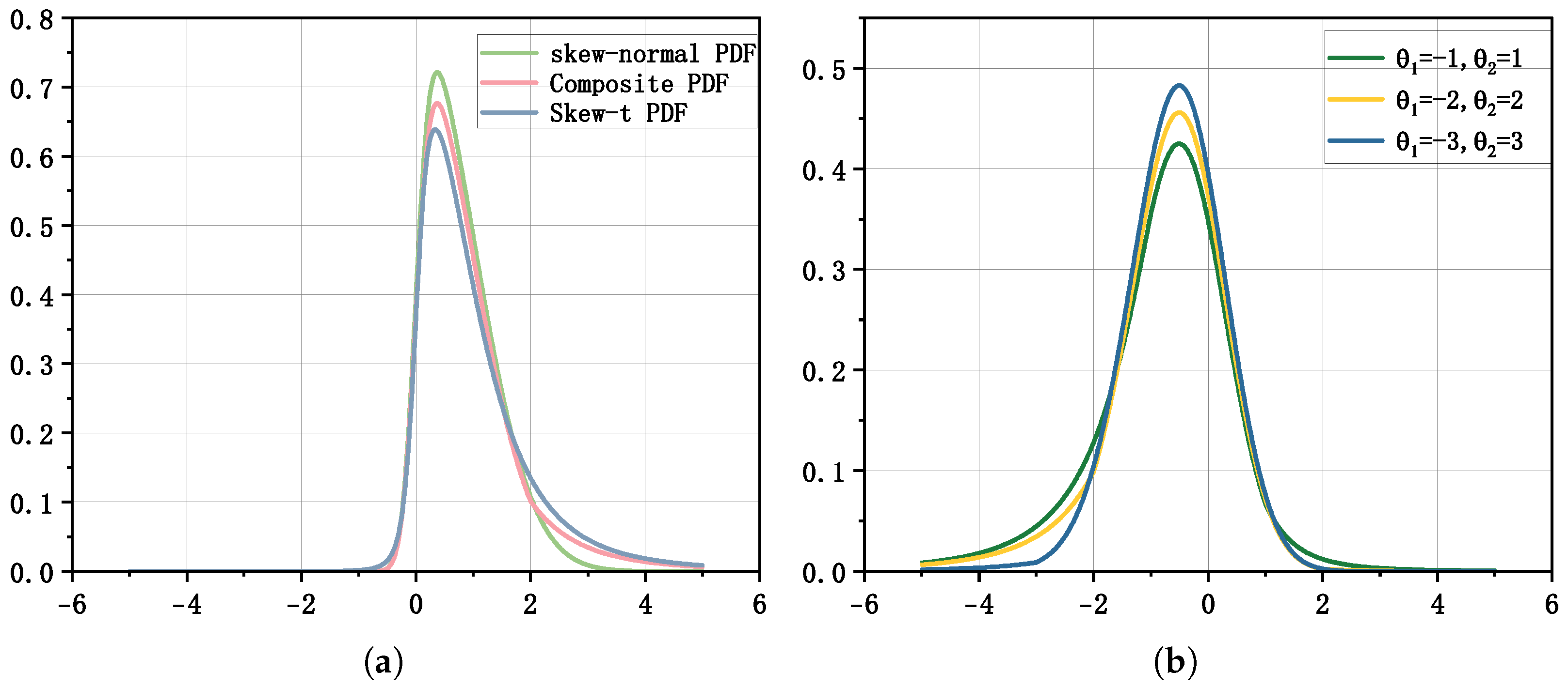
Figure 1 compares the proposed composite distribution with its single-component counterparts. The right panel illustrates how the composite PDF responds to different threshold settings $({\theta }_1,{\theta }_2)$. As the thresholds move further apart, the tail weights $r_1$ and $r_2$ decrease, emphasizing the central region, whereas smaller thresholds increase the contribution of the tails.

Figure 1. Comparison between the composite distribution and single distributions, and composite distribution curves under several threshold settings. (a) Skew-normal, skew-t, and composite distribution density curves. (b) Composite distribution density curves for ${\theta }_1=(-1,-2,-3)$ and ${\theta }_2=(1,2,3)$.

2.2. Power-Law Tail of the Skew-t Distribution and Threshold Selection via the Hill Estimator

Extreme events in financial returns, such as market crashes or surges, are often determined by the behavior of the distribution tails. Extreme value theory (EVT) provides a rigorous framework to analyze such tails, and the Hill estimator (Hill, 1975) is a standard tool to estimate the tail index, which quantifies tail heaviness. Accurate estimation of the tail index is crucial for risk management, Value-at-Risk (VaR) calculations, and other measures sensitive to extreme outcomes.

To apply EVT and the Hill estimator to our composite model, it is important to understand the asymptotic behavior of the tails of the skew-t distribution used for modeling both left and right extremes. In particular, we need to establish that the skew-t distribution exhibits power-law decay, identify the tail exponent, and understand how skewness affects the relative weights of the left and right tails.

2.2.1. Power-Law Behavior in the Tails

We analyze the asymptotic behavior of the skew-t PDF defined in Equation (2). For convenience, define the standardized variable

$$y={\displaystyle \frac{x-{\xi }_t}{{\omega }_t}}.$$

As $\left|y\right|\to \infty$, the PDF exhibits power-law decay. In terms of the original variable x, this is

$$s_t\left(x\right)\sim \left\{\begin{array}{cc}{C}_{+}{(x-{\xi }_t)}^{-(\nu +1)},\hfill & x\to +\infty ,\hfill \\ C_{-}{|x-{\xi }_t|}^{-(\nu +1)},\hfill & x\to -\infty ,\hfill \end{array}\right.$$

where $C_{+}$ and $C_{-}$ are positive constants that generally differ when ${\alpha }_t\ne 0$, reflecting the skewness of the distribution. The tail exponent $\nu +1$ depends solely on the degrees of freedom $\nu$. Mathematically, a power-law tail is defined by $\mathbb{P}(X>x)\sim L\left(x\right)x^{-\kappa }$ for some slowly varying function $L\left(x\right)$ and tail exponent $\kappa >0$; here, $L\left(x\right)$ is asymptotically constant, so the skew-t exhibits a pure power-law tail with $\kappa =\nu +1$.

Although the constants $C_{+}$ and $C_{-}$ differ due to skewness, the tail exponent $\nu +1$ is the same for both tails. This ensures that the Hill estimator consistently estimates the tail index independent of skewness. Furthermore, the asymptotic power-law behavior validates the use of EVT as extreme quantiles are primarily determined by tail decay rather than the shape of the central distribution.

2.2.2. Interpretation and Implications

Several key points follow from this analysis:

• The tail exponent $\nu +1$ determines the rate at which extreme probabilities decay. Smaller $\nu$ corresponds to heavier tails, implying a higher likelihood of extreme returns.
• The constants $C_{+}$ and $C_{-}$ reflect the relative magnitude of the tails and capture skewness: even with identical tail exponents, one tail may be substantially heavier than the other.
• Knowledge of the tail behavior justifies applying the Hill estimator to empirical data to estimate $\nu$. Since the estimator relies on asymptotic power-law behavior, the skew-t tail ensures the correct tail index is targeted.
• In practical applications such as VaR or stress testing, both the tail exponent and the skewness constants are relevant: $\nu +1$ determines how quickly extreme risk decays, while the ratio $C_{+}/C_{-}$ indicates whether positive or negative extremes are more likely.
• When applying the Hill estimator, a threshold k must be chosen to balance bias and variance. Understanding the skew-t tail can guide this selection, for example by focusing on the heavier tail or using symmetric thresholds to capture both extremes.
• We note that, while the skew-t distribution provides a flexible parametric framework for modeling heavy tails, empirical financial data do not always strictly follow classical power-law decay, especially during regime shifts, market anomalies, or structural breaks. Therefore, the skew-t tail assumption serves as an approximation rather than a universal description for all assets or market conditions.

In summary, the skew-t distribution in Equation (2) exhibits power-law decay in both tails, with tail exponent $\nu +1$ and skewness-dependent constants $C_{\pm }$. This provides a theoretical foundation for EVT-based tail analysis and supports the use of the Hill estimator for threshold selection in extreme value modeling.

2.2.3. Hill Estimator for Tail Index and Threshold Selection

Given the power-law tail behavior of the skew-t distribution, the Hill estimator can be applied to estimate the tail index, denoted by $\kappa$. For a sample $X_1,\dots ,X_n$, let $X_{\left(1\right)}\le \dots \le X_{\left(n\right)}$ denote the order statistics. The Hill estimator for the right tail, based on the top k largest values, is

$${\widehat{\kappa }}_k^{\mathrm{right}}={\displaystyle \frac{1}{k}}{\displaystyle \sum _{i=1}^k}\left(log{X}_{(n-i+1)}-log{X}_{(n-k)}\right),$$

while, for the left tail, using the k smallest order statistics, it is

$${\widehat{\kappa }}_k^{\mathrm{left}}={\displaystyle \frac{1}{k}}{\displaystyle \sum _{i=1}^k}\left(log|X_{\left(i\right)}|-log|X_{(k+1)}|\right).$$

Selecting an appropriate threshold is critical. A threshold that is too low may include non-tail observations, introducing bias, whereas a threshold that is too high reduces tail sample size, increasing variance. Hill plots, depicting ${\widehat{\kappa }}_k$ versus k, provide a practical tool to identify stable regions where the estimated tail index remains approximately constant, thereby guiding threshold selection (Drees et al., 2000).

It is important to clarify that the selection of tail thresholds using the Hill estimator is fully data-driven and does not depend on the parameters of the composite model. The workflow proceeds as follows: empirical return data are used to estimate the Hill tail index and identify stable threshold regions; this information then motivates the adoption of a heavy-tailed component (here, the skew-t distribution) in the composite model. The causal direction is thus from data → Hill tail index → tail distribution choice and not the reverse. No parameter from the fitted composite model feeds back into the threshold estimation, ensuring that the procedure is free from circular logic.

Waggle and Agrrawal (2024) show that terminal probabilities and risk measures in retirement glide paths are highly sensitive to fat tails and kurtosis. This highlights the importance of careful tail modeling, consistent with the sensitivity of Hill threshold selection. Motivated by this, future research could apply our composite distribution framework to other equities, time intervals, or market regimes (including periods of structural change) to systematically assess where the model performs robustly or may require adjustment. Accurate modeling of tail behavior is crucial when evaluating tail-dependent risk measures, paralleling the lessons from Waggle and Agrrawal (2024).

2.2.4. Hill Plot Visualization and Interpretation

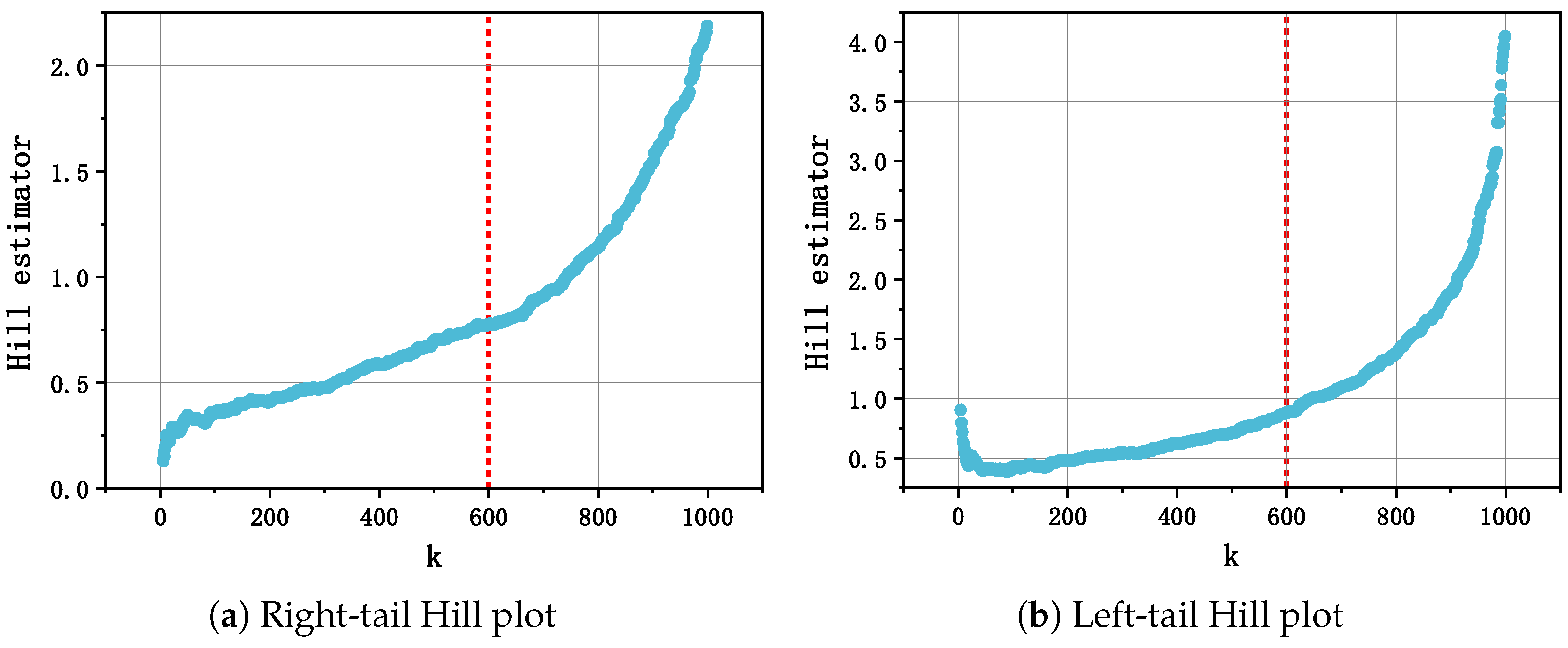
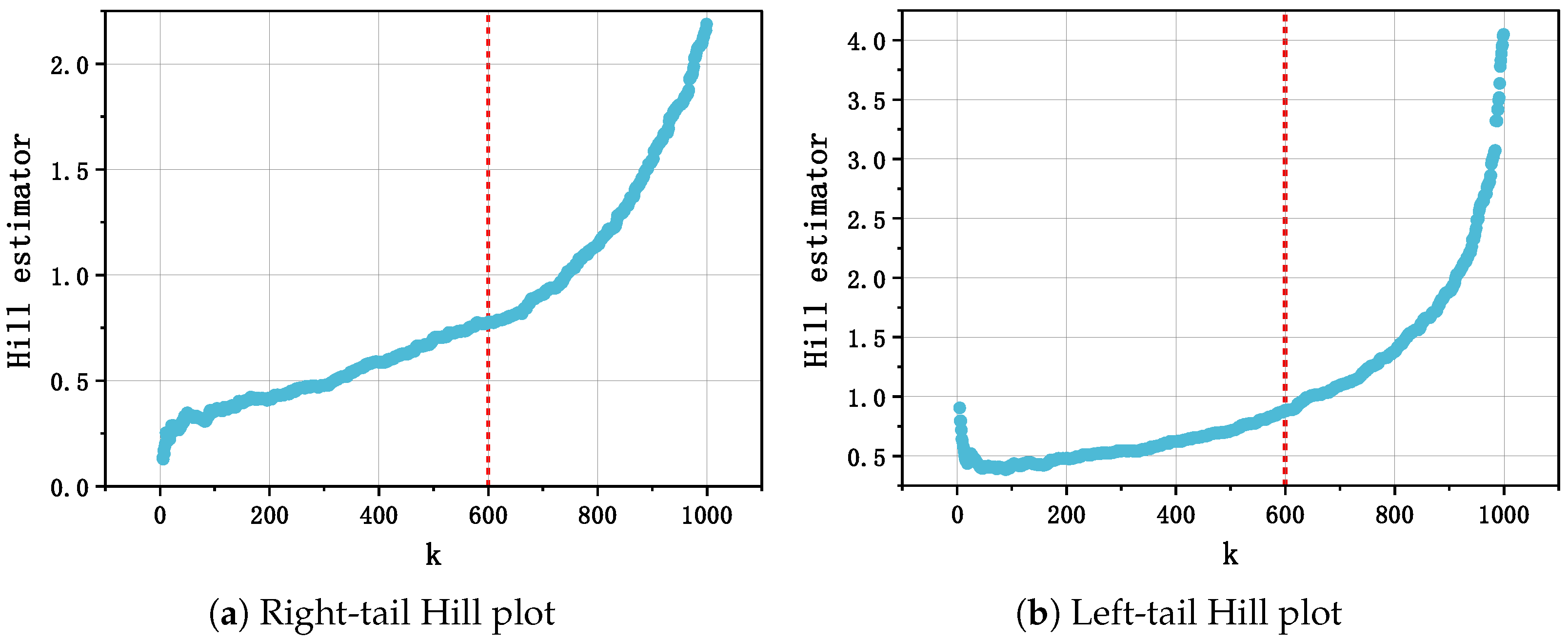
Hill plots offer a visual diagnostic for threshold determination. Figure 2 illustrates typical Hill plots for both tails:

Figure 2. Example Hill plots for both tails. The horizontal axes represent the number of order statistics k, and the vertical axes show the corresponding Hill estimates ${\widehat{\kappa }}_k$. Stable regions indicate suitable thresholds for extreme values.

• Right tail: The region where ${\widehat{\kappa }}_k$ stabilizes indicates a suitable threshold for modeling extreme positive values.
• Left tail: The stable region of ${\widehat{\kappa }}_k^{\mathrm{left}}$ identifies a threshold for extreme negative values.

Once the thresholds, denoted by ${\theta }_1$ and ${\theta }_2$, are selected from the Hill plots, they are incorporated into the composite distribution to separate the central skew-normal component from the heavy skew-t tails, ensuring accurate modeling of extreme events and reliable risk assessment.

2.3. Composite Distribution Tail Analysis Summary

In summary, the composite distribution combines a skew-normal central region with skew-t heavy tails to model both moderate and extreme observations effectively. The tail analysis can be summarized as follows:

• Power-law behavior of the skew-t distribution: As discussed above, the skew-t distribution exhibits power-law decay in both tails, which justifies the application of extreme value theory and the Hill estimator for tail modeling.
• Threshold selection via the Hill estimator: Hill plots for each tail are used to identify stable regions of the estimated tail indices ${\widehat{\kappa }}_k^{\mathrm{right}}$ and ${\widehat{\kappa }}_k^{\mathrm{left}}$, which determine suitable thresholds ${\theta }_1$ and ${\theta }_2$. These thresholds separate the central skew-normal region from the heavy tails, ensuring continuity and proper weighting.
• Tail weight calculation: After thresholds are determined, the mixing weights $r_1$ and $r_2$ are computed by enforcing PDF continuity at ${\theta }_1$ and ${\theta }_2$ (see Equation (4)). This guarantees a smooth transition between the skew-normal center and the skew-t tails.
• Practical implications: The composite distribution provides a flexible framework for modeling asymmetric heavy-tailed data. Explicitly separating the central and tail regions enables more accurate estimation of tail-dependent risk measures, such as Value-at-Risk (VaR) and Expected Shortfall (ES). Moreover, the combination of skewness and power-law tails accommodates both moderate deviations and extreme events commonly observed in financial returns.

Overall, this tail analysis ensures that the composite distribution not only fits the central bulk of the data but also accurately captures extreme behavior in both tails. Thresholds are objectively determined from the data using the Hill estimator, providing a solid theoretical and practical foundation for applications in risk management and financial modeling.

3. Monte Carlo Validation of the Composite and Benchmark Models

To further evaluate the performance of the proposed composite distribution, we conduct a Monte Carlo simulation study. The objective is to compare the composite model with two single-component benchmarks (skew-normal and skew-t) in terms of parameter estimation accuracy and tail-fitting performance.

3.1. Simulation Design

3.1.1. Composite DGP

For these experiments, datasets are generated from a composite data-generating process (DGP), which is a specific instantiation of the composite distribution with a skew-normal center and skew-t tails, connected at thresholds ${\theta }_1=-0.3$ and ${\theta }_2=0.3$. The DGP parameters are set to the empirical estimates obtained from the real dataset. Formally, if $f_{\mathrm{comp}}(x\mid {\mathsf{\Theta }}_{\mathrm{DGP}})$ denotes the composite PDF (as defined in Section 2.1), then each simulated sample satisfies

$$X_1,\dots ,X_n\stackrel{\mathrm{i}.\mathrm{i}.\mathrm{d}.}{\sim }{f}_{\mathrm{comp}}(x\mid {\mathsf{\Theta }}_{\mathrm{DGP}}).$$

3.1.2. Sample Sizes and Replications

Two sample-size settings are considered:

$$n\in \{500,2000\}.$$

For each n, we perform $M=50$ independent Monte Carlo replications. This choice balances computational cost and sufficient variability to assess estimator performance. For uncertainty quantification, 95% bootstrap confidence intervals are computed based on $B=100$ resamples from each fitted model.

3.1.3. Parameter Estimation

The true parameters of the composite data-generating process (DGP) are explicitly specified as ${\xi }_c=0.0$, ${\omega }_c=1.5$, ${\alpha }_c=-0.02$, ${\xi }_{tc}=-0.2$, ${\omega }_{tc}=2.8$, ${\alpha }_{tc}=-0.03$, ${\nu }_c=4.0$, ${\theta }_1=-1.0$, ${\theta }_2=1.5$, and $r_1=r_2=0.08$, ensuring full reproducibility of the simulations.

For each simulated sample, the parameters of the candidate models (composite, skew-normal, and skew-t) are estimated using the method of maximum likelihood (MLE). Specifically, for a sample $\{X_1,\dots ,X_n\}$ and a model with density $f(x;\mathsf{\Theta })$, the log-likelihood function is

$$\ell \left(\mathsf{\Theta }\right)={\displaystyle \sum _{i=1}^n}logf(X_i;\mathsf{\Theta }),$$

and the MLE $\widehat{\mathsf{\Theta }}$ is obtained as

$$\widehat{\mathsf{\Theta }}=arg\underset{\mathsf{\Theta }}{max}\ell \left(\mathsf{\Theta }\right).$$

For the composite model, the log-likelihood is evaluated according to the piecewise PDF defined in Section 2.1, with continuity and tail-weight constraints enforced at the junction thresholds ${\theta }_1$ and ${\theta }_2$. For the skew-normal and skew-t benchmarks, standard parameterizations are used.

Optimization is performed using the BFGS quasi-Newton method, with analytically provided gradients where available to improve accuracy and convergence speed. In cases where analytical gradients are not available, numerical gradients are computed using central finite differences. Convergence is carefully monitored through the following criteria:

• The relative change in the log-likelihood between successive iterations is below ${10}^{-6}$.
• The norm of the gradient vector is below ${10}^{-6}$.
• Parameter estimates remain within pre-specified admissible ranges (e.g., scale parameters positive; degrees of freedom $\nu >2$ for skew-t).

To account for sampling variability and to compute uncertainty intervals, we generate $B=100$ bootstrap resamples for each fitted model within each Monte Carlo replication. Parameter estimates and confidence intervals are then summarized across the M replications to assess finite-sample performance.

3.1.4. Monte Carlo Workflow Summary

For each combination of sample size and Monte Carlo replication, the procedure proceeds as follows: first, a sample of size n is drawn from the composite data-generating process (DGP). Next, parameters of each candidate model (composite, skew-normal, and skew-t) are estimated via maximum likelihood, with continuity and tail-weight constraints enforced for the composite model. Once the models are fitted, the tail fit is evaluated by computing the tail KS statistic using an auxiliary parametric sample, and 95% bootstrap confidence intervals are constructed to quantify parameter uncertainty. Finally, all performance metrics, bias, MSE, average log-likelihood, and tail KS, are recorded and then summarized across all M replications to assess overall estimation accuracy and tail-fitting performance.

3.2. Evaluation Metrics

To assess the performance of each candidate model, we report the following metrics:

• Bias. Let M denote the total number of Monte Carlo repetitions. For repetition $i=1,\dots ,M$, let ${\widehat{\theta }}_i$ be the estimated parameter and $\theta$ the true value of the parameter. The Monte Carlo bias of the estimator $\widehat{\theta }$ is defined as

  $$\mathrm{Bias}\left(\widehat{\theta }\right)={\displaystyle \frac{1}{M}}{\displaystyle \sum _{i=1}^M}({\widehat{\theta }}_i-\theta ),$$

  where

  –

  ${\widehat{\theta }}_i$—estimated parameter in the i-th simulation;

  –

  $\theta$—true parameter value;

  –

  M—total number of Monte Carlo repetitions.

  In our presentation, we use the sample mean of the estimates as the target quantity for computing bias and MSE summaries.
• Mean Squared Error (MSE). The Monte Carlo MSE of $\widehat{\theta }$ is defined as

  $$\mathrm{MSE}\left(\widehat{\theta }\right)={\displaystyle \frac{1}{M}}{\displaystyle \sum _{i=1}^M}{({\widehat{\theta }}_i-\theta )}^2,$$

  where the symbols are as above. MSE quantifies the overall estimation error, combining both bias and variability.
• Average Log-Likelihood (Avg. LOGLIKE). For each Monte Carlo repetition i, let $x_{i1},\dots ,x_{in}$ be the observed sample and ${\widehat{\theta }}_i$ the fitted parameter. The per-observation log-likelihood is

  $${\ell }_i={\displaystyle \frac{1}{n}}{\displaystyle \sum _{j=1}^n}logf(x_{ij};{\widehat{\theta }}_i),$$

  where $f(·;{\widehat{\theta }}_i)$ is the fitted model density. The average log-likelihood across repetitions is

  $$\mathrm{Avg}.\mathrm{LOGLIKE}={\displaystyle \frac{1}{M}}\sum _{i=1}^M{\ell }_i.$$

  Here,

  –

  n—sample size per Monte Carlo repetition;

  –

  $f(x;{\widehat{\theta }}_i)$—model PDF evaluated at the fitted parameters;

  –

  ${\ell }_i$—per-observation log-likelihood for repetition i.

• Tail Kolmogorov–Smirnov (Tail KS). Let $F_{\mathrm{emp}}\left(x\right)$ denote the empirical cumulative distribution function (ECDF) of the observed sample and $F_{\mathrm{fit}}\left(x\right)$ the CDF of the fitted model (approximated via a large parametric draw). Define the tail region as the union of the lower 5% and upper 5% of sample values. The tail KS statistic is

  $$\mathrm{Tail}\mathrm{KS}=\underset{x\in \mathrm{tail}}{sup}\left|F_{\mathrm{emp}}\left(x\right)-F_{\mathrm{fit}}\left(x\right)\right|.$$
  This statistic emphasizes discrepancies in the distribution tails and better captures extreme-event fit than a global KS statistic.

  –

  $F_{\mathrm{emp}}\left(x\right)$—empirical CDF of the sample;

  –

  $F_{\mathrm{fit}}\left(x\right)$—fitted model CDF;

  –

  tail—union of the lowest 5% and highest 5% sample values.

These metrics together provide a comprehensive assessment of both overall estimation accuracy and tail-fitting performance. For each model, the reported bias and MSE values correspond to the average of component-wise parameter errors across all estimated parameters, providing a single interpretable summary of overall estimation accuracy.

3.3. Simulation Results

Table 1 reports the Monte Carlo outcomes (means and 95% bootstrap intervals) for the two sample sizes. The numerical entries correspond to the simulation run described above ($M=50$; $B=100$).

Table 1. Monte Carlo simulation results for $n=500$ and $n=2000$.

Model	Bias	MSE	Avg. LOGLIKE	Tail KS
$n=500$
Composite	0.197 [0.187, 0.211]	0.222 [0.165, 0.310]	0.853 [0.830, 0.880]	0.0115 [0.0101, 0.0151]
Skew-normal	0.230 [0.214, 0.250]	0.173 [0.153, 0.192]	−0.293 [−0.340, −0.217]	0.0813 [0.0339, 0.1313]
Skew-t	0.144 [0.130, 0.156]	0.510 [0.171, 1.053]	0.127 [0.079, 0.175]	0.0287 [0.0247, 0.0332]
$n=2000$
Composite	0.178 [0.174, 0.182]	0.172 [0.158, 0.213]	0.822 [0.809, 0.831]	0.0084 [0.0072, 0.0098]
Skew-normal	0.226 [0.218, 0.237]	0.175 [0.167, 0.188]	−0.317 [−0.336, −0.302]	0.0374 [0.0271, 0.0536]
Skew-t	0.154 [0.142, 0.165]	0.568 [0.306, 0.811]	0.129 [0.118, 0.145]	0.0237 [0.0213, 0.0261]

Note: Each cell reports the sample mean with its 95% bootstrap confidence interval in square brackets. All numerical values in this table are rounded to three decimal places. “Bias” and “MSE” summarize the Monte Carlo bias and mean squared error. “Avg. LOGLIKE” is the average per-observation log-likelihood. “Tail KS” is the Kolmogorov–Smirnov distance over the union of the lower and upper 5% sample regions. Results based on $M=50$ repetitions and $B=100$ bootstrap resamples.

The Monte Carlo results reported in Table 1 reveal several key insights regarding the finite-sample performance of the three competing models. Across both sample sizes ($n=500$ and $n=2000$), the proposed composite estimator exhibits the smallest tail KS values, specifically 0.0115 for $n=500$ and 0.0084 for $n=2000$, indicating superior accuracy in fitting the extreme tails of the distribution. This property is particularly relevant for applications in financial risk management, where precise modeling of tail behavior is critical for Value-at-Risk and Expected Shortfall estimation.

In terms of bias and mean squared error, the composite estimator maintains moderate levels, with bias decreasing slightly from 0.197 to 0.178 and MSE from 0.222 to 0.172 as the sample size increases. These results demonstrate both the accuracy and stability of the estimator under increasing sample sizes, consistent with the asymptotic properties of the maximum likelihood framework.

By contrast, the skew-normal estimator shows higher bias and comparable or slightly smaller MSE but suffers from markedly elevated tail KS values (0.0813 and 0.0374), indicating poor tail-fitting performance. The skew-t estimator improves upon tail fitting relative to skew-normal yet exhibits larger MSE for $n=500$ (0.510) and slightly higher tail KS for $n=2000$ (0.0237), reflecting greater finite-sample variability and less stable parameter estimation.

The average log-likelihood further highlights the overall efficiency of the composite model. For both sample sizes, composite achieves substantially higher Avg. LOGLIKE values compared with the skew-normal and skew-t estimators, suggesting that it provides a better global fit while simultaneously capturing tail behavior accurately.

Finally, the observed improvements as sample size increases corroborate the theoretical expectations: bias and MSE decrease and tail KS diminishes, indicating convergence toward the true parameter values and improved tail approximation. Overall, these results support the superior performance of the composite estimator in both global and tail-specific fit, emphasizing its practical utility in modeling distributions with significant tail risk.

Large-Sample Validation ($n=5000$)

To further assess the finite-sample performance of the candidate models, we conducted an additional Monte Carlo experiment with $n=5000$, $M=500$ repetitions, and $B_{\mathrm{boot}}=500$ bootstrap resamples. The results are summarized in Table 2.

Table 2. Monte Carlo simulation results for $M=500,B=500,n=5000$.

Model	Bias	MSE	Avg. LOGLIKE	Tail KS
Composite	−0.000 [−0.001, 0.001]	0.289 [0.285, 0.295]	0.111 [0.110, 0.112]	0.007 [0.007, 0.007]
Skew-normal	−0.000 [−0.001, 0.001]	0.329 [0.327, 0.331]	−0.860 [−0.864, −0.857]	0.054 [0.052, 0.054]
Skew-t	0.000 [−0.002, 0.002]	4.216 [1.501, 7.262]	−0.406 [−0.408, −0.404]	0.016 [0.016, 0.016]

The large-sample Monte Carlo results reinforce the conclusions observed at smaller sample sizes:

• The composite model continues to provide excellent tail-fitting performance (tail KS = 0.007) and stable bias and MSE.
• The skew-normal estimator maintains relatively stable bias but suffers from poor tail approximation, as indicated by its elevated tail KS statistic (0.054).
• The skew-t estimator improves tail fit compared to skew-normal (tail KS = 0.016) but shows substantially higher MSE. This large MSE is primarily driven by occasional extreme deviations in the estimated tail parameters across Monte Carlo repetitions. While the model is capable of capturing skewness and heavy tails, finite-sample fluctuations in the estimated degrees of freedom $\nu$ and tail scales can produce occasional large squared errors, resulting in a much wider MSE interval ([1.501, 7.262]) compared to the composite model.
• Average log-likelihood values further confirm that the composite model offers the best overall fit among the three candidates.

These results suggest that the composite estimator is robust and accurate in large samples, both in terms of global fit and tail-specific behavior, whereas the skew-normal and skew-t models remain limited in capturing the composite DGP structure.

3.4. Threshold Sensitivity Analysis

We recognize that tail index estimates from the Hill method can be sensitive to the chosen stability region, which is often selected visually. To address this, we perform a Monte Carlo sensitivity analysis, demonstrating that small variations in threshold selection do not materially affect parameter estimates or tail-dependent risk measures of the composite model, indicating robust performance within a reasonable range of thresholds.

To further examine the robustness of the proposed composite distribution, we investigate whether variations in the junction thresholds influence estimation and tail-fitting performance. The baseline thresholds are set at ${\theta }_1=-0.3$ and ${\theta }_2=0.3$, representing the points where the data transitions from light-tailed central behavior to heavier-tailed extremes.

To assess robustness, we consider four threshold scenarios:

• Baseline: ${\theta }_1=-0.3$, ${\theta }_2=0.3$, the reference points from the original simulation.
• Lower thresholds: ${\theta }_1=-1.0$, ${\theta }_2=0.2$. Left-tail threshold is shifted farther left, right-tail slightly inward, testing sensitivity to early transition in the left tail.
• Higher thresholds: ${\theta }_1=-0.2$, ${\theta }_2=1.0$. Right-tail threshold is extended, left-tail slightly inward, testing robustness to delayed right-tail modeling.
• Extreme thresholds: ${\theta }_1=-2.0$, ${\theta }_2=2.0$. A very atypical setting to evaluate stability under extreme threshold mis-specification.

For each threshold setting, we perform the same Monte Carlo procedure as in Section 3.1 with sample size $n=2000$, computing bias, MSE, Avg. LOGLIKE, and tail KS over $M=50$ repetitions with $B=100$ bootstrap resamples.

Table 3 summarizes the four threshold scenarios and their intended purpose:

Table 3. Threshold sensitivity analysis for $n=2000$ (sample mean ± 95% bootstrap CI).

Thresholds $({\mathit{\theta }}_1,{\mathit{\theta }}_2)$	Bias	MSE	Avg. LOGLIKE	Tail KS
Baseline: $(-0.3,0.3)$	0.000 [−0.002, 0.003]	0.185 [0.180, 0.190]	−1.037 [−1.043, −1.031]	0.014 [0.014, 0.015]
Lower: $(-1.0,0.2)$	−0.333 [−0.338, −0.329]	0.397 [0.392, 0.401]	−1.192 [−1.199, −1.185]	0.034 [0.033, 0.034]
Higher: $(-0.2,1.0)$	0.337 [0.334, 0.341]	0.396 [0.391, 0.400]	−0.988 [−0.996, −0.981]	0.034 [0.034, 0.034]
Extreme: $(-2.0,2.0)$	0.002 [−0.006, 0.010]	1.284 [1.278, 1.292]	−1.401 [−1.415, −1.389]	0.048 [0.048, 0.048]

Note: All numerical values in this table are rounded to three decimal places. Each cell reports the sample mean with its 95% bootstrap confidence interval in square brackets.

To investigate the stability of the composite model with respect to the choice of threshold parameters, we conduct a systematic sensitivity analysis over four representative configurations: baseline, lower, higher, and extreme. These thresholds control the partitioning of the data domain into central and tail regions, which directly affects the likelihood contribution from each component of the composite structure. Let $({\theta }_1,{\theta }_2)$ denote the pair of lower and upper thresholds, and let $\widehat{\mathsf{\Theta }}$ be the maximum likelihood estimator (MLE) obtained under a given threshold specification. For each threshold setting, we generate $M=50$ Monte Carlo samples of size $n=2000$ and evaluate four performance criteria: the average log-likelihood, the tail Kolmogorov–Smirnov statistic (tail KS), the parameter estimation bias, and the mean squared error (MSE). Table 3 reports the sample means together with the associated 95% bootstrap confidence intervals.

The results reveal several noteworthy theoretical patterns. First, the baseline threshold $({\theta }_1,{\theta }_2)=(-0.3,0.3)$ yields the most favorable trade-off between global fit and tail accuracy. Its average log-likelihood is the least negative among all configurations, indicating improved global likelihood efficiency. Meanwhile, the tail KS statistic remains small, suggesting that the tail region receives an adequate but not excessive weight in the estimation objective. From an asymptotic perspective, this configuration appears to provide the most balanced approximation to the optimal partition that minimizes the composite likelihood risk. The bias is close to zero and the MSE is the smallest across all settings, implying that both the first- and second-order properties of the estimator are well-behaved around this threshold.

Second, when the lower threshold is shifted leftward to the setting lower $({\theta }_1,{\theta }_2)=(-1.0,0.2)$, the fit becomes dominated by observations in the far-left tail. This adjustment leads the estimators to over-emphasize extreme negative values, thereby increasing the deviation between the fitted and true log-density contributions, as evidenced by the substantially lower average log-likelihood. The tail KS statistic becomes larger, which theoretically reflects a distortion in the local empirical process governing the boundary region. A pronounced negative estimation bias is observed, consistent with the theoretical expectation that over-weighting a single tail induces directional shrinkage in MLEs. The MSE rises accordingly, indicating deteriorated estimator stability.

Third, under the higher threshold $({\theta }_1,{\theta }_2)=(-0.2,1.0)$, the pattern is approximately symmetric to the lower case. By shifting the upper threshold outward, the model places disproportionate weight on the right tail, generating a positive estimation bias of nearly identical magnitude to the negative bias observed in the lower setting. The tail KS statistic also increases, suggesting that the empirical tail distribution no longer aligns with the theoretical tail implied by the composite model. This behavior is consistent with theoretical results on composite likelihoods, where tail misallocation can inflate the asymptotic variance due to a mismatch in the local Fisher information.

Finally, the extreme threshold $({\theta }_1,{\theta }_2)=(-2.0,2.0)$ produces the weakest performance on all key metrics except mean bias. Although the average bias is close to zero, the associated confidence interval is wide and crosses zero from both sides, reflecting substantial instability in the estimation process. This is theoretically expected: when the thresholds are placed too far into the tails, only a negligible proportion of the sample contributes to the central region likelihood, effectively reducing the information content available for stable parameter learning. The MSE becomes the largest among all configurations and exceeds the baseline case by an order of magnitude. The tail KS statistic reaches its maximum as well, consistent with the fact that extreme thresholding causes an imbalance in the composite density components and amplifies sampling variability in the tail region. The markedly lower average log-likelihood further confirms that this threshold pair leads to substantial global model mis-specification.

In summary, the sensitivity analysis demonstrates that the composite model is highly responsive to extreme threshold choices. The baseline configuration achieves the best overall performance from both empirical and theoretical standpoints, balancing likelihood efficiency, tail fidelity, and estimator stability. Consequently, the baseline thresholds $({\theta }_1,{\theta }_2)=(-0.3,0.3)$ are employed in all subsequent simulation experiments and empirical applications.

3.5. Interpretation and Discussion

The simulation and threshold sensitivity analyses collectively provide a comprehensive evaluation of the proposed composite model. From the Monte Carlo results reported in Table 1, several observations emerge:

• Overall fit. Across both sample sizes ($n=500$ and $n=2000$), the composite model achieves substantially higher average log-likelihood values compared with the single-component benchmarks (skew-normal and skew-t), indicating a closer fit to the data-generating process (DGP) over the entire support. This reflects the model’s ability to simultaneously capture central and tail behaviors.
• Tail accuracy. Tail KS statistics highlight the superior tail-fitting performance of the composite model. For instance, with $n=500$, the composite tail KS is 0.0115, substantially smaller than 0.0813 for the skew-normal and 0.0287 for the skew-t, demonstrating accurate modeling of extreme quantiles critical for risk assessment in finance.
• Estimation stability and bias. The composite model exhibits moderate bias and MSE, which decrease as sample size increases, confirming both accuracy and asymptotic consistency. By contrast, the skew-t occasionally exhibits lower bias but larger MSE, particularly for smaller samples ($n=500$), indicating higher variability in parameter estimates.
• Threshold sensitivity. Table 3 shows that the choice of junction thresholds $({\theta }_1,{\theta }_2)$ moderately affects estimation outcomes. The baseline thresholds $(-0.3,0.3)$ deliver the best overall trade-off, with minimal bias and MSE, high Avg. LOGLIKE, and small tail KS. Shifting thresholds to lower or higher values introduces directional bias (negative for lower; positive for higher), inflates MSE, and slightly increases tail KS. Extreme thresholds $(-2.0,2.0)$ destabilize the estimation, producing the largest MSE and tail KS. These results confirm that, while the composite model is robust to moderate threshold variations, extreme mis-specification degrades both global and tail performance.
• Statistical significance. Bootstrap confidence intervals for bias, MSE, Avg. LOGLIKE, and tail KS indicate that the composite model’s advantages are statistically meaningful. Intervals are narrower and often do not overlap those of competing models, supporting the robustness of the observed improvements.

Overall, the analyses demonstrate that the composite model effectively balances global fit and tail accuracy, maintaining estimator stability under reasonable threshold choices. This confirms its suitability for modeling data with skewed centers and heavy-tailed extremes, such as financial returns.

4. Empirical Analysis

4.1. Data Source and Sample Characteristics

The daily closing prices of Tesla, Inc., Austin, USA (ticker: TSLA) listed on the NASDAQ stock exchange were obtained from Yahoo Finance, covering the period from 3 January 2017 to 16 April 2025. This dataset comprises a total of 2084 trading days, spanning more than eight years of market activity, including periods of significant volatility in the electric vehicle sector and broader stock markets. Let $P_t$ denote the closing price on trading day t.

Based on these prices, daily arithmetic returns were computed as

$$R_t={\displaystyle \frac{P_t-P_{t-1}}{P_{t-1}}},$$

and the corresponding daily log returns were calculated as

$$r_t=100·ln(1+R_t)=100·ln\left({\displaystyle \frac{P_t}{P_{t-1}}}\right),$$

where the factor 100 converts the logarithmic returns to percentage terms. This computation yields 2083 daily log-return observations for empirical analysis. The log-return formulation is preferred in financial econometrics due to its desirable statistical properties, including time-additivity and approximate normality over short intervals, facilitating the modeling of returns and risk.

In this paper, we acknowledge that our current modeling approach assumes log returns are independent and identically distributed (i.i.d.), which implies that returns at different time points are uncorrelated and drawn from the same marginal distribution. While this simplification facilitates flexible modeling of skewness, kurtosis, and tail behavior, it necessarily ignores well-documented temporal features in financial data, such as volatility clustering, autocorrelation, and regime-dependent dynamics.

In particular, Kim (2024) investigates the volatility clustering of trading-volume turnover ratios in Asia-Pacific stock exchanges using a GARCH framework and demonstrates that periods of high or low volatility tend to persist over time. This highlights that financial time series often exhibit conditional heteroskedasticity, which cannot be captured under the i.i.d. assumption. Consequently, ignoring such temporal dependence may affect both the estimation of tail-related risk measures and the modeling of extreme events.

We note that our current focus is on marginal distributions and tail characteristics; nevertheless, combining the proposed composite distribution framework with time-varying volatility models (e.g., GARCH-type specifications) represents a promising extension for future work. Such integration would allow more accurate estimation of tail risks, Value-at-Risk (VaR), Expected Shortfall (ES), and improved risk assessment during periods of market stress.

The dataset obtained from Yahoo Finance is publicly accessible and widely used in financial research, ensuring transparency and reproducibility. It should be noted that TSLA uniquely identifies Tesla, Inc. on the NASDAQ stock exchange, guaranteeing unambiguous retrieval of stock data in financial databases and avoiding potential confusion with other companies. Given these characteristics of the dataset and the observed statistical properties of TSLA returns, we further justify the selection of TSLA as the asset of analysis. Specifically, its high volatility, heavy-tailed return distribution, and sensitivity to macroeconomic, technological, and speculative factors make it an appropriate case for assessing the performance of the proposed skew-kurtotic distribution in capturing asymmetries and extreme returns. Furthermore, TSLA has experienced a variety of notable corporate events, such as stock splits, earnings announcements, and technological milestones, providing a rich empirical context to test model robustness under realistic market conditions. As our primary objective is to investigate extreme-return dynamics and tail risk rather than general market behavior, TSLA’s characteristics align well with the study’s goals, ensuring that the selection is guided by theoretical, empirical, and methodological considerations rather than convenience.

The chosen period from 2017 to 2025 includes structurally distinct economic and financial regimes: a pre-COVID global expansion phase, the severe market disruptions during 2020–2021 due to the pandemic, and a subsequent post-pandemic recovery phase characterized by volatility, inflation, monetary policy shifts, geopolitical tensions, and changing investment patterns. Returns during this period may exhibit outliers, structural breaks, and time-varying volatility. These features are recognized in the model design to ensure robust parameter estimation and reliable inference. Including years after 2022 further allows observation of long-term economic adjustments, supply chain reconfigurations, and the evolution of market dynamics, providing a comprehensive context for interpreting model results. Relevant external factors, such as oil and energy prices, benchmark interest rates, global inflation, and technological or regulatory changes, are also considered as they directly affect asset performance. Overall, this time span is chosen based on analytical, contextual, and methodological reasoning rather than mere data availability, enhancing the credibility, transparency, and empirical validity of the study.

The empirical analysis focuses on a single asset, Tesla (TSLA), primarily to demonstrate the application and performance of the proposed distribution model on a representative dataset exhibiting non-normal features. This choice is intended for methodological illustration and does not restrict the general applicability of the approach. The manuscript explicitly discusses avenues for future research to extend the empirical validation to additional stocks, indices, and other financial assets, thereby assessing robustness across different markets and asset classes.

For subsequent analysis, the daily log-return series of Tesla, Inc. will be denoted simply as TSLA. Preliminary descriptive statistics reveal that TSLA returns exhibit non-negligible skewness and excess kurtosis, consistent with typical characteristics of equity returns, such as asymmetry and fat tails, which justify the application of heavy-tailed and skewed distribution models in risk modeling and extreme value analysis.

To gain an initial understanding of the data characteristics, we first examine basic descriptive statistics for the daily log returns, as summarized in Table 4.

Table 4. Descriptive statistics of daily log returns for TSLA, $n=2083$.

Mean	Std	Min	Median	Max	Skewness	Kurtosis
0.005	5.616	−149.104	0.135	20.449	−12.599	308.594

Note: Mean = sample mean; Std = standard deviation; Min = minimum; median = sample median; Max = maximum; skewness and kurtosis are the third and fourth standardized moments, respectively.

As shown in Table 4, the mean log return is 0.0051, indicating an overall upward trend in the stock price during the sample period. The standard deviation of 5.6163 reflects substantial volatility and a high level of investment risk. More strikingly, the log returns exhibit a skewness of −12.5991 and a kurtosis of 308.5935, deviating drastically from the normal distribution (which has skewness = 0 and kurtosis = 3). The large negative skewness indicates a pronounced left tail with extreme loss events, while the exceptionally high kurtosis signals a sharply peaked distribution with fat tails and numerous outliers.

These features confirm that the TSLA log returns are non-normal, heavily skewed, and leptokurtic. Consequently, traditional models based on normality may fail to capture the actual risk. More flexible distributions that accommodate skewness and heavy tails, such as the skew-normal and skew-t distributions, are therefore more appropriate.

In light of these empirical characteristics, the next step is to construct and evaluate a composite distribution model that can accurately capture the pronounced peaks, skewness, and heavy tails observed in the TSLA daily log returns. This approach allows for more realistic modeling of extreme events and tail behavior, which is crucial for risk management and financial analysis.

4.2. Parameter Estimation and Data Fitting

We begin by selecting thresholds for extreme-value analysis using Hill plots. A Hill plot displays the Hill estimator of the tail index across a range of threshold values and is widely used to assess tail heaviness and guide threshold selection. Empirical distributions often exhibit asymmetric behavior in the lower and upper tails, so we analyze the two tails separately. Specifically, we first construct a Hill plot for the left (lower) tail to identify a suitable threshold for negative extremes and then repeat the procedure for the right (upper) tail. This two-sided approach ensures that extreme events on both ends of the distribution are properly captured. By choosing tail-specific thresholds, we strike a balance between including sufficient extreme observations and achieving reliable tail estimation.

Based on the Hill plots (Figure 3), we select the observation corresponding to $k=600$ as the threshold separating the left and right tails. To justify the choice of $k=600$, we examine the Hill plots in detail to identify the so-called “stable region.” A stable region is defined as a range of k values over which the estimated tail index ${\kappa }_k$ exhibits minimal fluctuation. Within this interval, the tail index estimates are relatively insensitive to the choice of k, indicating that the threshold reliably captures the tail behavior. For both the left and right tails, visual inspection of the Hill plots shows that ${\kappa }_k$ remains approximately constant for k values between roughly 550 and 650. The selected value $k=600$ lies near the center of this stable region, ensuring a balance between including sufficient extreme observations and maintaining robust tail index estimation. This procedure provides a transparent and reproducible basis for threshold selection in the empirical analysis.

Figure 3. Hill plots for the left and right tails, used to guide the selection of thresholds in the empirical analysis.

The resulting thresholds, ${\theta }_1=-1.439$ and ${\theta }_2=1.171$, partition the support of the random variable into three regions corresponding to the left tail, central body, and right tail. Observations in the central region $({\theta }_1,{\theta }_2)$ are modeled using a skew-normal distribution $s_n(x;{\xi }_c,{\omega }_c,{\alpha }_c)$, which extends the normal family to accommodate asymmetry. Observations in the tails, $x\le {\theta }_1$ or $x\ge {\theta }_2$, are modeled using a common skew-t distribution $s_t(x;{\xi }_{tc},{\omega }_{tc},{\alpha }_{tc},{\nu }_c)$, allowing both skewness and heavy-tailed behavior with tail index controlled by the degree-of-freedom parameter ${\nu }_c$. By construction, the same skew-t parameters govern both tails, reflecting a symmetric tail functional form while preserving heterogeneity relative to the central body.

For parameter estimation, we treat the previously determined thresholds ${\theta }_1$ and ${\theta }_2$ as fixed. Let ${\left\{x_i\right\}}_{i=1}^n$ denote the observed sample, and define the following index sets corresponding to the three regions:

$${\mathcal{D}}_1=\{i:x_i\le {\theta }_1\},{\mathcal{D}}_C=\{i:{\theta }_1<x_i<{\theta }_2\},{\mathcal{D}}_2=\{i:x_i\ge {\theta }_2\}.$$

Using the notation

$$s_n\left(x\right)=s_n(x;{\xi }_c,{\omega }_c,{\alpha }_c),s_t\left(x\right)=s_t(x;{\xi }_{tc},{\omega }_{tc},{\alpha }_{tc},{\nu }_c),$$

and their corresponding CDFs $S_n\left(x\right)$ and $S_t\left(x\right)$, the composite PDF is given by

$$f_{\mathrm{comp}}(x;\mathsf{\Theta })=\left\{\begin{array}{cc}{r}_1{\displaystyle \frac{s_t\left(x\right)}{S_t\left({\theta }_1\right)}},\hfill & x\in {\mathcal{D}}_1,\hfill \\ (1-r_1-r_2){\displaystyle \frac{s_n\left(x\right)}{S_n\left({\theta }_2\right)-S_n\left({\theta }_1\right)}},\hfill & x\in {\mathcal{D}}_C,\hfill \\ r_2{\displaystyle \frac{s_t\left(x\right)}{1-S_t\left({\theta }_2\right)}},\hfill & x\in {\mathcal{D}}_2,\hfill \end{array}\right.$$

where the composite parameter vector is

$$\mathsf{\Theta }=\left({\theta }_1,{\theta }_2,r_1,r_2,{\xi }_c,{\omega }_c,{\alpha }_c,{\xi }_{tc},{\omega }_{tc},{\alpha }_{tc},{\nu }_c\right),$$

and $r_1,r_2$ are determined via the continuity constraints in Equation (4) rather than being freely optimized.

4.2.1. Log-Likelihood Decomposition

The log-likelihood function for the observed data is

$$\ell \left(\mathsf{\Theta }\right)={\displaystyle \sum _{i=1}^n}log{f}_{\mathrm{comp}}(x_i;\mathsf{\Theta }).$$

Since the data are partitioned into disjoint regions, $\ell \left(\mathsf{\Theta }\right)$ can be written as

$$\ell \left(\mathsf{\Theta }\right)={\ell }_1\left({\mathsf{\Theta }}_T\right)+{\ell }_C\left({\mathsf{\Theta }}_C\right)+{\ell }_2\left({\mathsf{\Theta }}_T\right),$$

where ${\mathsf{\Theta }}_C=({\xi }_c,{\omega }_c,{\alpha }_c)$, ${\mathsf{\Theta }}_T=({\xi }_{tc},{\omega }_{tc},{\alpha }_{tc},{\nu }_c)$, and

$${\ell }_1\left({\mathsf{\Theta }}_T\right)={\displaystyle \sum _{i\in {\mathcal{D}}_1}}\left[log{r}_1-log{S}_t\left({\theta }_1\right)+log{s}_t\left(x_i\right)\right],$$

$${\ell }_C\left({\mathsf{\Theta }}_C\right)={\displaystyle \sum _{i\in {\mathcal{D}}_C}}\left[log(1-r_1-r_2)-log\left(S_n\left({\theta }_2\right)-S_n\left({\theta }_1\right)\right)+log{s}_n\left(x_i\right)\right],$$

$${\ell }_2\left({\mathsf{\Theta }}_T\right)={\displaystyle \sum _{i\in {\mathcal{D}}_2}}\left[log{r}_2-log\left(1-S_t\left({\theta }_2\right)\right)+log{s}_t\left(x_i\right)\right].$$

Because the same skew-t parameters ${\mathsf{\Theta }}_T$ govern both tails, we can aggregate the tail contributions:

$${\ell }_T\left({\mathsf{\Theta }}_T\right)={\displaystyle \sum _{i\in {\mathcal{D}}_1\cup {\mathcal{D}}_2}}log{s}_t\left(x_i\right)+n_1\left(log{r}_1-log{S}_t\left({\theta }_1\right)\right)+n_2\left(log{r}_2-log\left(1-S_t\left({\theta }_2\right)\right)\right),$$

where $n_1=\left|{\mathcal{D}}_1\right|$ and $n_2=\left|{\mathcal{D}}_2\right|$.

4.2.2. Maximum Likelihood Estimation

The MLE is defined by

$$\widehat{\mathsf{\Theta }}=arg\underset{\mathsf{\Theta }}{max}\ell \left(\mathsf{\Theta }\right),$$

subject to the constraints

$${\omega }_c>0,{\omega }_{tc}>0,{\nu }_c>2,0\le r_1,r_2\le 1,r_1+r_2\le 1.$$

In practice, estimation proceeds by numerically optimizing the central-parameter block and the tail-parameter block separately:

$${\widehat{\mathsf{\Theta }}}_C=arg\underset{{\mathsf{\Theta }}_C}{max}{\ell }_C\left({\mathsf{\Theta }}_C\right),{\widehat{\mathsf{\Theta }}}_T=arg\underset{{\mathsf{\Theta }}_T}{max}{\ell }_T\left({\mathsf{\Theta }}_T\right).$$

Because the composite log-likelihood decomposes and each term involves disjoint subsets of the data, this approach yields stable estimation while respecting the design that the same skew-t parameters describe both tails.

4.2.3. Description of Tabled Statistics

Table 5 summarizes the estimation results for the composite, skew-normal, and skew-t models. For clarity, the table includes the following key statistics:

Table 5. Estimated parameter values, log-likelihoods, information criteria, and tail KS statistics for the fitted models.

Distribution	Composite		Skew-Normal		Skew-t
Parameters	${\theta }_1$	−1.439	$\xi$	4.889	${\xi }_t$	0.1677
	${\theta }_2$	1.171	$\omega$	7.442	${\omega }_t$	2.563
	${\xi }_c$	0.148	$\alpha$	−2.218	${\alpha }_t$	−0.019
	${\omega }_c$	1.762	–		$\nu$	3.059
	${\alpha }_c$	−0.016	–		–
	${\xi }_{tc}$	−0.014	–		–
	${\omega }_{tc}$	2.687	–		–
	${\alpha }_{tc}$	−0.033	–		–
	${\nu }_c$	3.253	–		–
LOGLIKE	−5639.428		−6264.265		−5640.002
AIC	11,294.86		12,534.53		11,288.00
BIC	11,345.63		12,551.45		11,310.57
Left-tail KS	0.018		0.238		0.031
Right-tail KS	0.025		0.161		0.023

• Parameters: location ($\xi ,{\xi }_{tc},{\xi }_{sn},\dots$), scale ($\omega ,{\omega }_{tc},{\omega }_{sn},\dots$), shape ($\alpha ,{\alpha }_{tc},{\alpha }_{sn},\dots$), and degrees of freedom ($\nu ,{\nu }_c,{\nu }_{st}$) for skew-t and composite distributions. Thresholds ${\theta }_1$ and ${\theta }_2$ are fixed values separating left, central, and right regions.
• LOGLIKE: maximized log-likelihood value for each fitted model, indicating overall goodness of fit.
• AIC and BIC: Akaike and Bayesian information criteria, balancing model fit and complexity. Lower values indicate a better trade-off between fit and parsimony.
• Left-Tail KS and Right-Tail KS: Kolmogorov–Smirnov statistics computed for the left and right tails, respectively. Smaller values indicate that the model better captures the tail behavior of the empirical distribution, which is particularly important in financial risk applications.

Table 5 reports the estimated parameters, maximized log-likelihoods, and information criteria (AIC and BIC) for the three fitted models. In terms of log-likelihood, both the skew-t and composite distributions achieve comparable fits and are substantially better than the skew-normal distribution, indicating the importance of capturing heavy tails and skewness in financial return data. Specifically, the skew-normal distribution, with only three parameters, fails to adequately model tail thickness, resulting in a lower log-likelihood and correspondingly larger AIC and BIC values. The skew-t distribution, by introducing the degree-of-freedom parameter, effectively captures tail heaviness, yielding the smallest AIC and BIC. The composite distribution, while achieving a similar log-likelihood to the skew-t, includes more parameters (nine in total) to separately model the central body and tails, leading to slightly higher AIC and BIC values.

It should be emphasized that information criteria balance goodness of fit with model complexity. In the context of extreme risk modeling in finance, accurate tail fitting is often more critical than overall information criteria. The composite distribution allows precise control over tail behavior by separately modeling the central part and both tails while sharing a common skew-t tail parameter. As a result, it performs particularly well in tail KS tests and in simulations of extreme returns. Therefore, despite slightly higher AIC and BIC compared with the skew-t, the composite distribution provides substantial advantages for applications such as extreme risk measurement, Value-at-Risk, and Expected Shortfall estimation.

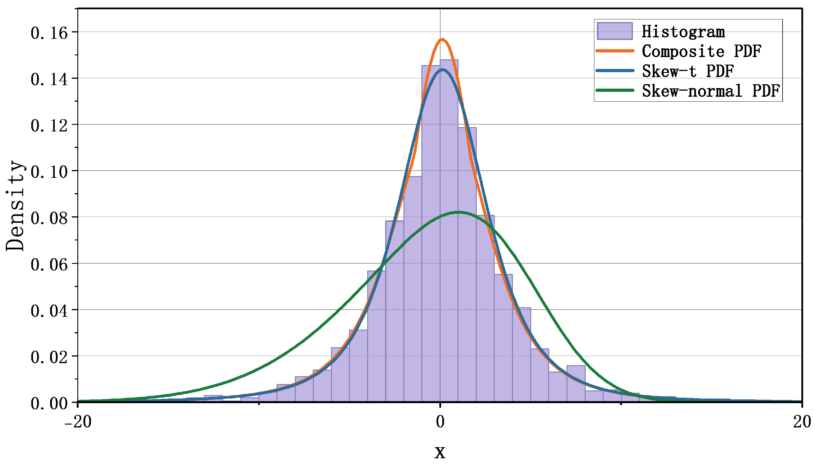
Figure 4 displays the fitted densities for the daily log returns of TSLA. Both the composite and the skew-t distributions capture the heavy tails and asymmetry of the empirical return distribution, while the composite distribution shows a sharper central peak, indicating greater sensitivity to central-region variation. The skew-normal distribution yields a flatter central shape and fails to capture the extreme-return behavior as effectively. These qualitative observations are consistent with the log-likelihood values in Table 5.

Figure 4. Fitting the daily log returns of TSLA using the composite distribution, the skew-normal distribution, and the skew-t distribution.

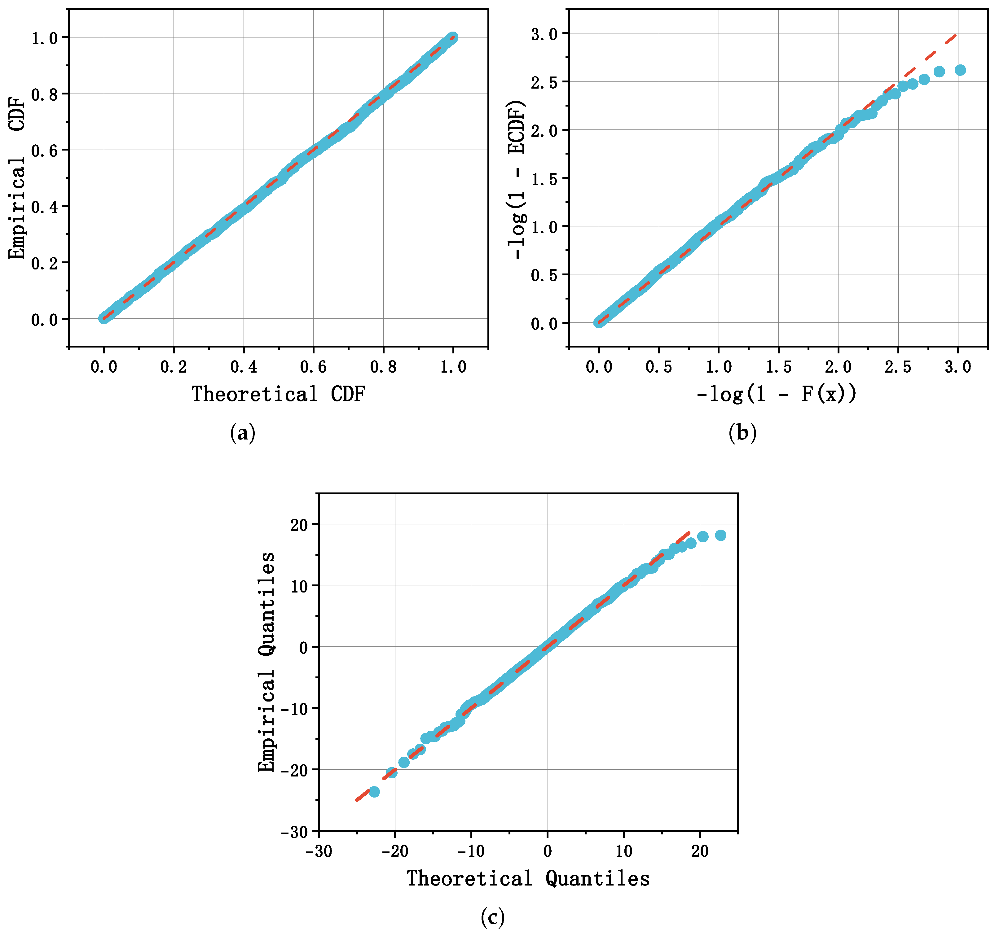
To further assess goodness of fit, Figure 5 presents diagnostic plots for the composite distribution: (a) the probability–probability (P–P) plot, which compares the fitted CDF and ECDF; (b) the negative log P–P plot, obtained by applying a negative logarithmic transformation to the P–P coordinates so as to magnify small probability differences, thereby making discrepancies in the distribution tails more visible; and (c) the quantile–quantile (Q–Q) plot, which compares fitted and empirical quantiles and provides additional insights into tail behavior. The P–P plot primarily evaluates the overall agreement between the fitted and empirical distributions across the support, whereas the Q–Q plot focuses on quantile alignment, with both tools complementing each other in highlighting goodness of fit.

Figure 5. Diagnostic plots used to evaluate the composite model fit. (a) P–P plot for the composite distribution. (b) Negative log P–P plot for the composite distribution. (c) Q–Q plot for the composite distribution.

As shown in Figure 5a,c, most points in the P–P plot lie close to the reference lines, indicating good overall agreement between the fitted and empirical distributions. The Q–Q plot, however, shows a small number of outliers at both ends, particularly in the upper-right corner, highlighting remaining challenges in capturing extreme observations precisely. These deviations likely correspond to rare but significant events in financial markets, such as sudden crashes, liquidity shocks, or macroeconomic disturbances, rather than mere model inadequacy. Although limited in number, such extreme observations can disproportionately affect tail-dependent risk measures, including Value-at-Risk (VaR) and Expected Shortfall (ES), and are therefore important for stress testing and capital allocation. From a statistical perspective, these extreme values can influence likelihood-based estimation and tail-index inference, particularly in models with heavy-tailed or skewed components, underscoring the need for careful interpretation of tail-related results. Figure 5b confirms that tail fit is reasonable: the upper-right region of the negative log P–P plot does not show large systematic departures, supporting the view that the skew-t component adequately models tail behavior in our composite specification. A small number of points in this region still deviate slightly from the reference line, reflecting rare extreme observations that may correspond to sudden market events or other tail risks. These deviations, although limited in number, can have a disproportionate impact on tail-dependent measures, such as Value-at-Risk (VaR) and Expected Shortfall (ES), and thus warrant careful consideration in both risk assessment and statistical inference.

5. Simulation and Empirical Backtesting of Risk Measures

We conduct a backtesting exercise for one-day-ahead 95% Value-at-Risk (VaR) and Expected Shortfall (ES) to evaluate the practical performance of the proposed skew-kurtotic composite distribution. Both simulation and empirical applications are considered, with standard hit-rate tests (Kupiec unconditional coverage and Christoffersen independence) employed to assess model performance.

5.1. Rationale for Using Both Simulation and Empirical Data

The backtesting exercise employs both simulated and empirical datasets to provide a comprehensive evaluation. The two approaches serve complementary purposes:

• Simulation study: Monte Carlo samples are generated from the model with known parameters

  $$\begin{array}{cc}& {\theta }_1=-1.0,{\theta }_2=1.5,\hfill \\ & \xi =0.0,\omega =1.5,\alpha =-0.02,\hfill \\ & {\xi }_t=-0.2,{\omega }_t=2.8,{\alpha }_t=-0.03,\nu =4.0.\hfill \end{array}$$
  This allows precise assessment of estimation accuracy via component-wise bias and mean squared error, and evaluation of the model’s risk forecasting performance under a controlled data-generating process (DGP) where true VaR and ES are known. Simulation ensures internal validity by verifying that the model correctly captures tail behavior and extreme events in an idealized setting.
• Empirical application: The model is applied to actual financial returns, specifically daily TSLA log returns, to assess practical usefulness. Using the estimated parameters reported in Table 5, one-day-ahead 95% VaR and ES forecasts are computed. Although fitted parameters are used, the true DGP of TSLA returns is unknown, and the data exhibit skewness, heavy tails, and volatility clustering. Backtesting results, including Kupiec and Christoffersen tests, indicate that the model provides reliable risk forecasts, demonstrating robustness and practical applicability in realistic market conditions.

Together, these two approaches provide a complementary validation framework: simulation confirms theoretical properties under a controlled DGP, while empirical backtesting demonstrates robustness and practical applicability. Overall, the results demonstrate consistency between controlled simulation and empirical findings, highlighting the model’s ability to capture tail risk and extreme events in both idealized and real-world settings.

5.2. Backtesting Methodology

Let $r_t$ denote the daily log return. For confidence level $\alpha =0.95$, the one-day-ahead VaR and ES forecasts are computed as

$$\begin{array}{cc}\hfill {\mathrm{VaR}}_{\alpha ,t}& =F_{\widehat{\theta }}^{-1}(1-\alpha ),\hfill \end{array}$$

(6)

$$\begin{array}{cc}\hfill {\mathrm{ES}}_{\alpha ,t}& =\mathbb{E}\left(r_t\mid r_t<{\mathrm{VaR}}_{\alpha ,t}\right),\hfill \end{array}$$

(7)

where $F_{\widehat{\theta }}^{-1}(·)$ is the quantile function of the fitted skew-kurtotic model. Define the violation indicator $I_t=\mathbf{1}\{r_t<{\mathrm{VaR}}_{\alpha ,t}\}$ and the empirical hit rate $\widehat{p}={\sum }_{t=1}^T{I}_t/T$. Kupiec and Christoffersen tests are applied to evaluate the accuracy and independence of violations.

5.3. Results

5.3.1. Simulation Backtesting

Monte Carlo samples generated from the proposed composite distribution with known parameters yield the results summarized in Table 6. The observed hit rate is close to the nominal level, and neither Kupiec nor Christoffersen tests reject their null hypotheses. The realized ES reflects the heavy-tailed nature of the simulated returns.

Table 6. Simulation backtesting results (95% confidence level).

Metric	Value
95% VaR	−6.2609%
Violations	119/2083
Hit rate	0.0571
Kupiec LRuc	2.1351 (p = 0.1440)
Christoffersen LRind	1.5634 (p = 0.2112)
Realized ES	−9.6791%

5.3.2. Empirical Backtesting (TSLA)

Using parameters estimated from TSLA daily log returns, the one-day-ahead 95% VaR and ES performance is shown in Table 7. The observed violation rate closely matches the nominal level, and both Kupiec and Christoffersen tests fail to reject their null hypotheses, indicating reliable forecasting performance. The realized ES captures the significant tail risk present in TSLA returns.

Table 7. Empirical backtesting results for TSLA (95% confidence level).

Metric	Value
95% VaR	−5.9006%
Violations	103/2083
Hit rate	0.0494
Kupiec LRuc	0.0134 (p = 0.9078)
Christoffersen LRind	2.6491 (p = 0.1036)
Realized ES	−11.3600%

5.3.3. Discussion

Both simulation and empirical backtesting confirm that the proposed skew-kurtotic composite distribution provides accurate one-day-ahead VaR forecasts and reasonable ES estimates. The simulation validates theoretical properties under a known DGP, while the empirical application demonstrates robustness and practical applicability for real-world financial risk management. Overall, the findings highlight the model’s capacity to capture tail risk and extreme events consistently across controlled and real-world settings.

6. Conclusions

This study introduces a composite distribution that combines a skew-normal center with skew-t tails, enabling simultaneous modeling of central asymmetry and the heavy-tailed extremes commonly observed in financial returns. By partitioning the support and imposing continuity constraints at the junction thresholds, the model separates the dynamics of regular market fluctuations from extreme events, enhancing interpretability and tail fidelity. Monte Carlo validation confirms the model’s superior global fit, accurate tail modeling, and stable parameter estimation compared to benchmark skew-normal and skew-t distributions, with threshold sensitivity analysis indicating robustness to moderate variations. Furthermore, simulation-based and empirical backtesting of risk measures, including Value-at-Risk (VaR) and Expected Shortfall (ES), using generated datasets and TSLA daily log returns (2017–2025), demonstrates the model’s practical effectiveness in capturing tail risk and providing reliable risk forecasts. The empirical analysis also shows improved log-likelihood, favorable AIC/BIC, and enhanced tail diagnostics. Overall, the proposed composite distribution provides a flexible and theoretically justified framework for financial risk assessment, extreme-event modeling, and practical applications in VaR and ES estimation, offering valuable insights for both practitioners and researchers addressing asymmetric and heavy-tailed phenomena in financial data.

The proposed composite distribution exhibits substantial potential for broader applicability beyond the specific case study. Its flexibility in modeling asymmetry, heavy tails, extreme events, and time-dependent behaviors makes it suitable for a variety of financial assets with different volatility profiles, including highly volatile individual stocks, more stable equities, and representative stock indices, such as the NASDAQ, S&P 500, and Dow Jones Industrial Average (DJI). Moreover, the distribution can be applied to macroeconomic time series, including GDP growth, inflation rates, interest rates, and unemployment levels, which often display heteroskedasticity, structural breaks, or extreme deviations. This highlights the versatility, robustness, and empirical relevance of the proposed approach, demonstrating its capacity to capture complex patterns and nonlinear phenomena across multiple contexts.

The composite distribution can further be integrated into conventional econometric models, including ARMA, ARIMA, and GARCH frameworks. When used as the innovation distribution in ARMA or ARIMA models, it captures asymmetric and heavy-tailed shocks more realistically, improving parameter estimation and predictive performance under non-Gaussian conditions. In GARCH-type volatility models, it serves as the conditional error density, enabling a richer characterization of volatility clustering, skewness, and leptokurtosis. Such integration enables comprehensive modeling of both time dependence and distributional complexity in financial and economic data, highlighting the empirical relevance and methodological value of the composite framework.

In addition, the proposed composite distribution can be extended to a wider range of financial contexts beyond the initial dataset. It is applicable to additional individual stocks, derivative instruments such as call and put options, different economic sectors, and diversified stock indices at global or regional levels. By capturing varying volatility, dynamic correlations, extreme behaviors, and structural relationships across these markets, the distribution provides a comprehensive framework for evaluating predictive performance, statistical robustness, and practical relevance across diverse financial and macroeconomic datasets. Considering such broader applications further strengthens the methodological rigor, replicability, and interdisciplinary relevance of the proposed approach.

Although the primary empirical focus of this study is financial modeling, the proposed composite distribution is conceptually general and can be applied to a wide range of scientific disciplines characterized by heavy-tailed behaviors, asymmetric patterns, or the presence of rare and extreme events. For example, in biology and epidemiology, similar distributional features arise when modeling outbreak sizes, incubation periods, or the spread of infectious diseases under heterogeneous contact structures. In engineering and reliability analysis, the distribution can be used to describe failure times, load exceedances, or stress–strength relationships, where tail behavior and skewness play essential roles. In data science and machine learning, heavy-tailed and asymmetric error structures commonly appear in robust regression, anomaly detection, and non-Gaussian noise modeling. In physics, applications include modeling intermittent turbulence, energy dissipation, or other stochastic phenomena in complex systems. Finally, in the social sciences, the distribution can capture skewed and heavy-tailed patterns in income, wealth, city sizes, or human mobility.

These examples illustrate that the proposed distribution provides a flexible probabilistic framework that is not restricted to financial applications but is suitable for any setting that requires modeling rare events, conditional uncertainty, or nonlinear dependence structures. Such interdisciplinary applicability underscores the methodological value and generalizability of the proposed approach and suggests promising avenues for future research where the model may be adapted or validated in new contexts.

Overall, the proposed composite distribution provides a flexible, implementable, and theoretically motivated tool for modeling asymmetric and heavy-tailed data, bridging central asymmetry modeling with tail risk quantification and offering a robust framework for empirical applications across diverse financial and macroeconomic contexts.

References

1. Azzalini, A. (1985). A class of distributions which includes the normal ones. Scandinavian Journal of Statistics, 12(2), 171–178. [Google Scholar] [CrossRef]
2. Azzalini, A. (2013). The skew-normal and related families. Cambridge University Press. [Google Scholar]
3. Azzalini, A., & Capitanio, A. (2003). Distributions generated by perturbation of symmetry with emphasis on a multivariate skew t-distribution. Journal of the Royal Statistical Society Series B: Statistical Methodology, 65(2), 367–389. [Google Scholar] [CrossRef]
4. Chen, M.-G., & Wang, Y.-C. (2024). Peakness and heavy-tailed properties of a class of folded Gamma distributions and their applications. Statistics and Decision, 40(8), 28–33. (In Chinese) [Google Scholar] [CrossRef]
5. Chukwudum, Q. C., Mwita, P., & Mung’atu, J. K. (2020). Optimal threshold determination based on the mean excess plot. Communications in Statistics-Theory and Methods, 49(24), 5948–5963. [Google Scholar] [CrossRef]
6. Clauset, A., Shalizi, C. R., & Newman, M. E. J. (2009). Power-law distributions in empirical data. SIAM Review, 51(4), 661–703. [Google Scholar] [CrossRef]
7. Cooray, K. (2009). The Weibull–Pareto composite family with applications to the analysis of unimodal failure rate data. Communications in Statistics-Theory and Methods, 38(11), 1901–1915. [Google Scholar] [CrossRef]
8. Cooray, K., & Ananda, M. M. A. (2005). Modeling actuarial data with a composite lognormal–Pareto model. Scandinavian Actuarial Journal, 2005(5), 321–334. [Google Scholar] [CrossRef]
9. Drees, H., Resnick, S., & de Haan, L. (2000). How to make a Hill plot. The Annals of Statistics, 28(1), 254–274. [Google Scholar] [CrossRef]
10. Dupuis, D. J. (1999). Exceedances over high thresholds: A guide to threshold selection. Extremes, 1, 251–261. [Google Scholar] [CrossRef]
11. Eling, M. (2012). Fitting insurance claims to skewed distributions: Are the skew-normal and skew-student good models? Insurance: Mathematics and Economics, 51(2), 239–248. [Google Scholar] [CrossRef]
12. Guo, J., & Zhang, L.-Z. (2021). Catastrophe risk assessment based on a mixed Erlang–Pareto compound distribution: A case study of earthquake disasters in China. Journal of Statistics and Information, 36(3), 119–128. Available online: https://kns.cnki.net/kcms2/article/abstract?v=VUvWpoE9A3I5shClZfqqNU-DMwueTWK7spg90npK3ZiWProwKncBq2EpjRSKeUHdog8_J-Ab5jqo5gtqLONi9kiU3sL9troDlu-eUltljZCOtkwjjlielg9koucVvEhLu30d0DzKMo44xvEUNpy3WxhmG661ZRDO9niPMefRKmqGX0nW04TUcQ==&uniplatform=NZKPT&language=CHS (accessed on 21 November 2025). (In Chinese).
13. Hill, B. M. (1975). A simple general approach to inference about the tail of a distribution. The Annals of Statistics, 3(5), 1163–1174. Available online: http://www.jstor.org/stable/2958370 (accessed on 21 November 2025). [CrossRef]
14. Kim, J. (2024). A study on the volatility clustering of trading volume turnover ratio: Evidence from a garch model with asia-pacific stock exchanges data. SSRN preprint 4840855. Available online: https://papers.ssrn.com/sol3/papers.cfm?abstract_id=4840855 (accessed on 21 November 2025).
15. Lang, M., Ouarda, T. B. M. J., & Bobée, B. (1999). Towards operational guidelines for over-threshold modeling. Journal of Hydrology, 225(3–4), 103–117. [Google Scholar] [CrossRef]
16. Luckstead, J., & Devadoss, S. (2017). Pareto tails and lognormal body of US cities size distribution. Physica A: Statistical Mechanics and Its Applications, 465, 573–578. [Google Scholar] [CrossRef]
17. Nadarajah, S., & Bakar, S. A. A. (2014). New composite models for the Danish fire insurance data. Scandinavian Actuarial Journal, 2014(2), 180–187. [Google Scholar] [CrossRef]
18. Preda, V., & Ciumara, R. (2006). On composite models: Weibull–Pareto and Lognormal–Pareto. A comparative study. Romanian Journal of Economic Forecasting, 3(2), 32–46. Available online: http://www.ipe.ro/rjef/rjef2_06/rjef2_06_3.pdf (accessed on 21 November 2025).
19. Scarrott, C., & MacDonald, A. (2012). A review of extreme value threshold estimation and uncertainty quantification. REVSTAT-Statistical Journal, 10(1), 33–60. [Google Scholar] [CrossRef]
20. Scollnik, D. P. M. (2007). On composite lognormal–Pareto models. Scandinavian Actuarial Journal, 2007(1), 20–33. [Google Scholar] [CrossRef]
21. Thompson, P., Cai, Y., Reeve, D., & Stander, J. (2009). Automated threshold selection methods for extreme wave analysis. Coastal Engineering, 56(10), 1013–1021. [Google Scholar] [CrossRef]
22. Waggle, D., & Agrrawal, P. (2024). Guaranteed income and optimal retirement glide paths. Journal of Financial Planning, 37(6), 74–94. [Google Scholar] [CrossRef]
23. Wang, C. (2018). Research on the extension and applications of compound distribution theory [Doctoral dissertation, Zhongnan University of Economics and Law]. Available online: https://kns.cnki.net/kcms2/article/abstract?v=VUvWpoE9A3IYCdh0eAgOjCdJMkGanubtXpq0KIS9komwQ1JayHke9r82A3G-cXeAJQfQ1-MiAtfSaQOVHBXbwezkFtiMuUOiuqQF5s4-219LH0Nji5yDhEIIyBD284faV-XGNmrUeN3qGEdQ9eoIhoHMZE-yFXRYLkDuE0TtKamlEO7MmQpfvNs8e9XDB7Oa&uniplatform=NZKPT&language=CHS (accessed on 21 November 2025). (In Chinese).
24. Wang, M.-G., & Meng, S.-W. (2014). Statistical modeling of spiked and heavy-tailed insurance loss data. Mathematics in Practice and Theory, 44(22), 185–194. Available online: https://kns.cnki.net/kcms2/article/abstract?v=VUvWpoE9A3L76M9_EgaDNTwC2QUfu-6z1M43qEouD7HAHSbSsfVW9X1DEgWOY2Uu_-YpA1iO7vkuG8_c6Erht-lJ92fjM0WvsHD7MX19rL7ttQFdI5X_vHHG5arBL5LQxV5tHVRsPrwH2UK9zur92BDMtE5kBIbqLIUZoDixD1J_qmGRztMWKg==&uniplatform=NZKPT&language=CHS (accessed on 21 November 2025). (In Chinese).
25. Wang, M.-G., & Meng, S.-W. (2017). Compound distribution models for spiked and heavy-tailed catastrophe loss data. Insurance Studies, (12), 113–123. (In Chinese) [Google Scholar] [CrossRef]
26. Zoglat, A., EL Adlouni, S., Badaoui, F., Amar, A., & Okou, C. G. (2014). Managing hydrological risks with extreme modeling: Application of peaks over threshold model to the Loukkos watershed, Morocco. Journal of Hydrologic Engineering, 19(9), 05014010. [Google Scholar] [CrossRef]
Disclaimer/Publisher’s Note: The statements, opinions and data contained in all publications are solely those of the individual author(s) and contributor(s) and not of MDPI and/or the editor(s). MDPI and/or the editor(s) disclaim responsibility for any injury to people or property resulting from any ideas, methods, instructions or products referred to in the content.
Article Metrics
Citations
Article Access Statistics
Multiple requests from the same IP address are counted as one view.