Abstract
Molecular communication (MC) has emerged as a promising paradigm for nanoscale information exchange in Internet of Bio-Nano Things (IoBNT) environments, offering intrinsic biocompatibility and potential for real-time in vivo monitoring. This study proposes a cascaded MC channel framework for vascular stenosis detection, which integrates non-Newtonian blood rheology, bell-shaped constriction geometry, and adsorption–desorption dynamics. Path delay and path loss are introduced as quantitative metrics to characterize how structural narrowing and molecular interactions jointly affect signal propagation. On this basis, a peak response time-based delay inversion method is developed to estimate both the location and severity of stenosis. COMSOL 6.2 simulations demonstrate high spatial resolution and resilience to measurement noise across diverse vascular configurations. By linking nanoscale transport dynamics with system-level detection, the approach establishes a tractable pathway for the early identification of vascular anomalies. Beyond theoretical modeling, the framework underscores the translational potential of MC-based diagnostics. It provides a foundation for non-invasive vascular health monitoring in IoT-enabled biomedical systems with direct relevance to continuous screening and preventive cardiovascular care. Future in vitro and in vivo studies will be essential to validate feasibility and support integration with implantable or wearable biosensing devices, enabling real-time, personalized health management.
1. Introduction
Atherosclerosis, a prevalent chronic vascular disease, remains a leading cause of cardiovascular and cerebrovascular morbidity worldwide [1,2]. It involves lipid deposition, intimal thickening, and luminal stenosis, progressively restricting blood flow or even causing thrombosis [3]. Early detection and accurate assessment of stenosis are essential for prevention, timely intervention, and personalized treatment. Traditional diagnostic modalities such as angiography, Doppler ultrasound, and computed tomography angiography are widely used to characterize vascular morphology [4]. However, these techniques are limited by their high cost and radiation exposure, invasive procedures, and insufficient temporal resolution, making them unsuitable for continuous long-term monitoring [5]. This motivates the development of novel, non-invasive, network-enabled approaches for real-time vascular health assessment.
Molecular communication (MC), enabled by advances in nanotechnology and biocommunication, has emerged as a promising paradigm for information transfer in biomedical environments [6]. In MC, messenger molecules propagate via diffusion, convection, and reaction, offering intrinsic biocompatibility within complex fluidic systems such as blood [6,7]. When combined with implantable or wearable sensors, MC-based systems within the Internet of Bio-Nano Things (IoBNT) can enable continuous physiological monitoring and timely therapeutic intervention through mobile health platforms [8]. Importantly, IoBNT-based MC systems should be regarded not only as communication platforms but as complex, adaptive biotechnological artefacts operating across multiple biological and technological scales [9]. Their adaptive complexity—integrating heterogeneous vascular environments, molecular transport dynamics, and nanoscale sensing with mobile infrastructures—underpins the potential for continuous, personalized, and clinically meaningful vascular health assessment [8].
Recent studies have applied MC principles to vascular anomaly detection. Works on nanoparticle time-of-arrival (TOA) and peak-based approaches demonstrated the feasibility of detecting arterial plaques using mobile nanomachines [10,11]. Other contributions incorporated non-Newtonian blood rheology [12], adsorption–desorption kinetics [13], and vascular branching models [14]. In parallel, experimental progress has also been reported in vascular anomaly detection, including in vivo molecular MRI studies using targeted probes in murine models [15], optical imaging methods for coronary plaque characterization [16], and IVOCT-based clinical studies linking plaque features to patient outcomes [17]. Additional consensus statements [18] and machine learning-based imaging approaches for coronary plaque characterization [19] further emphasize the translational significance of vascular anomaly detection. Nevertheless, these approaches often rely on simplified assumptions, employ limited performance metrics, or lack rigorous integration of hemodynamics, kinetics, and cascaded multi-segment architectures. As a result, existing methods fall short in providing a universal and analytically tractable framework for robust stenosis localization and severity estimation.
To address this, this study (1) develops a cascaded channel model integrating a non-Newtonian power law fluid, bell-shaped stenosis geometry, and adsorption–desorption dynamics; (2) derives closed-form impulse responses and defines path delay and path loss for quantitative analysis; and (3) proposes a delay inversion localization method based on peak response time for the non-invasive, high-resolution detection of the location and severity of the stenosis. This framework is designed to operate within IoBNT-enabled healthcare systems, supporting early microscale detection and targeted drug delivery through networked biosensing infrastructures.
The paper is organized as follows: Section 2 models blood flow and molecular transport in healthy and stenosed vessels using power-law fluid dynamics and bell-shaped stenosis geometry; Section 3 quantifies biodistribution via path delay and path loss metrics; Section 4 proposes the peak response time-based stenosis localization method; Section 5 analyzes stenosis geometry, adsorption–desorption kinetics, and fluid parameters; Section 6 validates the localization framework through COMSOL simulations; Section 7 presents the design and implementation of the fluorescence excitation–based molecular communication platform; and Section 8 concludes the study.
2. Vascular Channel Model
To investigate the impact of atherosclerosis-induced stenosis on messenger molecule propagation, this study employs an established multi-layer vascular framework based on MC [20,21,22,23]. The framework uses a multi-branch vascular system as its structural basis, treating each vessel segment as an independent communication sub-channel and establishing a channel impulse response (CIR) function for each. The influence of geometric variations on communication behavior is subsequently analyzed (see Figure 1). Crucially, localized radius contraction caused by atherosclerosis is incorporated as a key modeling element, described in detail in later sections [24].
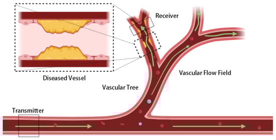
Figure 1.
Schematic of molecular transport in a cascaded vascular network. The vascular tree is modeled as communication sub-channels connecting a transmitter and receiver. Green arrows indicate blood flow and molecular propagation direction, while dashed rectangles mark the transmitter, receiver, and magnified diseased vessel. The yellow region represents atherosclerotic plaque causing vascular stenosis and altering local flow dynamics. The bloodstream shows cellular components (red) and macromolecular particulate components (blue, purple) to depict the actual molecular transport environment. Localized constrictions reshape the flow field and molecular transport, affecting signal delay and attenuation across the network.
In MC modeling, blood flow characteristics significantly influence signal transport. Under ideal Newtonian fluid conditions, the velocity profile follows classical Poiseuille flow, with axial velocity in a cylindrical pipe forming a parabolic distribution peaking at the center [25]. However, real blood flow is governed not only by plasma viscosity but also by the distribution of suspended particles such as red blood cells and platelets, often manifesting a “plug flow effect.” This phenomenon involves marked cell aggregation near the lumen center, leading to a flattened velocity profile (see Figure 2). It becomes more pronounced with decreasing vessel radius and shear rate, violating the Newtonian fluid assumption [26,27,28].
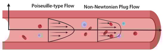
Figure 2.
Comparison of Poiseuille-type flow and non-Newtonian plug flow in blood vessels. In the image, red represents blood cells, blue and purple denote macromolecular substances in blood, and arrows indicate the direction of flow. For Poiseuille-type flow (approximating Newtonian fluid behavior), the velocity follows a parabolic distribution, with the maximum value at the vessel centerline. In contrast, real blood exhibits shear-thinning behavior due to the interaction between suspended blood cells and macromolecular substances in blood. This behavior leads to a flatter "plug-like" velocity profile, which becomes more pronounced in smaller vessels or stenosed regions where shear rates are relatively low.
Studies [29,30] show that blood behaves nearly like a Newtonian fluid in large arteries (diameter > 0.3 mm) but exhibits pronounced non-Newtonian characteristics in small vessels or stenosed regions due to low shear rates and cell aggregation. Accordingly, this study models blood as a non-Newtonian fluid. Among rheological models, the power-law form is chosen over the Casson or Cross models [31,32] for its simplicity, clear physical meaning, and suitability for deriving closed-form axisymmetric velocity distributions for arterial MC channels [33].
In the power-law model, the relationship between shear stress and shear rate is given by
where K is the consistency coefficient and n is the power-law index. This model is widely applicable to biological fluids, such as blood and saliva, that exhibit complex rheological behavior.
To simulate the branched human vascular structure, a tree-like network model is constructed (Figure 3), consisting of multiple cascaded pipe segments with nodes representing bifurcations. Within this cascade, each vessel segment is treated as an independent cylindrical channel characterized by length , radius , a fluid viscosity coefficient, and rheological behavior. Its time domain impulse response function describes the probability density of a messenger molecule released at time being received at time t, incorporating influences from blood flow velocity, diffusion, and vessel structure.
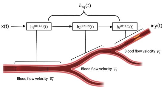
Figure 3.
Vascular modeling framework based on MC. The branched vessel network is represented as a cascade of cylindrical sub-channels, each characterized by its own length, radius, and flow velocity. The time domain impulse response of each segment captures the effects of convection, diffusion, and vessel geometry. The overall system response, , is obtained by convolving the sub-channel responses, thereby linking local vascular dynamics to signal propagation across the entire network.
For a complete pathway formed by sequentially connecting segments, the signal undergoes the response processes of each sub-channel. Using to denote , the overall system CIR, , is the time domain convolution of the sub-channel responses
Before proceeding with the derivation of healthy and stenosed vessel models, we first clarify the assumptions and scope underlying the proposed vascular channel formulation.
2.1. Assumptions and Scope
The formulation of MC channels in biological environments generally relies on a set of simplifying assumptions to balance analytical tractability with physiological realism. Without such abstractions, closed-form solutions are often intractable, and key insights into channel behavior may be obscured by numerical complexity. In line with this established practice, the vascular channel model developed here adopts assumptions that emphasize the principal hemodynamic and transport features while maintaining mathematical clarity.
Specifically, blood is modeled as a non-Newtonian fluid following a power-law rheology to capture shear-thinning effects observed in micro- and meso-scale vessels. Stenoses are idealized as symmetric, bell-shaped geometries, offering a physiologically interpretable yet mathematically convenient representation of luminal narrowing. Vessel walls are treated as rigid, and flow is assumed to be steady, neglecting pulsatile variations and wall elasticity. In addition, hematocrit is considered uniform, so that variations in red blood cell concentration and their effect on viscosity are not explicitly modeled.
These assumptions enable the derivation of closed-form channel impulse responses and facilitate systematic analysis of adsorption–desorption kinetics within cascaded vascular segments. At the same time, they delimit the scope of the model and may lead to deviations in scenarios involving asymmetric stenoses, pulsatile hemodynamics, elastic wall deformation, or heterogeneous hematocrit distributions. Addressing these factors constitutes an important avenue for future refinement and validation.
2.2. Channel Modeling of Healthy Vascular Structure
2.2.1. Non-Newtonian Fluid Modeling and Velocity Profile Derivation
Consider an incompressible power-law fluid driven by a constant axial pressure gradient; ( is the pressure gradient magnitude. Under fully developed flow conditions, the axial velocity component varies only radially (), and radial/tangential velocity components are zero (). Combining axisymmetry (), fluid dynamics are described by the power-law constitutive equation
where is the shear stress, K (Pa·sn) is the consistency coefficient, and n is the power-law index ( characterizes blood shear-thinning behavior).
The axial momentum equation in cylindrical coordinates simplifies to
Integrating Equation (4) and applying the bounded shear stress condition at the pipe center (, finite) yields the shear stress distribution
Combining the constitutive Equation (3) and stress solution (5), and considering the negative velocity gradient in pipe flow (), gives
Rearranging Equation (6) provides the explicit velocity gradient
Integrating Equation (7) from r to R and applying the no-slip boundary condition at the wall () yields the analytical velocity profile:
The profile shape depends on n. For (Newtonian fluid), it is parabolic. For , the center velocity flattens, forming a distinct “plug flow.” For (shear-thickening), the velocity gradient increases, and overall velocity decreases.
Volume flow rate Q is calculated by integrating the velocity profile
Average velocity is defined as
2.2.2. Impulse Channel Response Derivation
In healthy vessel molecular transport, convection diffusion forms the theoretical basis. The spatiotemporal evolution of MC in a straight cylindrical vessel of length L follows the partial differential equation
where is the segment average velocity (from Equation (10)) and D is the diffusion coefficient.
Given the initial condition and developed flow boundary conditions, Equation (11) admits the analytical solution
To model the physiological loss of messenger molecules permeating the vessel wall into surrounding tissue, an exponential decay factor is introduced, yielding the modified CIR
where is the physiological signal decay rate constant. A larger signifies shorter messenger molecule retention within the vessel. This term captures concentration decay due to healthy vessel wall permeability without altering the core equation structure.
2.3. Channel Modeling of Stenosed Vascular Structure
2.3.1. Geometric Parameterization and Hemodynamic Basis
Accurate flow field modeling in stenosed vessels relies on appropriate stenosis geometry. Studies show that real arterial stenoses are often symmetric or near-symmetric and can be described by bell-shaped functions, which capture velocity, pressure, and shear stress variations effectively [34,35,36]. The vessel is modeled as an inlet healthy segment, a bell-shaped contraction, a bell-shaped recovery, and a healthy outlet segment. The contraction and recovery are axially symmetric, each of length , while the healthy segments each span , giving a total stenosed length of (Figure 4).
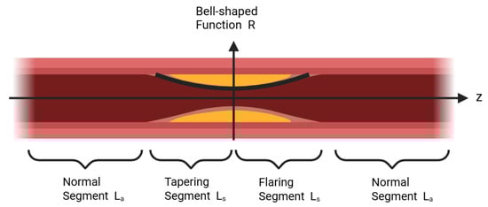
Figure 4.
Vascular modeling scheme for a stenosed segment. In the image, yellow areas depict stenotic lesions, while dark red parts represent healthy vascular tissue. The vessel is divided into a healthy inlet region, a bell - shaped contraction, a bell - shaped recovery, and a healthy outlet region. Each contraction and recovery segment has a length , and the adjacent healthy segments each have a length , resulting in a total stenosed length of . The bell - shaped radius function captures the symmetric narrowing and recovery of the lumen, offering a physiologically meaningful foundation for analyzing flow velocity, pressure, and shear stress in stenosed vessels.
The radius function in the axial coordinate z is defined as
where is the healthy segment radius, a is the ratio of maximum stenosis depth to (), and controls stenosis concentration. For and , .
Under constant pressure difference , the power-law fluid satisfies continuity
where is the healthy segment volumetric flow rate.
The local flow rate in the stenosis is
The axial average velocity is defined as
Substituting yields
To provide a more intuitive visualization of blood flow velocity and MC distributions, we performed numerical simulations in COMSOL Multiphysics 6.2 using the established fluid dynamics model. Figure 5 presents velocity distributions for different stenosis depths, and Figure 6 shows the corresponding spatial MC distributions within the vessel. These results offer critical physical insights that underpin the subsequent calculation of the CIR and analysis of delay characteristics.
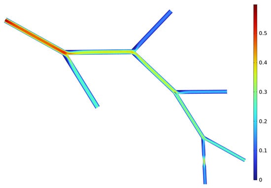
Figure 5.
Velocity distribution in the simulated vascular model. The color map shows local blood flow velocity across the branched network, with higher velocities near constricted regions and lower velocities in wider branches. These results illustrate how stenosis alters the hemodynamic environment and provides the basis for subsequent analysis of molecular transport.
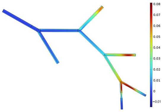
Figure 6.
Concentration distribution of messenger molecules during flow (, ). The spatial distribution highlights regions of molecular accumulation and dispersion along the vascular tree, reflecting the combined effects of convection, diffusion, and stenosis-induced flow disturbance. This visualization offers key physical insights for calculating channel impulse responses (CIRs) and delay characteristics.
2.3.2. Derivation of Impulse Channel Response
Under atherosclerotic conditions, stenosed regions often show vessel wall damage, endothelial dysfunction, and abnormal receptor expression, which enhance wall adsorption of messenger molecules and induce reactive binding during propagation [32,37]. This is modeled by incorporating adsorption/dissociation kinetics into the stenosed segment, where molecules bind to endothelial receptors and later dissociate at rate into the free state. The process, governed by the adsorption rate and dissociation rate , introduces the bound concentration , which couples with the convection–diffusion equation to yield:
Initial conditions are set as a Dirac pulse input; and . To eliminate convection, we apply the Galilean transformation , which gives the derivative relations and . Substituting these into Equation (20) simplifies it to
Equation (21) remains unchanged. Applying the Laplace transform with respect to t yields the governing equations
the governing equations become
Solving Equation (25)
Substituting into Equation (24)
Simplifying the coefficient
Equation (28) is a 1D Helmholtz equation. Its Green’s function solution is
where . The time domain solution is obtained via the inverse Laplace transform
By fixing the observation at position x, the corresponding impulse response can be written as follows:
Focusing on messenger molecules propagating from release to reception points, and fixing the propagation distance at the receiver position , the impulse response is formalized as a function of time
The adsorbed phase concentration is
It is noted that the unilateral Laplace transform inherently enforces causality, i.e., for . Moreover, the CIR in Equation (32) is concentration-based rather than a first-passage probability density; its time integral is finite only under decay terms such as or , which provide the condition for normalization.
For completeness, we consider the limiting behavior of Equation (32) under two extreme kinetic regimes.
- (A)
- (no adsorption).
- (B)
- (instantaneous desorption).In this regime the bound phase approaches the quasi-steady state , so the net exchange tends to zero. Physically, molecules attach but are immediately released, producing no effective retention. As a result, Equation (32) again reduces to
Both limits converge to the free convection–diffusion response, with an additional exponential factor included when physiological decay is present in healthy vessels.
2.3.3. Flow Resistance and Shear Stress
To elucidate how stenosed structures modulate flow resistance and shear stress, dimensionless expressions are analytically derived using the bell-shaped radius model.
Starting from the power-law fluid constitutive relation and Equation (17)
Shear stress relates non-linearly to the velocity gradient. Its expression is
Under a fixed pressure drop
This result shows that shear stress is proportional to the radius function along z. Maximum shear stress occurs at the throat , corresponding to the minimum radius :
here, we define as the peak wall shear stress at the throat (). Thus, the throat shear stress peak increases linearly with stenosis ratio a. As stenosis worsens (), rises sharply, potentially inducing endothelial stress-related changes in molecular attachment, endothelial dysfunction, and physiological damage.
To quantify the increase in overall flow resistance due to stenosis, resistance per unit pressure difference is defined as
The dimensionless resistance (normalized by healthy segment resistance ) is
This expression, solvable via numerical integration, reveals significant sensitivity of impedance to the stenosis ratio a, distribution range b, and power-law index n.
3. Biodistribution Estimation
Biodistribution analysis aims to elucidate the spatial distribution and enrichment of messenger molecules within the vascular system. It encompasses transport processes and interactions, including permeation into surrounding tissues or reactions with blood components. This section employs two key MC performance parameters—path delay and path loss—to evaluate distribution characteristics and transmission efficiency.
3.1. Channel Delay Analysis at Receiver
Channel delay () denotes either the mean transit time or peak response time required for information molecules to propagate from the release point to the reception point. Vascular structures, particularly stenoses, significantly influence fluid velocity, diffusion characteristics, and molecular reaction kinetics, establishing delay as a vital indicator of vascular pathology.
3.1.1. Healthy Vessel Delay
In healthy vessels, molecules propagate axially under laminar flow, influenced by diffusion and physiological decay (Equation (13)). Peak time satisfies as follows:
Assuming weak diffusion () and retaining dominant terms yields
where the first term represents the convection-dominated propagation time, the second term corresponds to the diffusion-induced advancement, and the third term denotes the concentration peak advancement resulting from physiological decay.
3.1.2. Stenosed Vessel Delay
In stenosed vessels caused by pathologies such as atherosclerosis, propagation is influenced by both altered blood flow velocity and adsorption–desorption at the vessel wall. This surface reaction causes molecule retention, so delay is no longer dominated solely by transport. Using a reversible adsorption kinetics description, where denotes the bound molecule concentration, characteristic time scale analysis indicates that delay comprises
The first term is the effective transport time under stenosis, and the second term is the average residence time on the vessel wall. Together, they constitute the total signal transmission delay in stenosed vessels. This theoretical trend is consistent with in vivo observations; for example, Takeuchi et al. (2023) showed that arterial transit time (ATT) is significantly prolonged in patients with carotid artery stenosis, reflecting delayed passage of blood through narrowed vessels [38]. Engelhard et al. (2022) found reduced velocity and disturbed flow downstream of aortoiliac stenoses using high-frame-rate contrast-enhanced ultrasound velocimetry, indicating slower propagation of flow in stenosed vascular paths [39]. Carrozzi et al. (2025) reviewed multiple ASL MRI studies showing consistent pre-operative perfusion deficits in brain regions supplied by stenosed carotid arteries, suggesting impaired downstream supply which aligns with the increased delay in transmission in the theoretical model [40].
3.2. Path Loss Analysis
Consider an m-layer vascular binary tree structure, where each layer represents a branch level or vessel segment. Assume layer j is stenosed and that the others are healthy. Signals propagate sequentially from the inlet to the end receiver. The system-level time varying CIR is defined as
where is the healthy segment CIR for layer i, and is the stenosed segment response.
Path loss is defined as the logarithmic attenuation of the fraction of molecules that successfully reach the receiver under unit concentration input
where is the effective transmission probability along the path. For calibration, correspond to , respectively.
For analytical modeling, introduce the transmission retention rate for each segment
Assuming probabilistic independence, the total transmission probability is
Thus, path loss is
The healthy vessel loss factor is
The stenosed vessel loss factor is
where is the power-law fluid coefficient.
The closed-form path loss is
These expressions show that path loss depends on the cumulative attenuation of healthy segments and the stenosed segment loss factor . increases with path length and attenuation coefficient , while is determined by stenosis severity a and adsorption–desorption kinetics . Greater a or raises path loss, whereas higher reduces it, establishing a quantitative link between vascular morphology, molecular interactions, and communication efficiency in diseased vessels.
It should be emphasized that in deriving Equation (48), the product form arises from the separability of convolution integrals under a linear and time-invariant assumption, rather than from a probabilistic independence postulate. In practical scenarios, however, molecular receivers operate with a finite detection window per symbol, and molecules are released at intervals . When the equivalent channel response exhibits long temporal tails, contributions from adjacent symbols overlap within the same window, resulting in inter-symbol interference (ISI). To evaluate this effect, convolution-based simulations were conducted to compare the product prediction with the detectable fraction within . The results indicate that the product approximation remains accurate when exceeds, by four to six times, the RMS delay spread of and adsorption is weak (), whereas in fast-signaling regimes with strong adsorption the deviation becomes significant. Representative validation results, including the relative deviation and the ISI index as functions of , are shown in Figure 7 and Figure 8, highlighting both the validity range and the inherent limitations of the product formulation.
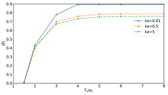
Figure 7.
Convolution-based validation: relative deviation between product approximation and convolution results as a function of normalized symbol period for different adsorption rates . The deviation decreases when is sufficiently large, confirming the validity range of the product formulation.
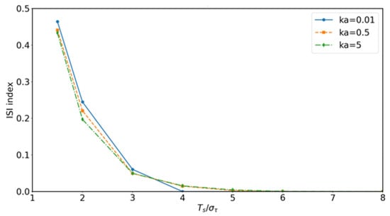
Figure 8.
Convolution-based validation: inter-symbol interference (ISI) index versus a normalized symbol period for different adsorption rates . Strong adsorption and short yield higher ISI, while sufficiently long mitigates symbol overlap, demonstrating the limits of the product-based approximation.
4. Atherosclerosis Delay Localization Method
The delay localization method estimates the location of atherosclerosis by analyzing messenger molecule propagation delays across vascular structures. Within the MC framework, peak response time (tp) is used as the delay metric, establishing a functional mapping between stenosis parameters and signal characteristics. The process involves (1) the forward modeling of stenosis at discrete positions, simulating vessel variants, and recording downstream ; (2) inverse matching of the measured arrival times to the simulation results to infer lesion location, achieving a high resolution and scalability.
4.1. Forward Problem: Peak Time Extraction
Previous studies have explored various metrics for vascular anomaly detection in MC. For instance, Sun et al. (2022) adopted an arrival probability-based indicator, measuring the fraction of nanoparticles reaching the outlet under stenosis [11]; centroid-based measures have been applied to characterize mean transport delay in particulate drug-delivery systems [41]; and statistical bounds such as the Cramér–Rao bound (CRB) have been derived for source localization problems [42]. However, arrival probability and centroid metrics are sensitive to long diffusive or adsorptive tails, while CRB provides only a theoretical performance limit rather than a directly measurable quantity. In contrast, the peak response time used in this study is directly observable from , is robust against tail effects, and is computationally efficient under adsorption–desorption kinetics [43]. Therefore, although multiple alternatives exist, peak response time offers the most intuitive, robust, and practically computable metric for vascular stenosis detection, as summarized in Table 1.

Table 1.
Comparison of delay-related metrics in MC.
For an m-layer binary tree with stenosis at layer j and severity ,
is highly sensitive to j and s due to flow reduction, adsorption enhancement, and diffusion changes. Simulating over multiple pairs forms a forward database for inverse problem localization.
4.2. Inverse Problem: Atherosclerosis Detection
The forward problem constructs vessel models characterized by stenosis at distinct layers and severities , recording the corresponding receiver peak time for each parameter combination. The inverse problem aims to infer the stenosed layer j and severity s from an experimentally observed peak time .
Assuming Gaussian timing noise, the observation error is modeled as , where is the standard deviation of peak time measurement uncertainty. The corresponding likelihood function is
where
Here is no longer an empirical coefficient but is directly determined by the timing noise variance. A larger corresponds to higher measurement uncertainty and thus a smaller , leading to a smoother similarity surface. Conversely, a smaller yields sharper discrimination between different candidates.
To obtain a normalized posterior confidence, we further compute
where denotes the prior distribution of stenosis parameters, chosen to be uniform in this work. The pair maximizing is identified as the most probable stenosis location and severity.
5. Discussion
Figure 9 illustrates how the interplay between healthy segment length and stenosed segment length influences the average flow velocity . While a longer slightly reduces , the effect of is substantially more pronounced; extending the stenosed region from to mm produces a marked velocity drop, reflecting the cumulative resistance imposed by prolonged luminal narrowing. Pathophysiologically, this result is consistent with the clinical observation that extended stenotic lesions aggravate flow restriction and increase the risk of downstream hypoperfusion. From a diagnostic perspective, this emphasizes that both stenosis depth and longitudinal extent should be considered when assessing disease severity, since longer lesions may impair perfusion even at moderate narrowing. The shaded uncertainty bands (mean ± 1 SD) arising from variability in the power-law index () confirm that these hemodynamic trends remain robust against inter-individual differences in blood rheology, thereby supporting the translational relevance of the model predictions.
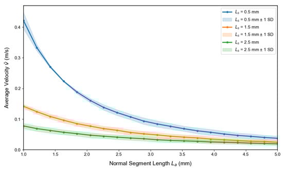
Figure 9.
Influence of stenosed segment length and healthy segment length on the average velocity . Increasing leads to a moderate reduction in across all stenosis configurations, while longer stenosed segments ( mm) cause a pronounced velocity drop compared to shorter ones ( and mm). The shaded bands (mean ± 1 SD) represent variability due to the power-law index (), confirming the robustness of these trends under physiological uncertainty.
Figure 10 depicts the effect of stenosis depth a and steepness b on the average velocity for a vessel of fixed length cm with . The results demonstrate that decreases sharply with increasing a, establishing stenosis depth as the dominant determinant of flow reduction. In contrast, variations in b exert only a modest influence, producing minor changes in velocity compared with the effect of a. From a hemodynamic perspective, this indicates that luminal narrowing primarily governs resistance to blood flow, while the geometric steepness of the lesion plays a secondary role. Clinically, this highlights the importance of lesion severity in determining downstream perfusion deficits, consistent with observations that deeper stenoses pose higher risks of ischemia even when their axial extent is limited. The translucent uncertainty envelopes (mean ± SD from Monte Carlo simulations, ) confirm that these relationships are robust under physiological variability in blood rheology and vessel properties, supporting the translational relevance of the model predictions.
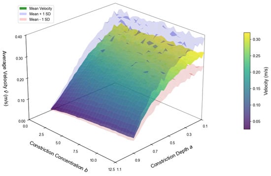
Figure 10.
Average velocity versus stenosis depth a and steepness b. The surface represents mean values, and translucent envelopes indicate mean ± SD obtained from Monte Carlo simulations () accounting for parameter variability.
Figure 11 presents the channel impulse responses (CIRs) for healthy and stenosed vessels under varying adsorption–desorption kinetics. In the analytical results (left), the healthy vessel produces a tall and narrow peak, reflecting efficient signal transmission. In contrast, increasing attenuates the peak, while larger elongates the decay phase, producing extended molecular retention within the stenosed region. This tail broadening implies stronger temporal dispersion of molecular signals, which in physiological terms corresponds to prolonged tracer residence and delayed clearance in diseased vessels. The Monte Carlo simulations (right) reproduce these features with high fidelity, confirming that the analytical formulation reliably captures both the attenuation and dispersion mechanisms that characterize stenosed vascular communication channels.
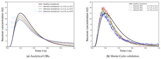
Figure 11.
Channel impulse responses (CIRs) for healthy and stenosed vessels under varying adsorption parameters (, ). (a) Analytical results show that the healthy vessel exhibits the highest and sharpest peak, whereas increasing reduces peak amplitude and larger extends the response tail, leading to stronger inter-symbol interference (ISI). (b) Monte Carlo particle-based validation demonstrates concentration–time curves that closely follow the analytical trends, confirming both the accuracy and robustness of the derived model.
Figure 12 and Figure 13 illustrate the effects of stenosis depth and constriction steepness b on wall shear stress distributions . An increase in markedly elevates the peak shear stress at the throat, indicating a stronger hemodynamic burden as the vessel lumen narrows. By contrast, increasing b sharpens and narrows the stress profile, concentrating the load over a smaller axial region. From a pathophysiological perspective, both deeper and sharper stenoses amplify local mechanical forces on the endothelium, conditions known to promote endothelial dysfunction, inflammatory activation, and accelerated plaque progression. The shaded regions denote mean ± SD from Monte Carlo samples accounting for physiological variability, confirming that these trends are robust against individual differences in vascular parameters. Clinically, these results underscore that not only stenosis severity but also its morphological shape critically determines the risk of lesion destabilization and adverse vascular events.
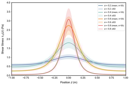
Figure 12.
Influence of stenosis depth on wall shear stress distribution . Curves show mean values, with shaded bands denoting mean ± SD from Monte Carlo samples.
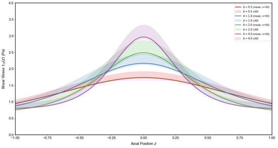
Figure 13.
Influence of constriction steepness b on wall shear stress distribution . Mean profiles with shaded mean ± SD envelopes illustrate the narrowing and amplification of the stress peak with increasing b.
Figure 14 and Figure 15 demonstrate how adsorption–desorption kinetics interact with flow velocity to shape MC performance. As the adsorption-to-desorption rate ratio increases, path delay rises steeply, indicating prolonged molecular residence at the vessel wall. This effect is particularly pronounced under low-flow conditions, where convection is insufficient to offset adsorption. In parallel, higher elevates path loss by reducing the proportion of molecules reaching the receiver, again with the strongest impact observed at slow velocities. Pathophysiologically, these findings reflect how endothelial binding and delayed release under stenotic or hypoperfused states can both slow and weaken molecular signals. Clinically, they highlight that low-flow environments exacerbate diagnostic uncertainty, underscoring the need for system designs that adapt to variable hemodynamic conditions.
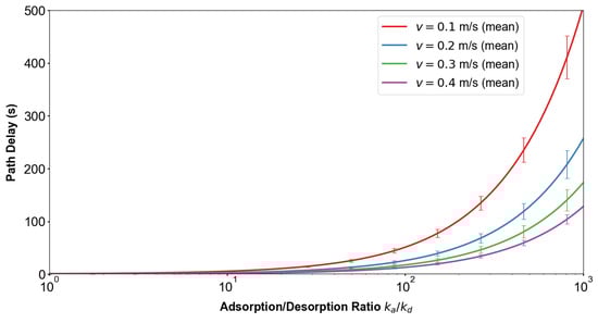
Figure 14.
Influence of adsorption rate and flow velocity on delay time. Increasing the adsorption-to-desorption rate ratio markedly prolongs path delay, with the effect being stronger at lower velocities. Error bars (mean ± 1 SD) indicate variability due to stochastic fluctuations in molecular propagation, confirming that adsorption significantly slows signal transmission under low-flow conditions.
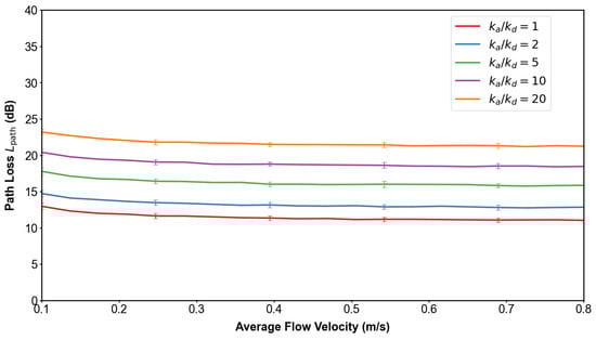
Figure 15.
Influence of adsorption rate and flow velocity on path loss. Higher values increase molecular absorption at the vessel wall, thereby reducing the fraction of molecules reaching the receiver and elevating path loss. The trend is most pronounced under slow flow, indicating that adsorption dominates over convection when velocity is low.
6. Simulation Validation of Vascular Stenosis Detection Based on Delay Inversion
To validate the peak response time-based inversion method for vascular stenosis detection, we employed the COMSOL model described in Section 2. The two-dimensional axisymmetric model (total length cm) comprised a first-level vessel segment of 5 cm, with subsequent levels shortened by cm, and an initial radius of 2 mm decreasing by mm per level. A stenotic segment (at the j-th level) was individually introduced with severity . Laminar flow physics solved the velocity field under a constant inlet pressure drop Pa (outlet at atmospheric pressure), with blood density 1060 kg/m3 and viscosity Pa·s. The Dilute Species Transport module simulated messenger molecule convection/diffusion ( m2/s). In each run, a unit pulse was released at the inlet, and the outlet concentration–time curve at the terminal vessel level was recorded as the received signal.
For all combinations of stenosis location () and severity (), the signal peak time was extracted. These values constitute the standard response time matrix presented in Table 2.
Table 2.
Messenger molecule peak time for atherosclerosis at different locations (unit: s).
In the inverse problem, an unknown stenosis model produced a measured peak concentration time of s. The similarity metric was computed for each combination using Equation (55). These similarity values were then projected onto a two-dimensional map representing the five-layer vessel structure (Figure 16). The region exhibiting the highest intensity corresponds to the most probable stenosis severity and location.
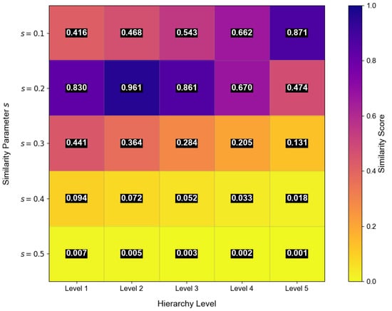
Figure 16.
Delay localization scan image for atherosclerosis using messenger molecules. The two-dimensional similarity map encodes stenosis severity s and vascular layer j, where higher intensity indicates a closer match between measured and modeled peak times. The highlighted region at corresponds to the most probable stenosis configuration, demonstrating the ability of the delay inversion framework to jointly estimate both lesion location and severity.
In addition to the COMSOL-based validation of the delay inversion method, we further investigated the identifiability of the model parameters by analyzing the local sensitivity of the peak time with respect to variations in stenosis depth a, kinetic rates and , average velocity , and vessel path length L. The relative sensitivity (elasticity) was quantified as
where denotes the i-th parameter in , is its baseline value, and is the corresponding peak time, evaluated around the baseline configuration .
Figure 17 summarizes the local sensitivity and identifiability of the delay inversion framework. Panel (a) shows that peak time is highly sensitive to stenosis depth a, confirming that temporal delays directly encode lesion severity. Panel (b) reveals a degeneracy between vessel length L and average velocity , indicating that distinct geometric flow configurations can yield similar arrival times; this highlights a potential source of ambiguity that in practice may require auxiliary measurements to resolve. Panel (c) demonstrates that adsorption and desorption kinetics (, ) jointly shape delay responses, reflecting the dual role of endothelial binding and release in prolonging molecular retention. Across all panels, the regression fits yield with statistically significant correlations (), and the shaded envelopes confirm that parameter identifiability remains stable even under measurement noise. Together, these findings indicate that the proposed inversion approach can robustly recover key physiological parameters from noisy data, providing a reliable basis for quantitative assessment of vascular lesions in clinically relevant conditions.
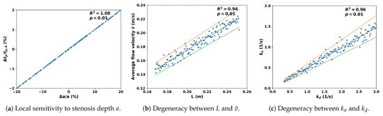
Figure 17.
Local sensitivity and identifiability analysis of the delay inversion approach. Scatter points denote 130 perturbed samples, dashed lines are regression fits, shaded bands indicate 95% confidence intervals, and dotted envelopes correspond to limits.
In addition to the local sensitivity analysis, we further evaluated the robustness of the proposed delay inversion framework under measurement noise. Specifically, Gaussian perturbations were added to the peak time observation as
where was normalized with respect to the median nearest neighbor spacing in the reference delay library. For each noise level, random samples were generated and repeated times to obtain mean accuracies and standard deviations. Classification was then performed using the same nearest neighbor rule as in (55).
Figure 18 evaluates the robustness of the delay inversion framework under Gaussian noise. Classification accuracy remains above 95% when and still exceeds 80% at , indicating that the method tolerates moderate measurement uncertainty. This robustness is clinically relevant because physiological data are inevitably affected by pulsatility, sensor artifacts, and biological variability. Figure 19 further shows confusion matrices under different noise levels, where diagonal dominance is largely preserved, confirming that stenosis location and severity remain identifiable in most cases. Nonetheless, performance degrades when noise becomes excessive, especially in finer severity distinctions, underscoring that practical deployment will require careful calibration of sensing accuracy or multi-modal integration. Overall, these results support the diagnostic feasibility of the framework under realistic uncertainty while acknowledging its sensitivity to extreme noise conditions.
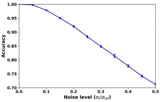
Figure 18.
Robustness of the delay inversion framework under Gaussian noise. The curve shows classification accuracy (mean ± std over 20 repeats) versus normalized noise level . Accuracy remains above when , and still exceeds at .
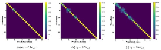
Figure 19.
Confusion matrices aggregated over 20 Monte Carlo repeats at three representative noise levels. Rows correspond to the true classes (five stenosis severities × 5 vascular levels), while columns denote the predicted classes. At low noise (), predictions remain highly accurate with clear diagonal dominance. As noise increases ( and ), off-diagonal entries gradually emerge, yet the majority of cases are still correctly classified, confirming the robustness of the delay inversion framework under realistic uncertainty.
Based on the Gaussian likelihood similarity function defined in Equation (55), we evaluated the ability of the proposed framework to resolve small differences in stenosis severity under different noise conditions. For each vascular level , the five anchor severities were used as reference points (see Table 2). Pairs of hypotheses versus were compared, and the decision was made by maximum likelihood. Classification accuracy was estimated by Monte Carlo simulations with trials for each condition. Three severity gaps were examined under noise levels .
Figure 20 evaluates the resolution limits of stenosis severity classification under noise. While larger severity gaps () are almost perfectly distinguished and moderate gaps () remain reliably separable above 95% for s, very small gaps () are more sensitive to noise and fall below this threshold at higher . These findings indicate that the framework can robustly resolve clinically relevant categories such as mild versus moderate stenosis, but its ability to detect extremely subtle changes is limited, especially under noisy or proximal conditions. Clinically, this suggests practical feasibility for routine assessments while highlighting the need for complementary modalities or higher-fidelity sensing when early, borderline lesions are of concern.
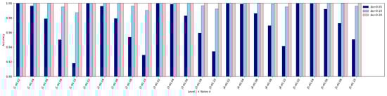
Figure 20.
Resolution limit analysis of stenosis severity classification. Bars represent classification accuracy for three severity gaps , , and across all vascular levels and noise conditions. Larger severity differences () remain almost perfectly distinguishable under all tested noise levels, while moderate gaps () maintain accuracy above for most cases when s. In contrast, very small differences () are more sensitive to noise, with accuracy dropping below at s, particularly in proximal vessel levels. These findings confirm that the framework can robustly resolve stenosis severity differences down to under practical noise conditions.
As a further validation, we compared the proposed peak response time inversion framework with several representative methods for vascular stenosis detection and functional assessment reported in the recent literature. As summarized in Table 3, existing imaging and deep learning approaches generally achieve moderate-to-high diagnostic accuracy. For example, ASL-MRI studies show only moderate correlation with PET-CBF (R2 or –0.75), while CT-based functional assessment reaches higher accuracy (∼96%) but relies on high-quality images and complex algorithmic deployment. Deep learning models for angiography also report excellent F1-scores but require extensive labeled datasets. In contrast, our method achieves localization accuracy under low-noise conditions and remains even with significant noise, with the additional ability to resolve 10% stenosis differences. These results indicate that the proposed framework is highly competitive with state-of-the-art methods and demonstrates superior robustness and a fine-grained resolution, despite being validated solely through simulations.
Table 3.
Comparison of recent methods for vascular stenosis detection with the proposed approach.
7. Experimental Platform for Fluorescence-Based Detection
In our previous work [48], we developed a fluorescence-excitation MC platform to illustrate how molecular transport signals can be generated and detected in practice. Although built independently of the present study, this testbed establishes a tangible link between the theoretical framework proposed here and its biomedical applicability to stenosis detection.
The platform employs Rhodamine B as the messenger molecule, injected into a micro-tube channel by a solenoid valve under a background flow generated by a peristaltic pump. At the receiver, a 525 nm LED excites the dye, and an AS-7262 spectral sensor captures the resulting fluorescence near 580 nm. In this way, changes in peak molecular concentration are converted into optical intensity signals, making it possible to observe peak response times that correspond to the inversion method introduced in this paper. The overall setup, including transmitter, channel, and receiver components, is shown in Figure 21.
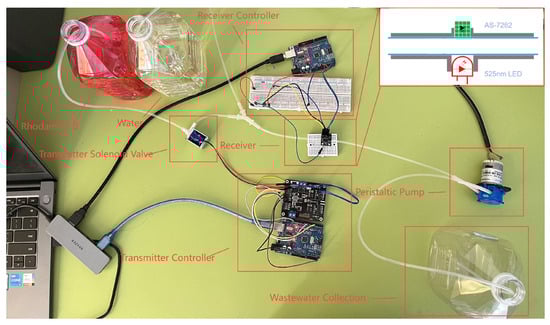
Figure 21.
Experimental test bench for fluorescence-based MC. The setup integrates a transmitter, channel, and receiver: Rhodamine B dye is injected into a micro-tube channel by a solenoid valve under background flow generated by a peristaltic pump. At the receiver, a 525 nm LED excites the dye, and an AS-7262 spectral sensor records fluorescence near 580 nm. This configuration enables real-time measurement of peak molecular concentrations as optical intensity signals, thereby linking the proposed theoretical inversion framework with a tangible biomedical testbed for stenosis detection.
Experimental trials further demonstrate the feasibility of reliable symbol transmission. As shown in Figure 22, the concentration waveform of a 50-bit sequence exhibits clearly distinguishable peaks, and the corresponding response times can be directly identified. This confirms that the central concept of this work—stenosis-induced peak delay—can be physically translated into measurable optical signals.
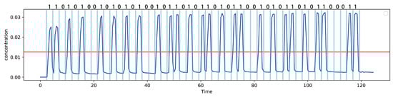
Figure 22.
Measured Measured concentration waveform for the transmission of a 50-bit sequence. The blue line represents the concentration of messenger molecules received at the receiver end. The red line is a threshold line, whose value is related to the peaks of the first and second signals. If the concentration exceeds this value, the received signal is determined to be 1; otherwise, it is 0. Distinct peaks corresponding to individual bits are clearly observed, demonstrating that the spectral sensor can reliably detect symbol transitions. The temporal positions of the peaks directly encode the response times, confirming that stenosis-induced peak delays can be translated into measurable optical signals for practical MC experiments.
It should be noted that Rhodamine B, while convenient for proof of concept due to its strong fluorescence and stability, has certain toxicity and is not suitable for direct biomedical applications. Moreover, in this work we modeled adsorption–desorption kinetics with parameters , which cannot be fully replicated by Rhodamine B in aqueous solution. Future extensions of the platform will therefore explore more biologically relevant messengers, such as blood-derived fluids (e.g., pig blood or plasma components), to better capture adsorption–desorption effects at vascular interfaces and to ensure safe in vitro and in vivo validation. This direction will allow for the experimental setup to more closely reflect the conditions assumed in the theoretical model presented in this study.
8. Conclusions
This study develops a cascaded MC channel model for early detection of vascular stenosis, combining power-law non-Newtonian fluid dynamics, bell-shaped constriction geometry, and adsorption–desorption kinetics. Closed-form impulse responses were derived, and path delay and path loss were introduced as generalizable performance metrics for multi-segment vascular networks. Numerical and simulation analyses demonstrated that both stenosis depth and adsorption–desorption dynamics substantially influence flow resistance, wall shear stress, and molecular signal propagation.
A delay inversion method based on peak response time was proposed to jointly estimate stenosis location and severity. Simulation studies confirmed a high spatial resolution and tolerance to measurement noise, supporting its potential integration into IoBNT and wireless sensor network architectures. The robustness observed in this work should, however, be interpreted within the scope of the tested conditions, and additional evaluations under Newtonian flow, variable pressure gradients, and other ablation scenarios will be essential for broader validation.
From a biomedical perspective, the framework provides a pathway toward non-invasive vascular health monitoring. Its primary utility may lie in early screening applications, where continuous and minimally intrusive assessment is critical. Future in vitro studies with blood analog fluids and vessel-mimicking channels, followed by in vivo validation, will be necessary to establish translational feasibility. Integration with wearable or implantable biosensors could ultimately enable adaptive feedback systems for preventive cardiovascular care.
Several limitations should be acknowledged. The present model assumes symmetric stenosis, steady flow, and homogeneous hematocrit, while real vascular environments involve pulsatility, elasticity, and heterogeneity. Extending the framework to asymmetric or multi-lesion geometries, incorporating dynamic hemodynamics, and conducting clinical-scale experiments will be important directions. Overall, the work establishes an analytically tractable and physiologically grounded framework for MC in stenosed vessels, providing both theoretical foundation and technical pathways toward personalized, IoT-enabled cardiovascular monitoring.
Author Contributions
Conceptualization, Z.S., P.Z., and X.W.; methodology, Z.S., P.Z. and X.W.; software, Z.S.; investigation, Z.S. and P.Z.; writing—original draft preparation, Z.S. and P.Z.; writing—review and editing, P.Z., X.W. and P.L.; supervision, P.Z., X.W. and P.L.; funding acquisition, X.W. and P.L. All authors have read and agreed to the published version of the manuscript.
Funding
This work was supported by the Tianchi Elite Youth Doctoral Program (CZ002717, CZ002701, CZ002707) and the High-Level Talent Research Initiative Program of Shihezi University (RCZK202322).
Institutional Review Board Statement
Not applicable.
Informed Consent Statement
Not applicable, since this study did not involve human participants or animals.
Data Availability Statement
The simulation parameters and COMSOL 6.2 files used to support the findings of this study are available from the corresponding author upon reasonable request.
Conflicts of Interest
The authors declare no conflicts of interest.
Abbreviations
The following abbreviations are used in this manuscript:
| MC | Molecular Communication |
| IoBNT | Internet of Bio-Nano Things |
References
- Libby, P.; Buring, J.E.; Badimon, L.; Hansson, G.K.; Deanfield, J.; Bittencourt, M.S.; Tokgözoğlu, L.; Lewis, E.F. Atherosclerosis. Nat. Rev. Dis. Prim. 2019, 5, 56. [Google Scholar] [CrossRef]
- Virani, S.S.; Alonso, A.; Aparicio, H.J.; Benjamin, E.J.; Bittencourt, M.S.; Callaway, C.W.; Carson, A.P.; Chamberlain, A.M.; Cheng, S.; Delling, F.N.; et al. Heart Disease and Stroke Statistics—2021 Update: A Report From the American Heart Association. Circulation 2021, 143, e254–e743. [Google Scholar] [CrossRef]
- Falk, E. Pathogenesis of atherosclerosis. J. Am. Coll. Cardiol. 2006, 47, C7–C12. [Google Scholar] [CrossRef]
- Budoff, M.J.; Dowe, D.; Jollis, J.G.; Gitter, M.; Sutherland, J.; Halamert, E.; Scherer, M.; Bellinger, R.; Martin, A.; Benton, R.; et al. Diagnostic performance of 64-multidetector row coronary computed tomographic angiography for evaluation of coronary artery stenosis in individuals without known coronary artery disease: Results from the prospective multicenter ACCURACY trial. J. Am. Coll. Cardiol. 2008, 52, 1724–1732. [Google Scholar] [CrossRef]
- Okamura, T.; Tsukamoto, K.; Arai, H.; Fujioka, Y.; Ishigaki, Y.; Koba, S.; Ohmura, H.; Shoji, T.; Yokote, K.; Yoshida, H.; et al. Japan Atherosclerosis Society (JAS) Guidelines for Prevention of Atherosclerotic Cardiovascular Diseases 2022. J. Atheroscler. Thromb. 2024, 31, 641–853. [Google Scholar] [CrossRef] [PubMed]
- Farsad, N.; Yilmaz, H.B.; Eckford, A.; Chae, C.-B.; Guo, W. A comprehensive survey of recent advancements in molecular communication. IEEE Commun. Surv. Tutorials 2016, 18, 1887–1919. [Google Scholar] [CrossRef]
- Felicetti, L.; Femminella, M.; Reali, G.; Liò, P. Applications of molecular communications to medicine: A survey. Nano Commun. Netw. 2016, 7, 27–45. [Google Scholar] [CrossRef]
- Ates, H.C.; Nguyen, P.Q.; Gonzalez-Macia, L.; Morales-Narváez, E.; Güder, F.; Collins, J.J.; Dincer, C. End-to-end design of wearable sensors. Nat. Rev. Mater. 2022, 7, 887–907. [Google Scholar] [CrossRef] [PubMed]
- Tomassi, A.; Falegnami, A.; Romano, E. Unveiling simplexity: A new paradigm for understanding complex adaptive systems and driving technological innovation. Innovation 2025, 6, 100954. [Google Scholar] [CrossRef]
- Varshney, N.; Patel, A.; Deng, Y.; Haselmayr, W.; Varshney, P.K.; Nallanathan, A. Abnormality detection inside blood vessels with mobile nanomachines. IEEE Trans. Mol. Biol. Multi-Scale Commun. 2019, 4, 189–194. [Google Scholar] [CrossRef]
- Sun, Y.; Liu, M.; Xiao, Y.; Chen, Y. A novel molecular communication inspired detection method for the evolution of atherosclerosis. Comput. Methods Programs Biomed. 2022, 219, 106756. [Google Scholar] [CrossRef]
- Liu, H.; Lan, L.; Abrigo, J.; Ip, H.L.; Soo, Y.; Zheng, D.; Wong, K.S.; Wang, D.; Shi, L.; Leung, T.W.; et al. Comparison of Newtonian and non-Newtonian fluid models in blood flow simulation in patients with intracranial arterial stenosis. Front. Physiol. 2021, 12, 718540. [Google Scholar] [CrossRef] [PubMed]
- Zoofaghari, M.; Arjmandi, H. Diffusive molecular communication in biological cylindrical environment. IEEE Trans. Nanobiosci. 2018, 18, 74–83. [Google Scholar] [CrossRef] [PubMed]
- Hofmann, P.; Schmidt, S.; Wietfeld, A.; Zhou, P.; Fuchtmann, J.; Fitzek, F.H.P. A molecular communication perspective on detecting arterial plaque formation. IEEE Trans. Mol. Biol. Multi-Scale Commun. 2024, 10, 458–463. [Google Scholar] [CrossRef]
- Wang, Y.; Chen, J.; Yang, B.; Qiao, H.; Gao, L.; Su, T.; Ma, S.; Zhang, X.; Li, X.; Liu, G.; et al. In vivo MR and fluorescence dual-modality imaging of atherosclerosis characteristics in mice using profilin-1 targeted magnetic nanoparticles. Theranostics 2016, 6, 272–281. [Google Scholar] [CrossRef]
- Kim, S.; Nam, H.S.; Kang, D.O.; Han, J.; Kim, H.; Song, J.W.; Park, E.J.; Kim, R.H.; Kim, H.J.; Kim, J.H.; et al. Intracoronary Structural-Molecular Imaging for Multitargeted Characterization of High-Risk Plaque: First-in-Human OCT-FLIm. JAMA Cardiol. 2025, 10, 708–717. [Google Scholar] [CrossRef] [PubMed]
- Lee, J.; Gharaibeh, Y.; Zimin, V.N.; Kim, J.N.; Hassani, N.S.; Dallan, L.A.P.; Pereira, G.T.R.; Makhlouf, M.H.E.; Hoori, A.; Wilson, D.L.; et al. Plaque Characteristics Derived from Intravascular Optical Coherence Tomography That Predict Cardiovascular Death. Bioengineering 2024, 11, 843. [Google Scholar] [CrossRef]
- Vázquez Mézquita, A.J.; Biavati, F.; Falk, V.; Alkadhi, H.; Hajhosseiny, R.; Maurovich-Horvat, P.; Manka, R.; Kozerke, S.; Stuber, M.; Derlin, T.; et al. Clinical quantitative coronary artery stenosis and coronary atherosclerosis imaging: A Consensus Statement from the Quantitative Cardiovascular Imaging Study Group. In Quantification of Biophysical Parameters in Medical Imaging; Sack, I., Schaeffter, T., Eds.; Springer: Cham, Switzerland, 2024; pp. 569–600. [Google Scholar]
- Pinna, A.; Boi, A.; Mannelli, L.; Balestrieri, A.; Sanfilippo, R.; Suri, J.; Saba, L. Machine learning for coronary plaque characterization: A multimodal review of OCT, IVUS, and CCTA. Diagnostics 2025, 15, 1822. [Google Scholar] [CrossRef]
- Felicetti, L.; Femminella, M.; Reali, G. Molecular Communications in Blood Vessels: Models, Analysis, and Enabling Technologies. Commun. ACM 2025, 68, 60–69. [Google Scholar] [CrossRef]
- Joshi, K.S.; Patel, D.K.; Thakker, S.; Lopez-Benitez, M.; Lehtomäki, J.J. Influence of Red Blood Cells on Channel Characterization in Cylindrical Vasculature. IEEE Trans. Nanobiosci. 2025, 24, 113–119. [Google Scholar] [CrossRef]
- Shahzad, H.; Wang, X.; Sarris, I.; Iqbal, K.; Hafeez, M.B.; Krawczuk, M. Study of Non-Newtonian biomagnetic blood flow in a stenosed bifurcated artery having elastic walls. Sci. Rep. 2021, 11, 23835. [Google Scholar] [CrossRef]
- Bonneuil, W.V.; Watson, D.J.; Mohanta, S.K.; Habenicht, A.J.R.; Moore, J.E., Jr.; Frattolin, J. Atherosclerosis increases adventitial pressure and limits solute transport via fluid-balance mechanisms. Biomech. Model. Mechanobiol. 2025, 24, 1875–1893. [Google Scholar] [CrossRef]
- Lv, H.; Fu, K.; Liu, W.; He, Z.; Li, Z. Numerical study on the cerebral blood flow regulation in the circle of Willis with the vascular absence and internal carotid artery stenosis. Front. Bioeng. Biotechnol. 2024, 12, 1467257. [Google Scholar] [CrossRef]
- Recktenwald, S.M.; Graessel, K.; Rashidi, Y.; Steuer, J.N.; John, T.; Gekle, S.; Wagner, C. Cell-free layer of red blood cells in a constricted microfluidic channel under steady and time-dependent flow conditions. Phys. Rev. Fluids 2023, 8, 074202. [Google Scholar] [CrossRef]
- Brust, M.; Schaefer, C.; Doerr, R.; Pan, L.; Garcia, M.; Arratia, P.E.; Wagner, C. Rheology of human blood plasma: Viscoelastic versus Newtonian behavior. Phys. Rev. Lett. 2013, 110, 078305. [Google Scholar] [CrossRef] [PubMed]
- Stergiou, Y.G.; Keramydas, A.T.; Anastasiou, A.D.; Mouza, A.A.; Paras, S.V. Experimental and Numerical Study of Blood Flow in μ-vessels: Influence of the Fahraeus–Lindqvist Effect. Fluids 2019, 4, 143. [Google Scholar] [CrossRef]
- Barbosa, F.; Dueñas-Pamplona, J.; Abreu, C.S.; Oliveira, M.S.N.; Lima, R.A. Numerical model validation of the blood flow through a microchannel hyperbolic contraction. Micromachines 2023, 14, 1886. [Google Scholar] [CrossRef]
- Nader, E.; Skinner, S.; Romana, M.; Fort, R.; Lemonne, N.; Guillot, N.; Gauthier, A.; Antoine-Jonville, S.; Renoux, C.; Hardy-Dessources, M.-D.; et al. Blood rheology: Key parameters, impact on blood flow, role in sickle cell disease and effects of exercise. Front. Physiol. 2019, 10, 1329. [Google Scholar] [CrossRef]
- Lynch, S.; Nama, N.; Figueroa, C.A. Effects of non-Newtonian viscosity on arterial and venous flow and transport. Sci. Rep. 2022, 12, 20568. [Google Scholar] [CrossRef]
- Fuchs, A.; Berg, N.; Fuchs, L.; Prahl Wittberg, L. Assessment of rheological models applied to blood flow in human thoracic aorta. Bioengineering 2023, 10, 1240. [Google Scholar] [CrossRef]
- Brambila-Solórzano, A.; Méndez-Lavielle, F.; Naude, J.L.; Martínez-Sánchez, G.J.; García-Rebolledo, A.; Hernández, B.; Escobar-del Pozo, C. Influence of blood rheology and turbulence models in the numerical simulation of aneurysms. Bioengineering 2023, 10, 1170. [Google Scholar] [CrossRef] [PubMed]
- Razavi, A.; Shirani, E.; Sadeghi, M.R. Numerical simulation of blood pulsatile flow in a stenosed carotid artery using different rheological models. J. Biomech. 2011, 44, 2021–2030. [Google Scholar] [CrossRef] [PubMed]
- Praharaj, P.; Sonawane, C.; Pandey, A.; Kumar, V.; Warke, A.; Panchal, H.; Ibrahim, R.; Prakash, C. Numerical analysis of hemodynamic parameters in stenosed arteries under pulsatile flow conditions. Med. Nov. Technol. Devices 2023, 20, 100265. [Google Scholar] [CrossRef]
- Srivastava, V.P.; Tandon, M.; Srivastav, R.K. A macroscopic two-phase blood flow through a bell shaped stenosis in an artery with permeable wall. Appl. Appl. Math. Int. J. (AAM) 2012, 7, 3. [Google Scholar]
- Hossain, S.S.; Johnson, M.J.; Hughes, T.J.R. A parametric study of the effect of 3D plaque shape on local hemodynamics and implications for plaque instability. Biomech. Model. Mechanobiol. 2024, 23, 1209–1227. [Google Scholar] [CrossRef]
- Pickett, J.R.; Wu, Y.; Zacchi, L.F.; Ta, H.T. Targeting endothelial vascular cell adhesion molecule-1 in atherosclerosis: Drug discovery and development of VCAM-1–directed novel therapeutics. Cardiovasc. Res. 2023, 119, 2278–2293. [Google Scholar] [CrossRef]
- Takeuchi, K.; Isozaki, M.; Higashino, Y.; Kosaka, N.; Kikuta, K.-I.; Ishida, S.; Kanamoto, M.; Takei, N.; Okazawa, H.; Kimura, H. The utility of arterial transit time measurement for evaluating the Hemodynamic Perfusion State of patients with chronic cerebrovascular stenosis or occlusive disease: Correlative Study between MR Imaging and 15O-labeled H2O Positron Emission Tomography. Magn. Reson. Med Sci. 2023, 22, 289–300. [Google Scholar] [CrossRef]
- Engelhard, S.; van Helvert, M.; Voorneveld, J.; Bosch, J.G.; Lajoinie, G.; Groot Jebbink, E.; Reijnen, M.M.P.J.; Versluis, M. Blood flow quantification with high-frame-rate, contrast-enhanced ultrasound velocimetry in stented aortoiliac arteries: In vivo feasibility. Ultrasound Med. Biol. 2022, 48, 1518–1527. [Google Scholar] [CrossRef]
- Carrozzi, A.; Manfrini, E.; Golini, C.; Pastore, L.V.; Vitale, A.; Bartolo, P.; Requena, M.; Diana, F.; Lascuevas, M.D.; Testa, C.; et al. Arterial spin labeling MRI in patients undergoing carotid artery revascularization: A systematic review of the hemodynamic changes and clinical implications. Eur. Radiol. 2025, 1–12. [Google Scholar] [CrossRef]
- Chahibi, Y.; Akyildiz, I.F.; Balasubramaniam, S.; Koucheryavy, Y. Molecular communication modeling of antibody-mediated drug delivery systems. IEEE Trans. Biomed. Eng. 2015, 62, 1683–1695. [Google Scholar] [CrossRef]
- Kumar, A.; Kumar, S. Joint localization and channel estimation in flow-assisted molecular communication systems. Nano Commun. Netw. 2023, 35, 100434. [Google Scholar] [CrossRef]
- Zhang, R.; Lu, K.; Xiao, L.; Hu, X.; Cai, W.; Liu, L.; Liu, Y.; Li, W.; Zhou, H.; Qian, Z.; et al. Exploring atherosclerosis imaging with contrast-enhanced MRI using PEGylated ultrasmall iron oxide nanoparticles. Front. Bioeng. Biotechnol. 2023, 11, 1279446. [Google Scholar] [CrossRef]
- Takata, K.; Kimura, H.; Ishida, S.; Isozaki, M.; Higashino, Y.; Kikuta, K.-I.; Okazawa, H.; Tsujikawa, T. Assessment of arterial transit time and cerebrovascular reactivity in Moyamoya disease by simultaneous PET/MRI. Diagnostics 2023, 13, 756. [Google Scholar] [CrossRef] [PubMed]
- Danilov, V.V.; Klyshnikov, K.Y.; Gerget, O.M.; Kutikhin, A.G.; Ganyukov, V.I.; Frangi, A.F.; Ovcharenko, E.A. Real-time coronary artery stenosis detection based on modern neural networks. Sci. Rep. 2021, 11, 7582. [Google Scholar] [CrossRef] [PubMed]
- Giannopoulos, A.A.; Keller, L.; Sepulcri, D.; Boehm, R.; Garefa, C.; Venugopal, P.; Mitra, J.; Ghose, S.; Deak, P.; Pack, J.D.; et al. High-speed on-site deep learning-based FFR-CT algorithm: Diagnostic accuracy for hemodynamically significant coronary stenosis. AJR Am. J. Roentgenol. 2023, 221, 460–470. [Google Scholar] [CrossRef] [PubMed]
- Faulder, T.I.; Prematunga, K.; Moloi, S.B.; Faulder, L.E.; Jones, R.; Moxon, J.V. Agreement of Fractional Flow Reserve Estimated by Computed Tomography with Invasively Measured Fractional Flow Reserve: A Systematic Review and Meta-Analysis. J. Am. Heart Assoc. 2024, 13, e034552. [Google Scholar] [CrossRef]
- Shao, Z.; Wang, X.; Lu, P.; Long, X.; Song, J. Molecular Communication Platform Based on Fluorescence Excitation: Design and Implementation. In Proceedings of the 2024 4th International Conference on Blockchain Technology and Information Security, Wuhan, China, 17–19 August 2024; pp. 249–257. [Google Scholar]
Disclaimer/Publisher’s Note: The statements, opinions and data contained in all publications are solely those of the individual author(s) and contributor(s) and not of MDPI and/or the editor(s). MDPI and/or the editor(s) disclaim responsibility for any injury to people or property resulting from any ideas, methods, instructions or products referred to in the content. |
© 2025 by the authors. Licensee MDPI, Basel, Switzerland. This article is an open access article distributed under the terms and conditions of the Creative Commons Attribution (CC BY) license (https://creativecommons.org/licenses/by/4.0/).