Article

Enabling Adaptive Food Monitoring Through Sampling Rate Adaptation for Efficient, Reliable Critical Event Detection

Department of Food Informatics and Computational Science Hub, University of Hohenheim, 70599 Stuttgart, Germany
*
Authors to whom correspondence should be addressed.
J. Sens. Actuator Netw. 2025, 14(5), 102; https://doi.org/10.3390/jsan14050102
Submission received: 16 August 2025 / Revised: 2 October 2025 / Accepted: 7 October 2025 / Published: 14 October 2025

Abstract

Monitoring systems are essential in many fields, such as food production, storage, and supply, to collect information about applications or their environments to enable decision-making. However, these systems generate massive amounts of data that require substantial processing. To improve data analysis efficiency and reduce data collectors’ energy demand, adaptive monitoring is a promising approach to reduce the gathered data while ensuring the monitoring of critical events. Adaptive monitoring is a system’s ability to adjust its monitoring activity during runtime in response to internal and external changes. This work investigates the application of adaptive monitoring—especially, the adaptation of the sensor sampling rate—in dynamic and unstable environments. This work evaluates 11 distinct approaches, based on threshold determination, statistical analysis techniques, and optimization methods, encompassing 33 customized implementations, regarding their data reduction extent and identification of critical events. Furthermore, analyses of Shannon’s entropy and the oscillation behavior allow for estimating the efficiency of the adaptation algorithms. The results demonstrate the applicability of adaptive monitoring in food storage environments, such as cold storage rooms and transportation containers, but also reveal differences in the approaches’ performance. Generally, some approaches achieve high observation accuracies while significantly reducing the data collected by adapting efficiently.

1. Introduction

The UN Environment Programme [1] estimated that 1052 million tons of food were wasted globally in 2022, mainly in private households. The main reasons are related to food shelf life [2]. Hence, providing more details on the current food quality, particularly during storage, could help to reduce avoidable food waste. Therefore, monitoring environmental conditions such as temperature and humidity is crucial, as these factors significantly impact food quality, e.g., the remaining shelf life of perishable foods. In this context, sensor-based monitoring systems offer promising solutions. Sensors can be integrated into packaging, in so-called intelligent packaging [3], or placed in the surrounding environment. While sensors in the environment only provide indirect information, such as exposure to light or temperature, sensors in the packaging provide direct information about the current food quality, e.g., freshness through gas measurement. However, equipping each packaging with sensors is less sustainable and economical, but completely disregarding this information can also lead to hasty decisions. Thus, food monitoring ideally consists of a hybrid system that combines various data sources [4,5].
Regardless of the sensor placement, several challenges exist: Intelligent packaging requires energy to operate sensors and transmit data for calculations and investigations of the entire food’s life cycle, especially from packaging until consumption or spoilage. Additionally, continuous advancements in sensors and, particularly Internet of Things (IoT) devices lead to massive amounts of data needing to be processed [6]. Therefore, a lower sensor sampling rate reduces the energy demand, which is especially essential if the energy provision is limited, i.e., for sensors integrated into packages. A lower sensor sampling rate also improves the data analysis efficiency, particularly when the conditions are stable. However, monitoring events such as sudden changes in the food’s environment is crucial since the environmental conditions affect the food quality [7]. In contrast to other industrial monitoring systems, food monitoring is less stationary and characterized by dynamic spatial changes, which are particularly challenging and often insufficiently monitored. Even a short and marginal exceedance of the critical value, such as the maximum storage temperature or brief exposure to sunlight, can significantly reduce the food’s remaining shelf life. Hence, food monitoring requires an intelligent monitoring system, considering the complexity of the food supply chain [4].
Therefore, adaptive monitoring is a promising approach in sensor-driven systems for dynamically balancing observation intensity and resource constraints. Adaptive monitoring is defined as the ability of a monitoring system to adjust “its structure and/or behavior in order to respond to internal and external stimuli such [as] changes in their execution context, functional and non-functional requirements, systems under monitoring or the monitoring system itself” [8]. The systems are modified during runtime without interruption to optimize performance objectives [9], such as reducing energy and resource demands or providing high-resolution data. This includes adjusting the sampling rate of individual sensors, switching between different data sources, or temporarily deactivating components depending on contextual factors. Moreover, reducing the sensor sampling rate conserves battery life and minimizes data redundancy if the conditions remain stable. Conversely, when environmental conditions change rapidly, the monitoring activity may be intensified to capture meaningful variations in the data.
However, balancing resource consumption and data gathering is a key challenge, as data need to accurately and reliably describe the current state of the monitored system. In food monitoring scenarios, missing even small changes can lead to false assumptions about food quality, such as not detecting spoilage risks or deviations from acceptable conditions. Adaptive monitoring, focusing on the sensor sampling rate adaptation, is applied in various fields, e.g., emergency management [10,11,12], health monitoring [11,13,14], cyber–physical systems (CPS) [15,16,17], smart farming [18], or food monitoring [19]. Although these works demonstrate the potential to balance energy consumption and data acquisition effectively, their potential for food monitoring is less explored, particularly in monitoring critical events [19]. Moreover, approaches were applied in slower-changing environments [10,18], did not determine the optimal sampling rate [10,11], or adapted the sampling rate based on various sensors in WSNs [12,13].
Extending the existing state of the art, this work investigates the applicability of various approaches to adapt the sensor sampling rate in dynamic and unstable environments, particularly in the context of food storage. The focus lies on evaluating the general behavior and potential of these approaches, rather than proposing novel methods or achieving performance-optimized implementations, aiming to support future research on adaptive food monitoring by identifying which types of approaches are generally promising and what challenges may arise in practice. Therefore, all implementations use empirically chosen, non-optimized parameters to allow fair comparison and reflect practical deployment scenarios. The applicability is evaluated primarily based on the extent of data reduction and the successful observation of critical events. Additionally, the number of adaptations allows for deriving the approaches’ responsiveness to environmental changes. Further, analyses of Shannon’s entropy and the oscillation behavior estimate the adaptation efficiency regarding the configuration compatibility and stability. The approaches are applied on a time series dataset, monitoring temperature and humidity in a cold storage room, aiming to securely monitor the food storage, i.e., monitoring critical events that significantly impact the food quality. In summary, this work contributes to the body of research as follows:
  • Investigation of 11 different approaches, consisting of 33 implementations, to adapt the sensor sampling rate.
  • Analysis of data reduction potential and capability to detect critical events.
  • Determination of the approaches’ responsiveness to environmental changes.
  • Estimation of adaptation efficiency using Shannon’s entropy and oscillation behavior.
The remainder of this work is structured as follows: Next, Section 2 describes the general methodology, including a brief description of the evaluation dataset, a description of the developed simulator, and the design of approaches to adapt the sensor sampling rate. Afterward, Section 3 presents the simulation results of the sensor sampling rate adaptation. Subsequently, Section 4 discusses the applicability of the adaptive monitoring approaches investigated. Finally, Section 5 concludes this work.

2. Materials and Methods

This work primarily aims to investigate the applicability of adaptive monitoring in the context of food monitoring, with a focus on monitoring critical events. Although adaptive monitoring approaches already exist to adapt the sensor sampling rate, they are sparsely applied in the context of food monitoring. Therefore, this work simulated various self-adaptive sensors. In the following, Section 2.1 presents the underlying research questions. Afterward, Section 2.2 briefly describes the dataset used for the performance evaluation, and Section 2.3 explains the simulation environment. Finally, Section 2.4 describes the design of the approaches to adapt the sensor sampling rate.

2.1. Definition of Research Questions

Aiming to investigate the application of adaptive monitoring to adapt the sensor sampling rate, three research questions are derived. Although the literature describes several design options, this work follows a sensor-level approach to deploy adaptive monitoring. Therefore, the consequences of this design decision will be evaluated (RQ1). To investigate the applicability of adaptive monitoring in the context of food storage, the approaches are tested and evaluated using a simulation. Afterward, analyzing the performance of these approaches reveals their strengths and weaknesses (RQ2). Therefore, the evaluation consists of the metrics reduction C, observation accuracy  O A , number of adaptations, Shannon’s Entropy  H ( X ) , and number of oscillation phases  N O . On the one hand, the reduction of gathered data indicates the potential energy saving since a lower sampling rate was applied (RQ2.1). On the other hand, observing critical events describes sufficient data acquisition to ensure the reliability of these events (RQ2.2). Furthermore, the number of adaptations reveals the approaches’ responsiveness to changes in the environment (RQ2.3). Additionally, a high adaptation efficiency regarding the configuration certainty and stability contributes to reducing the energy demand (RQ2.4), as no calculations are conducted for reconfiguration. Finally, discussing the results determines the approaches’ applicability in dynamic and unpredictable environments (RQ3). These considerations led to the following research questions:
  • RQ1: How can adaptive monitoring be applied to adapt the sensor sampling rate?
  • RQ2: What is the performance of the investigated approaches?
    RQ2.1: To what extent do the approaches reduce the sampled data?
    RQ2.2: How reliable are the approaches in monitoring critical events?
    RQ2.3: How responsive are the approaches to signal changes?
    RQ2.4: What is the adaptation efficiency of the approaches?
  • RQ3: Is adaptive monitoring applicable in dynamic and unpredictable environments?

2.2. Dataset and Preprocessing

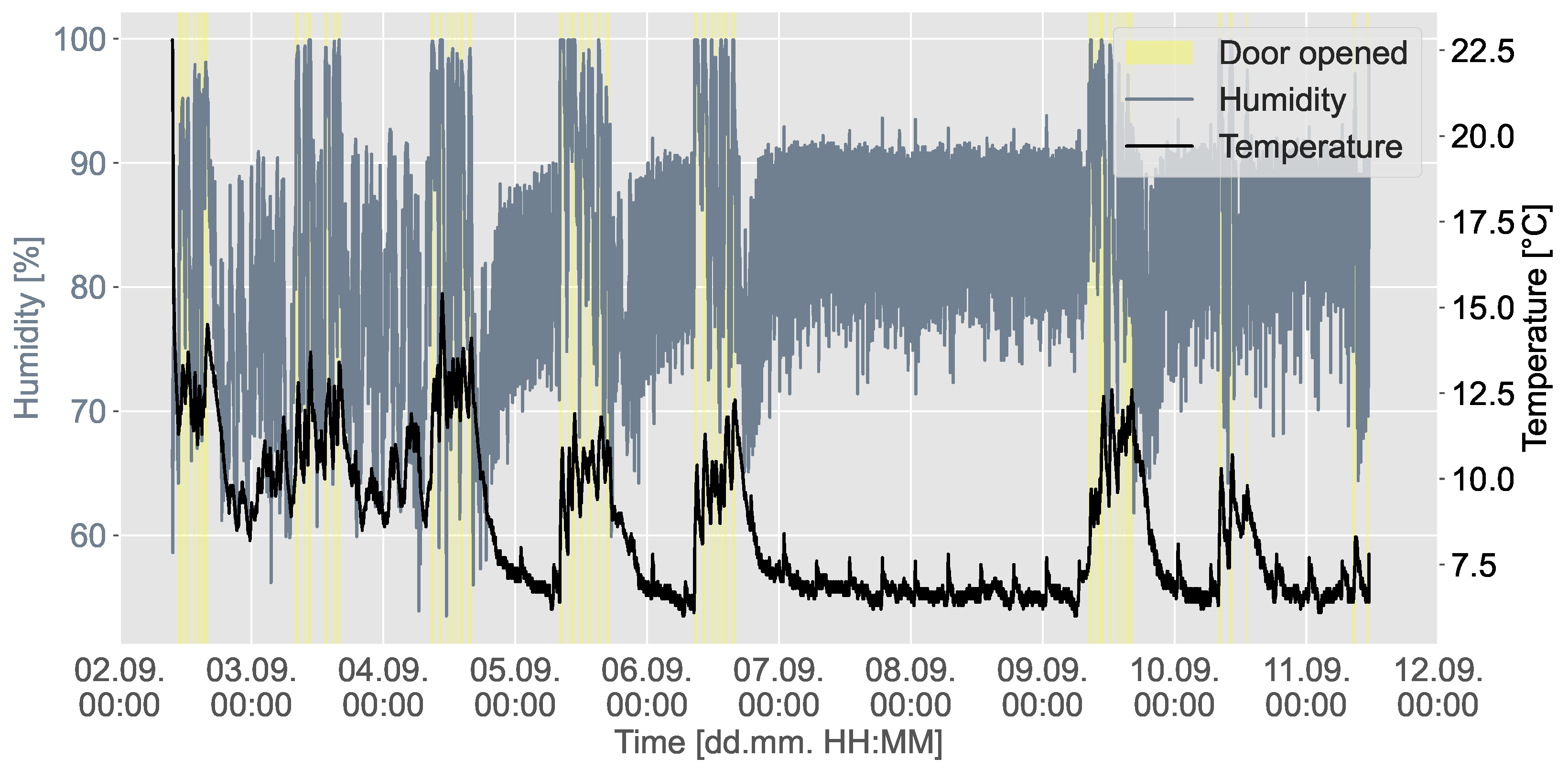
The performance of the approaches for adapting the sensor sampling rate was evaluated using a temperature and humidity time series dataset (https://doi.org/10.5281/zenodo.15130001, accessed on 13 October 2025), gathered and preprocessed as described in [5]. In total, data from nine sensors were used, of which seven sensors were constantly inside the cooling storage, and two sensors were simultaneously brought in and removed from the cooling storage several times to observe the reaction of mobile sensors embedded in water crates to both spatial relocation and ambient changes. Further, the storage room door was occasionally opened to provoke environmental fluctuations to be recorded in the sensor data. Figure 1 shows the sensors’ placement in the cold storage room, and Figure 2 exemplifies the temperature and humidity profiles using non-adaptive data from Sensor 7, which was placed at a lower level in the middle of the cold storage.
Additionally, a brief data analysis of the recorded data was performed in [5] to derive possible parameters for the adaptation logic in the simulations. During data gathering, several sensors had malfunctions, leading to missing data: Sensor 1 exhibited an interruption on 9 September, between 07:04:15 and 08:24:40. Sensor 3 recorded only from 6 September, at 14:08:00, until 11 September, at 11:25:00. Sensor 4 ended recording on 11 September at 03:32:45. Sensor 5 started recording on 9 September, at 16:13:15, and Sensor 9 on 9 September, at 14:00:00. Therefore, Not-a-Number (NaN) values replaced missing values. Table 1 provides an overview of the preprocessed datasets, depicting the non-adaptive data of each sensor.

2.3. Simulations

To evaluate the applicability of adaptive monitoring, sensors that use various approaches to adapt the sensor sampling rate were simulated based on the gathered data. The simulations were executed using Ubuntu 22.04 and Python 3.10.12. Further, the implementations of the approaches used the Python packages pandas (v2.2.3), numpy (v1.26.4), scipy (v1.15.1), scikit-learn (v1.6.1), scikit-fuzzy (v0.5.0), stumpy (v1.13.0), and ruptures (v1.1.9).
The simulated sensors monitored either temperature or humidity. Each approach variant initialized nine individual sensor instances based on the used dataset. The simulation generally followed the steps of initializing the sensor instances, running the simulation, and saving the results afterward. Algorithm 1 depicts the simulation logic in detail. As the simulation works event-based, the next measurement times are stored in a central controller. All sensors scheduled for measuring at the given simulation step perform the simulation actions. First, the sensor outputs the current measurement’s value v and its current sampling rate f. If this is the first measurement, the simulation time t, the measurement value, and the current sampling rate are recorded. Otherwise, the sensor returns the latest reference value r, which is recorded along with the simulation time, the measurement value, and the current sampling rate. Then, the sensor buffer is updated with the current measurement. The sensor sampling rate is set to the highest frequency  f m a x if the current measurement is a NaN value. Otherwise, the approach-specific adaptation logic is called to adapt the sampling rate based on the recent measurements. Finally, the central controller is updated.
Algorithm 1 Simulation logic.
Require: sensor instances, simulation start time t, simulation end time  t e n d
  1:
Initialize controller next_measurement_times for all sensor instances with t 0
  2:
while  t t e n d  do
  3:
    for all sensor instances such that next _ measurement _ time = t  do
  4:
        Retrieve sensor instance and related simulation_data
  5:
         v get _ value ( t ) , f get _ sampling _ rate ( )
  6:
        if simulation_data is empty then
  7:
         Record t, f, and v in simulation_data
  8:
        else
  9:
          r get _ reference _ value ( t )
10:
         Record t, f, v, and r in simulation_data
11:
          buffering ( t , v )
12:
         if  v = NaN  then
13:
              set _ sampling _ rate ( f m a x )
14:
         else
15:
              adapt _ sampling _ rate ( ) {according to specific logic}
16:
         end if
17:
        end if
18:
        Update next_measurement_times
19:
      end for
20:
       t min ( next _ measurement _ times )
21:
end while
22:
return simulation_data
For both the implementation of the simulator and the approaches, the authors used ChatGPT (model GPT-4o) to support the coding process. Furthermore, GenAI provided suggestions for representations of pseudocode and symbolic algorithms in LaTeX, as well as improving runtime efficiency. Due to a lack of available implementations in literature for the implementation of the sensors’ algorithms, the GenAI tool assisted in transferring the algorithms’ descriptions into implementations and code debugging. The authors reviewed and edited all outputs to ensure accuracy and appropriateness. The GenAI tool was not used for data analysis, and the authors made all scientific conclusions.

2.4. Design of Approaches to Adapt the Sensor Sampling Rate

Since the literature investigated several approaches but rarely provided specific implementations, this section describes the implementation of the applied approaches to adapt the sensor sampling rate. Therefore, Section 2.4.1 first explains theoretical foundations for applied techniques. Then, Section 2.4.2 presents the implementation of the approaches to adapt the sensor sampling rate.

2.4.1. Analysis and Optimization Techniques

This work focuses on techniques that analyze data retrospectively and use optimization methods without exhaustive searching to adapt the sensor sampling rate, although they are not limited to retrospective usage. Therefore, this section briefly explains the basics of the analysis and optimization techniques integrated in the approaches and effects of their related parameters. The analysis methods include the exponential weighted moving average, the Bollinger Bands, matrix profiles, change point detection, and Kalman filtering. Considered optimization techniques are the tabu search and the fuzzy logic.
To determine environmental changes, many of the investigated approaches compare the current measurement with past sensor values, computed as the exponential weighted moving average. The exponential weighted moving average reduces the signal noise, whereby the more recent values are also weighted more heavily and thus have a stronger impact [6]. The exponential weighted moving average  v ¯ t  (Equation (1)) weights the current measurement value v stronger, the greater the weighting factor  α is (for 0 < α < 1 ) and reduces the impact of the previous value  v t 1 :
v ¯ t = α · v + ( 1 α ) · v ¯ t 1
In order to consider differences in the sampling time intervals  Δ t , the weighting factor  α is alternatively calculated as follows (Equation (2)):
α t = 1 e α · Δ t
The Bollinger Bands, which originate from the financial sector to analyze stock price trends [18], generate bands around the exponential weighted moving average by  v ¯ t ± σ · s t . The exponential weighted moving standard deviation  s t  (Equation (3)) determines the bandwidth, depending on the sensitivity factor  σ , which controls the weighting of the standard deviation:
s t = α · ( v v ¯ t ) 2 + ( 1 α ) · s t 1 2
Thus, the bandwidth reflects the data’s variance and uncertainty, which becomes greater if the sensor’s signal changes.
The matrix profile of a time series is the z-normalized Euclidean distance between a subsequence of length m and the one closest to it regarding the patterns’ similarity [20]. Thus, matrix profiles provide a representation of the time series’ internal similarity by investigating repetitive and anomalous patterns. Therefore, the subsequences are normalized, and their Euclidean distances are calculated, generating a distance matrix D. Afterward, the lowest distance for each subsequence is determined and stored in a vector, which represents the time series’ matrix profile. Low matrix profile values indicate highly repetitive behavior, while high values highlight unique or anomalous patterns.
Another option to determine changes in the sensor signal is to identify change points in the signal mean using the pruned exact linear time (PELT) algorithm [21]. The PELT algorithm is a search method to determine the optimal segmentation, which approximates the signal piecewise. It is particularly effective when the number of change points is unknown. Therefore, the algorithm minimizes an objective function that balances the goodness-of-fit and model complexity with the set of change points  T , the segmentation  P ( T ) , the penalty factor  ρ , and the cost function  c ( v I )  (Equation (4)):
min T I P ( T ) c ( v I ) + ρ · | T |
The manually set penalty  ρ controls the sensitivity of the detection: lower values lead to the identification of more change points, while higher values result in fewer detected changes by favoring simpler segmentation. Several cost functions for an interval I can be used. This work applies the least squared deviation (L2) between the current measurement value v and the signal mean  v ¯  (Equation (5)):
c ( v I ) = t I | | v v ¯ | | 2 2
A mathematical method for filtering data is the Kalman filter [22]. The Kalman filter is a linear recursive algorithm that smooths data and estimates future values, while also capturing the related estimation errors. The estimate  v ^ is calculated based on the prior estimate  v ^ t 1 and their correction—the Kalman gain  K t —using the latest measurement, weighted by their respective uncertainty, the so-called innovation  ν t  (Equation (6)):
v ^ t = v ^ t 1 + K t ν t
The innovation is the prediction error, quantifying the difference of the current measurement value and the prior estimate weighted with the measurement matrix V, which relates the system state and the measurements (Equation (7)). The Kalman gain determines the correction of the estimate based on the prior error covariance matrix  P t 1 , the measurement noise covariance matrix  R t , the measurement matrix V, and a regularization term to ensure numerical stability using the identity matrix  I n  (Equation (8)). The error covariance matrix is regularly updated following Equation (9).
ν t = v V v ^ t 1
K t = P t 1 V ( V P t 1 V + R t + β I n ) 1 , with β = 10 6
P t = ( I n K t V ) P t 1
The Kalman filter is particularly effective in systems with noisy or incomplete measurements, while keeping the computational effort low due to a reduced number of state variables in the state propagation equation.
In addition to the previously described analysis methods, the tabu search is a meta-heuristic optimization technique for adjusting target parameters [23]. Therefore, the algorithm explores the neighborhood of the current parameter configuration to identify better solutions [24]. A new solution is only selected if its fitness f beats the current (best) parameter fitness  f b e s t . Otherwise, the solution is added to the tabu list of length  n T a b u , which temporarily stores solutions that are ignored in the subsequent searches to prevent cycling and help escape local optima. Thus, the maximum number of iterations  I m a x specifies the maximum number of neighborhood explorations.
Furthermore, fuzzy logic controls system parameters based on heuristic rules [25]. Therefore, fuzzy logic extends classical logic by allowing fuzzy sets in which elements partially belong to a set through a membership function by mapping them to values between 0 and 1 [26]. Building on this concept, fuzzy logic systems apply predefined if–then rules to make decisions in uncertain and ambiguous situations, mimicking human decision-making. A fuzzy logic system consists of a fuzzy rule base, containing the rules to apply, a fuzzification interface that normalizes the input values, a fuzzy inference mechanism, and a defuzzification interface that denormalizes the output values [27]. The inference mechanism maps system inputs to corresponding rules and membership functions, determining the current state and generating the output or adjustment value [28].

2.4.2. Implementation of Approaches

Although this work focuses on adapting the sampling rate, the time interval between two consecutive measurements is actually adapted. The sensor sampling rate is the sampling frequency  f = 1 Δ t , where  Δ t is the time interval. The sampling rate adaptation is initially implemented in a decentralized manner at the sensor level.
In general, there are two basic variants, each defining the adaptation spaces and degrees of freedom in which the adaptations can be conducted. Regarding the adaptation spaces, the first variant, referred to as levels, specifies 12 possible sensor sampling rates (5 s, 10 s, 30 s, 1 min, 2 min, 5 min, 10 min, 15 min, 20 min, 30 min, 60 min, 90 min). The second variant, called bounded, specifies the highest and lowest sensor sampling rates (max. 5 s, min. 90 min), between which the sampling rate can be determined by multiplying or dividing the current sampling rate and rounding to a multiple of 5 s. In both cases, the sampling frequency determined the highest sensor sampling rate during data gathering. The authors of this work determined the lowest sensor sampling rate without in-depth analysis.
Regarding the degrees of freedom, the fixed variant allows for the adaptation of the sensor sampling rate only by moving one step up or down in the predefined list, or by doubling or halving the current sampling rate. In contrast, the variable variant dynamically determines the step width or multiplication factor and divisor depending on the degree of the signal change. However, not all combinations of these variants were applicable across all approaches. Additionally, some studies in the literature propose other, more specific adaptation strategies, which are also considered.
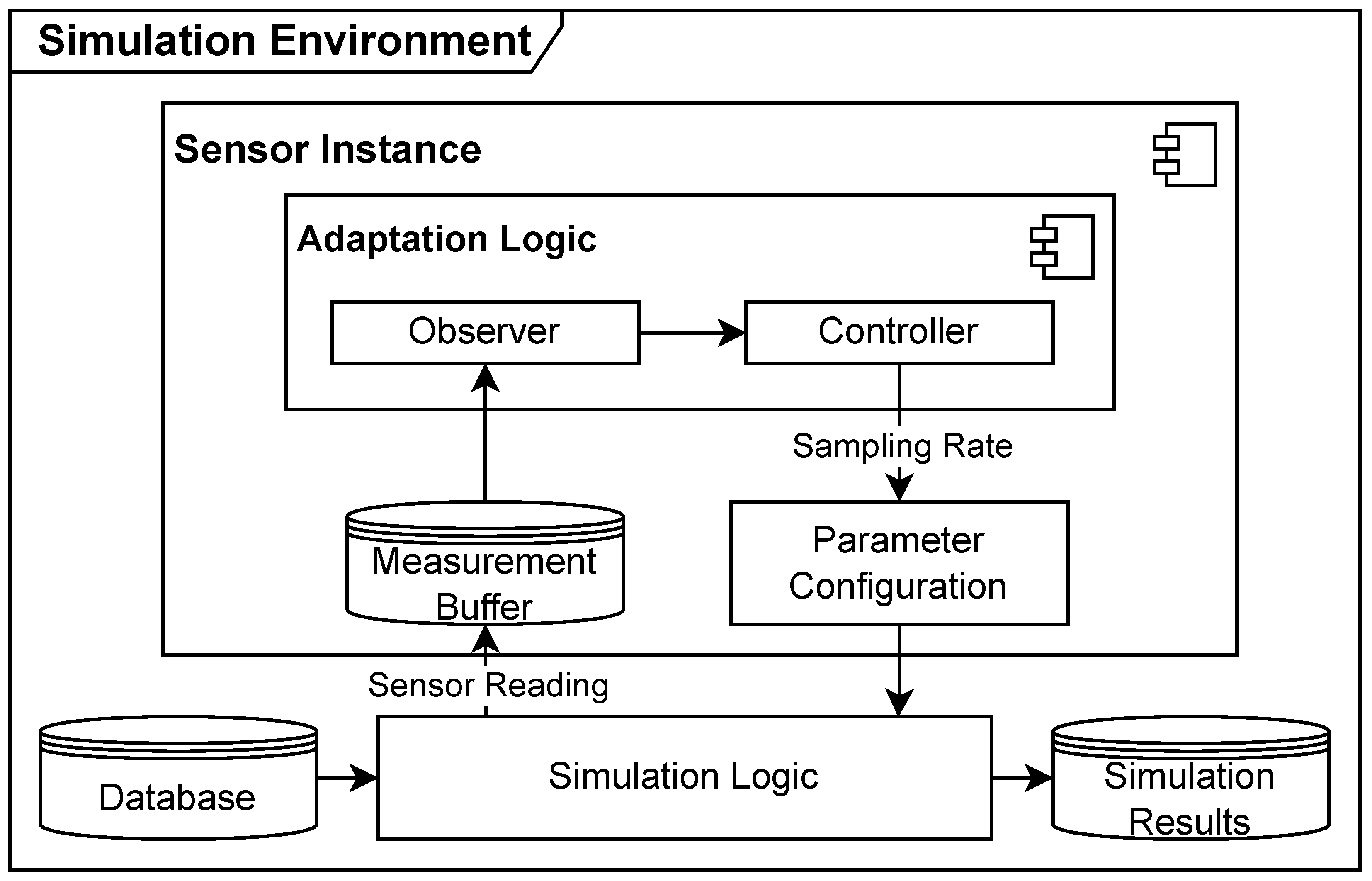
Figure 3 shows the interplay of components in the simulation environment. The simulation logic provides the current sensor measurement to the sensor instance, which stores it in the internal measurement buffer. After storing enough data in the internal sensor buffer, the observer accesses the buffer, calculates a reference value r depending on the applied approach, and determines the degree of signal change  δ s . The controller adapts the sensor sampling rate accordingly to  δ s . Algorithm 2 describes this adaptation logic in more detail. It is worth mentioning that sensors do not communicate with each other or with a central unit. Rather, each sensor instance adapts its sampling rate based on the sensor measurements in a decentralized approach. Moreover, the data transmission rate is the same as the sensor sampling rate to maintain simplicity. Further, the simulation does not consider communication protocols, and the sensors transmit their data on request.
Algorithm 2 General Adaptation Logic.
Require: simulation time t, sensor’s current sampling rate f, sensor value v, buffer
1:
if enough buffer then
2:
     r calculate ( buffer ) {depending on approach, e.g., mean}
3:
     δ s = f ( r , v ) {e.g., deviation}
4:
    if  δ s > allowed _ threshold  then
5:
         set _ sampling _ rate ( f )
6:
    else if  δ s allowed _ threshold  then
7:
         set _ sampling _ rate ( f )
8:
    end if
9:
end if
Generally, two analysis procedures are possible: The retrospective analysis compares the current sensor measurement with past measurements. The resulting degree of signal change determines the adaptation of the sensor sampling rate. The predictive procedures predict the next measurement value and adapt the sensor sampling rate based on the prediction. Although predictive procedure approaches might perform better than retrospective ones as they adapt proactively, their implementation is more challenging in the presence of unknown data. Therefore, this work investigates the applicability of adaptive monitoring approaches using retrospective procedures. Table 2 provides an overview of the approaches and implemented variants as well as the specified parameters.
The simplest approach, called Simple Thresholds, compares consecutive measurements directly. If the measurement remains within a tolerance of the previous one, the sampling rate will be reduced. Conversely, the sampling rate must be increased if the measurement exceeds a threshold. However, the current sampling rate will be kept if the measurement falls within the tolerance and threshold.
A further implemented approach considers an exponential weighted moving average instead of a single measurement to compare the measurements, designated as Mean. Considering different time intervals advances this approach to Mean (Advanced). Similarly, the sampling rate is reduced if the measurements remain in Bollinger Bands and increased if the measurements exceed the Bollinger Bands, following the approach from [18], referred to as Bollinger Bands and Bollinger Bands (Advanced) if considering different time intervals. These approaches also included the specific variants Bounded Band and Bounded Distance, which estimate dynamically the new Δ t using Bollinger Bands and vertical distances between observed and smoothed observed samples, respectively [18]. Additionally, the approach from [29] determines Confidence Intervals using a linear model and adapts the sampling rate if the measurements are in them. Otherwise, the sampling rate is set to the maximum.
Further, an approach determines the Matrix Profiles and increases the sampling rate if the most recent matrix profile value exceeds a threshold. Another approach increases the sampling rate if the analyzing algorithm detects change points using the PELT algorithm. Accordingly, the sampling rate is reduced if the recent matrix profile value is within the threshold or no change points are detected.
Furthermore, an approach determines the most suitable sampling rate using a Tabu Search. The fitness function to calculate the tabu search solution fitness was defined as follows (Equation (10)):
f ( f , v , v t 1 ) = | v v t 1 | · f f m a x , if | v v t 1 |   > 1 | v v t 1 | · f f m a x 1 , if | v v t 1 |   1
To evaluate the fitness value and update the sampling rate accordingly, the asperion criterion A C was determined as follows (Equation (11)), using an aspiration factor ψ :
A C = f b e s t 0.5 · s t , if at least 10 fitness values are available ( 1 ψ ) · f b e s t , otherwise
Additionally, every tabooed candidate f T a b u was excluded from the search for a tabooization time t T a b u (Equation (12)) with scale factor k, in which the candidate was not considered for adaptation:
Δ t T a b u = k · f T a b u
Another approach applied Fuzzy Logic to adapt the sensor sampling rate, following the approach of [25]. Therefore, the current signal change Δ v was determined as the difference between the latest and current measurement values (Equation (13)) and normalized to the range of [ 10 , 10 ] . The normalization interval was chosen to maintain granularity, considering the assumption that large changes in the environmental parameter can occur, e.g., through sudden spatial changes or sensor failures.
Δ v = v t 1 v
The second input parameter was the current sampling rate, which was normalized to the range of [ 1 , 10 ] . The normalization interval was chosen to avoid zero and provide a large enough mapping space. Depending on the predefined fuzzy rules, the output f o u t is determined and added to the current sampling rate to adjust it, before the new sampling rate is denormalized again and applied for the next measurement (Equation (14)):
f ˜ n e w = f ˜ + f o u t
Additionally, one approach applied a Kalman Filter, following the work of [22]. The authors of [22] calculated the estimation error δ t i (Equation (15)) and subsequently the total error Δ i (Equation (16)), which is then used to determine the adjustment of the sampling rate as follows (Equation (17)):
δ t i = trace ν t i · ( v i ) 1 2
Δ i = j = 0 T 1 δ j i w j j = 0 T 1 w j
f n e w = f + ϕ · ( 1 e Δ i λ λ )
The total error Δ i is calculated using weights w j = 1 j + 1 with j = 0 for the most recent error to increase the effect of the most recent error. The exponent Δ i λ λ , limited to [ 10 , 7 ] to avoid exceeding the sampling rate limits, determines the new sampling rate with the parameter λ = 0.75 and the scaling factor ϕ = 2 .
As this work focuses on evaluating the general behavior and potential of these approaches, rather than proposing novel methods or achieving performance-optimized implementations, the parameters were initially set as follows, based on empirical evaluations: The sensor’s internal buffer length was n b u f = 60 , which equals 5 min if the maximum sampling rate is set. The absolute thresholds θ were 0.3 °C for temperature and 5% the humidity, as the median peak heights were between 0.9 °C and 14.1 °C, and 25.7% and 32.9%, respectively. The tolerance τ was set to 0.1 °C for temperature and 2% for humidity, as τ needs to be smaller than θ . The thresholds for matrix profiles θ M P were 1 for the temperature matrix profiles and 0.3 for the humidity matrix profiles, as the median matrix profile values were between 1.6 and 3.2 and 0.3 and 0.5, respectively. The smoothing factor for exponentially weighted calculations was set to α = 0.75 to give more weight to the latest values. The sensitivity factor was set to σ = 2 to meet the confidence level γ = 0.95 . The penalty for PELT’s prediction was ρ = 1000 , as a higher value reduced the number of detected change points but also resulted in longer runtime, and values ρ > 1000 showed no further improvement in empirical trials. The tabu search ran for a maximum of 10 iterations ( I m a x ) with a tabu list length of n T a b u = 3 , an aspiration factor of ψ = 0.1 , and a scaling factor of k = 1.5 to control the duration of the sampling rate tabulation.

3. Results

To assess the general applicability, this section presents the simulation results, examining the performance of the investigated approaches (RQ2). Since the performance is hard to determine using a single metric, the reduction of the gathered data (Section 3.1), the observation accuracy of critical events (Section 3.2), the responsiveness as the number of adaptations (Section 3.3), and adaptation metrics (Section 3.4), determining the approach’s efficiency, are considered.

3.1. Reduction of Gathered Data (RQ2.1)

The reduction of gathered data C is the normalized difference between the non-adaptive data length at maximum sampling rate n t o t a l , without considering NaN values, and the data length of the adaptive approach n (Equation (18)), similar to [6,19]:
C = n t o t a l n a d a p t n t o t a l
Consequently, C = 0 means that the approach did not reduce the data, while C = 1 indicates a full reduction (i.e., no data were gathered at all).
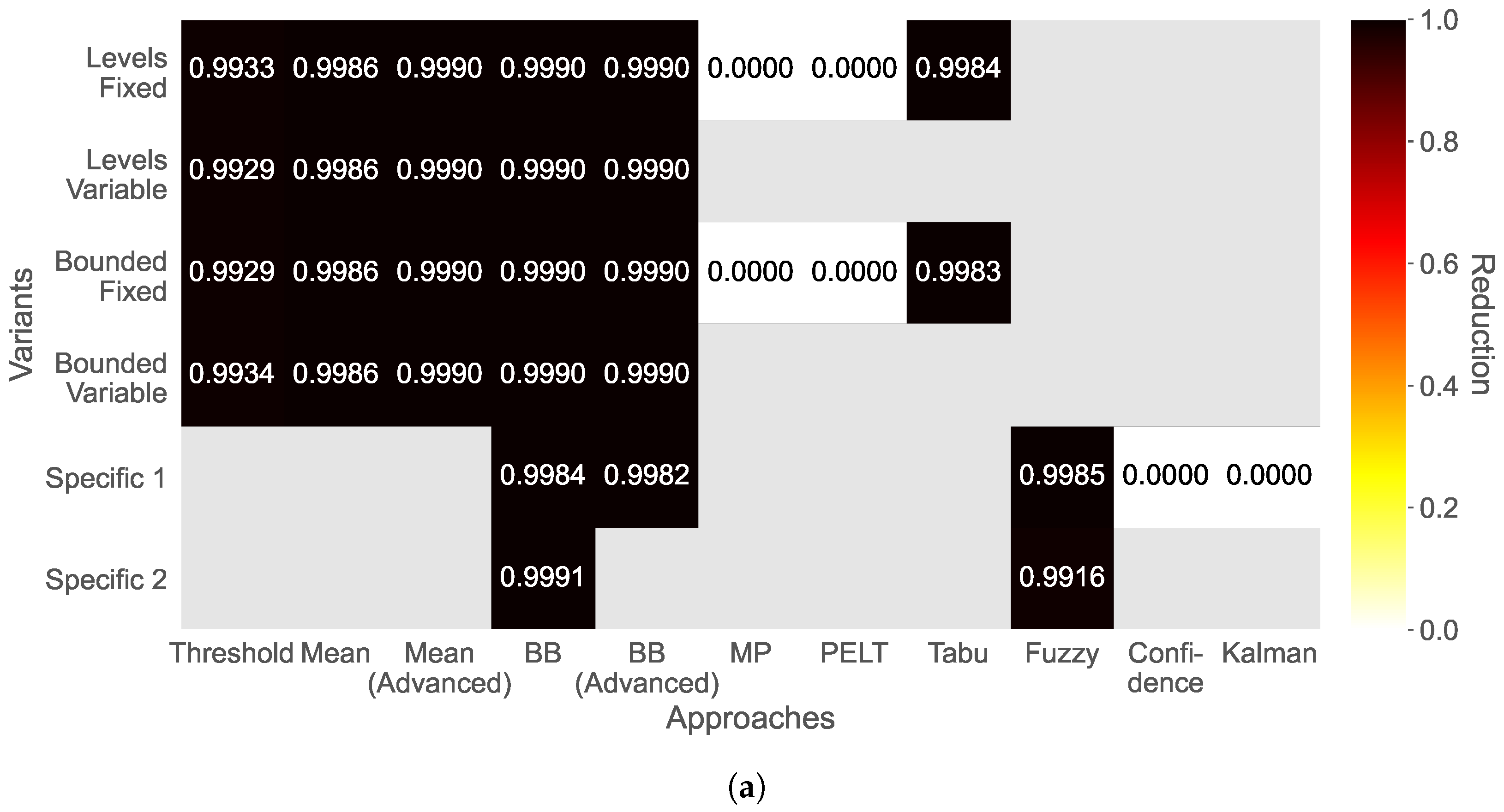
Figure 4 shows the reduction of gathered data C of the different approaches. Although the study aims to investigate the general applicability of adaptive monitoring for food monitoring rather than determining the best-performing approach, displaying the median of all sensors per variant allows for comparison of the approaches to derive their strengths and weaknesses. Moreover, the reduction indicates the general functionality of the approaches, revealing that the approaches Matrix Profiles (MP), PELT, Confidence Intervals, and the Kalman Filter failed for both parameters, temperature and humidity (no reduction at all). This does not necessarily mean that these approaches are not applicable, but may also be reasoned by an inadequate selection of the configured parameters. However, further brief attempts with other configurations were also unsuccessful. Therefore, a deeper analysis might be part of future work due to the large variety of approaches that have been investigated, but these approaches will not be considered further.
Concerning the temperature (Figure 4a), the other approaches and variants strongly reduce the gathered data compared to the non-adaptive data, all close to a reduction of C = 1 . The Fuzzy Logic’s bounded variant reduced the data the least (0.9916), and the Bollinger Bands’ (BB) specific Bounded Distance variant reduced the data the most (0.9991). Regarding the humidity (Figure 4b), the approaches and variants show similar results in terms of reduction potential. The Bollinger Bands’ specific variant Bounded Distance reduced the data again the most (0.9991). However, the least-reducing approach was the Tabu Search, with a reduction of 0.8427 for the levels fixed variant and 0.8596 for the bounded fixed variant.

3.2. Observation Accuracy (RQ2.2)

While reducing the amount of data gathered improves data analysis efficiency and reduces the sensor’s energy consumption, the data must be gathered sufficiently to monitor the environment, particularly critical events. Therefore, the second qualitative metric focused on the timestamps of local extremes in the time series, which were logged manually during the experiments and further determined using the find_peaks() function from the Python module scipy.signal, as described in [5]. These timestamps were merged with timestamps of actions performed during data gathering, building dynamic change intervals ( D C I ) in which critical events happen (cf. yellow time windows in Figure 2). The observation accuracy ( O A ) is the quotient of the observed D C I and the D C I in the non-adaptive sensor data (Equation (19)), corresponding to the recall metric in machine learning settings, whereas recall is usually determined in binary form:
O A = D C I a d a p t D C I t o t a l
Hence, an O A = 0 means that the approach did not monitor any crucial event, while an O A = 1 indicates monitoring all critical events.
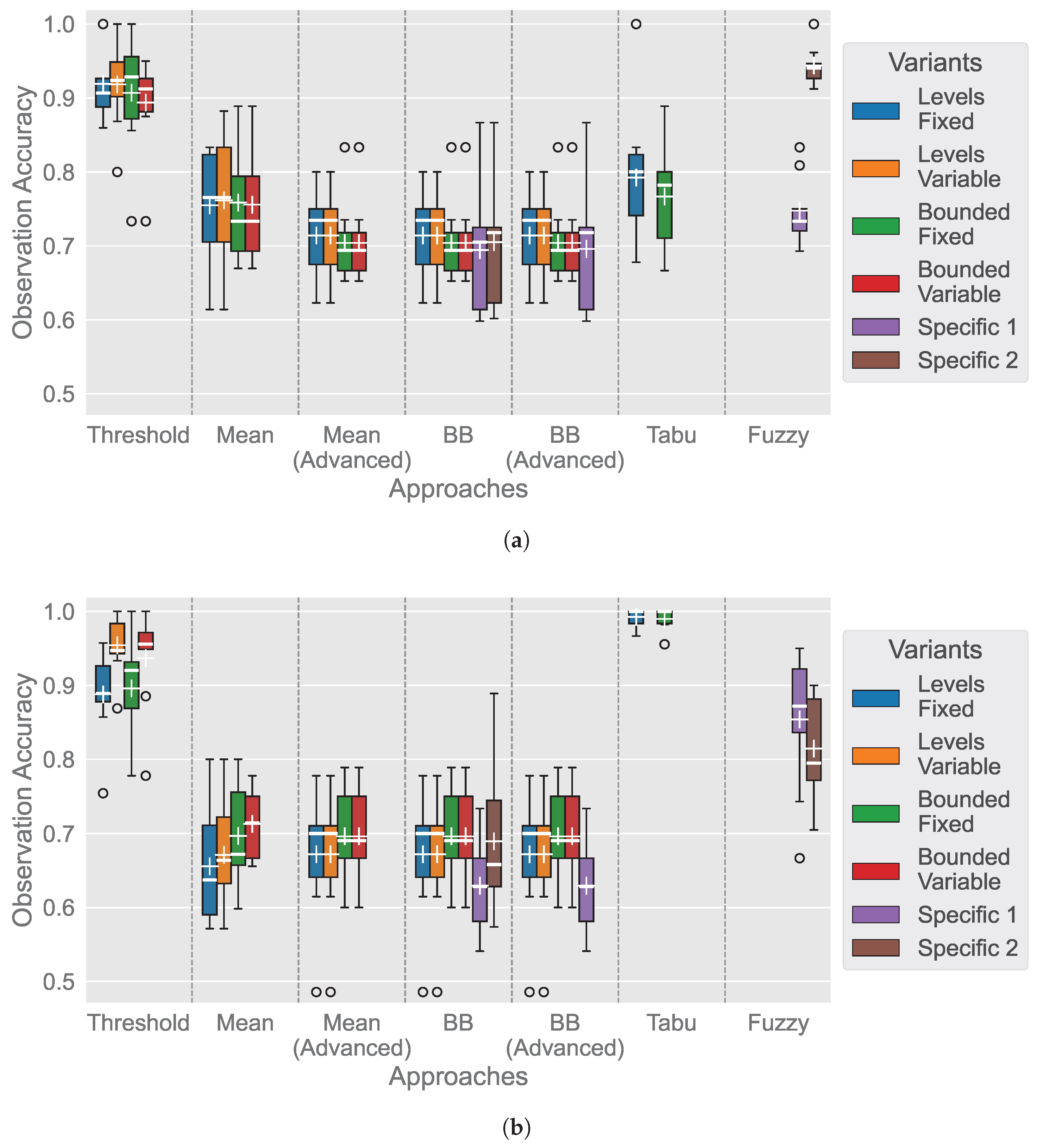
Figure 5 shows the observation accuracy of gathered data from the different approaches. As the figure shows different box sizes, revealing differences in the observation accuracy depending on the sensor’s non-adaptive data, the observation accuracy is compared using the median values in the following.
Concerning the temperature (Figure 5a), the Fuzzy Logic’s bounded variant has the highest observation accuracy (0.9407). Further, the Simple Threshold approach has a high observation accuracy, especially the bounded fixed and levels variable variants (0.9286 and 0.9237, respectively). The other approaches’ observation accuracy is between 0.6939 (bounded variants of the approaches Mean, Bollinger Bands, and Bollinger Bands (Advanced)) and 0.8000 (levels fixed variant of the Tabu Search approach). Worth mentioning is that some variants of the approaches Simple Thresholds, Tabu Search, and Fuzzy Logic achieved an observation accuracy of 1.0000 for a few sensors, meaning all critical events could be detected. However, the observation accuracy for some sensors of the specific variant Bounded Band of the Bollinger Bands and Bollinger Bands (Advanced) approaches was only 0.5982.
Regarding the humidity data (Figure 5b), both Tabu Search variants achieved the highest observation accuracy (1.0000). Additionally, the Simple Threshold approach has a high observation accuracy, particularly for the variable variants (bounded variable 0.9558 and levels variable 0.9474). The fixed variants of the Simple Threshold approach performed slightly worse, still achieving observation accuracies of 0.9204 for the bounded fixed variant and 0.8889 for the levels fixed variant. The Fuzzy Logic’s levels variant has a higher observation accuracy than the bounded variant (0.8718 and 0.7949, respectively). The approaches Mean, Mean (Advanced), Bollinger Bands, and Bollinger Bands (Advanced) have observation accuracies between 0.6286 (Bounded Band variant of the Bollinger Bands and Bollinger Bands (Advanced) approaches) and 0.7143 (for the bounded variable variant of the Mean approach). Similar to the temperature data, some variants of the Simple Thresholds approach also achieved an observation accuracy of 1.0000 for a few datasets. However, they also contained outliers with an observation accuracy below 0.5 for the levels variants of the approaches Mean (Advanced), Bollinger Bands, and Bollinger Bands (Advanced), meaning that less than half of the critical events were detected.

3.3. Number of Adaptations (RQ2.3)

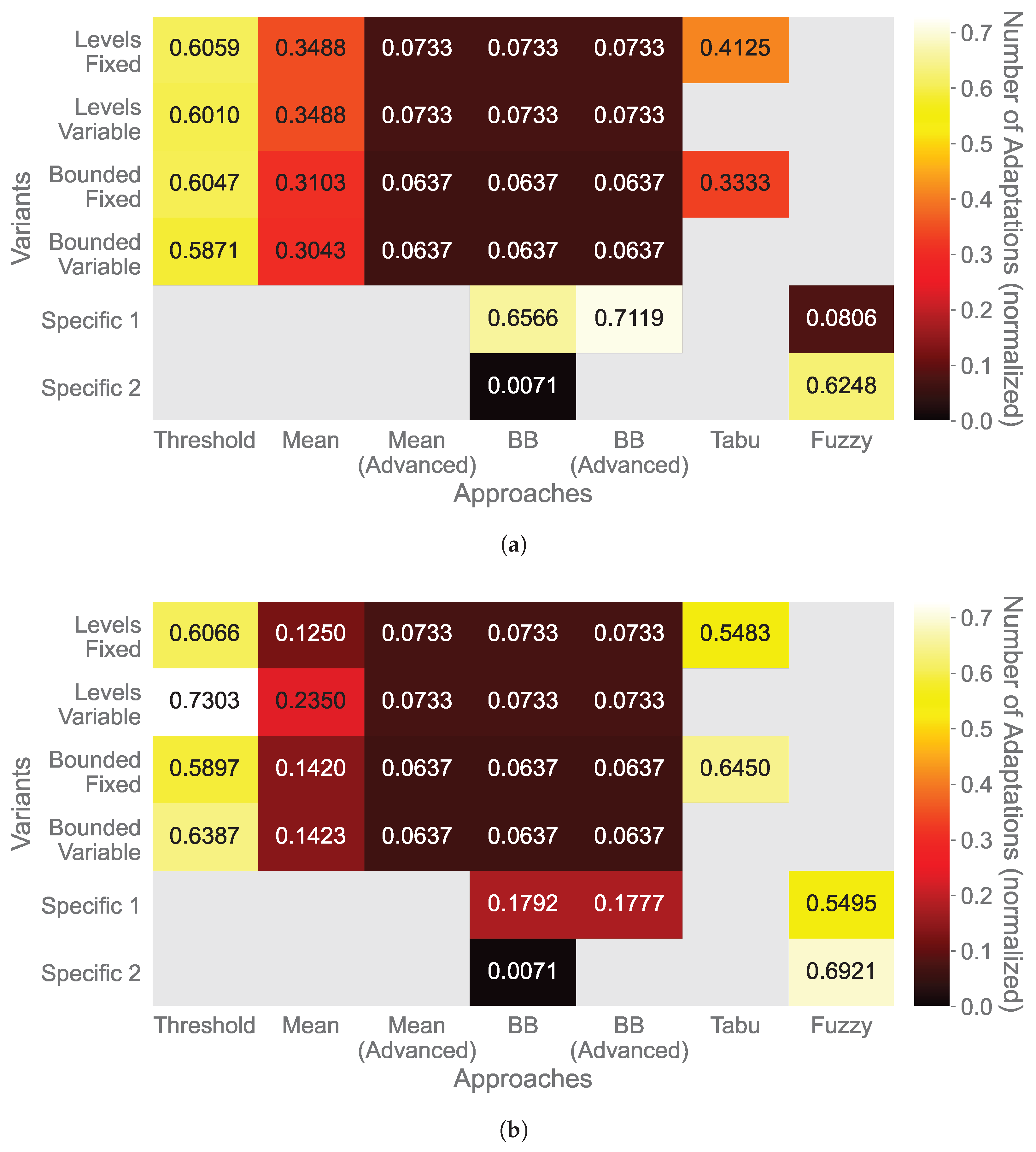
The approaches’ responsiveness to environmental changes is derived from the number of adaptations they exhibit. A high responsiveness (a high adaptation number) indicates that an approach adapts fast to changes in the data, i.e., it adapts closely after a signal changes significantly. Figure 6 shows the medians of the number of adaptations, normalized by the length of the adaptive dataset.
For the temperature signals (Figure 6a), the Bollinger Bands (Advanced) Bounded Band variant adapted the most (0.7719), followed by the Bollinger Bands Bounded Band and the Fuzzy Logic’s bounded variants (0.6566 and 0.6248, respectively). Furthermore, the Simple Thresholds approach adapted rather often with numbers between 0.5871 (bounded variable variant) and 0.6059 (levels fixed variant). The Mean and Tabu Search approaches had medium-low adaptations (between 0.3043 for the Mean bounded variable variant and 0.4125 for the Tabu Search levels fixed variant). The approaches Mean (Advanced), Bollinger Bands, Bollinger Bands (Advanced), and the Fuzzy Logic’s levels variant adapted much less with numbers of adaptations below 0.1.
Regarding the humidity data (Figure 6b), the Mean (Advanced), Bollinger Bands, and Bollinger Bands (Advanced) approaches exhibit the same number of adaptations as for the temperature, except Bounded Band variants, which had much lower numbers (0.1792 for the Bollinger Bands approach and 0.1777 for the Bollinger Bands (Advanced) approach). Additionally, the Mean approach adapted less (between 0.1250 for levels fixed and 0.1423 for bounded variable), although the levels variable variant (0.2350) was more active than the other variants. The Simple Thresholds approach yielded similar results to the temperature (between 0.5897 for bounded fixed and 0.6387 for bounded variable), but the levels variable variant also showed a higher level of adaptation (0.7303). Moreover, the Tabu Search approach (0.5483 for levels fixed and 0.6450 for bounded fixed) and the Fuzzy Logic’s levels variant (0.5495) have higher adaptation numbers compared to the temperature.

3.4. Adaptation Efficiency (RQ2.4)

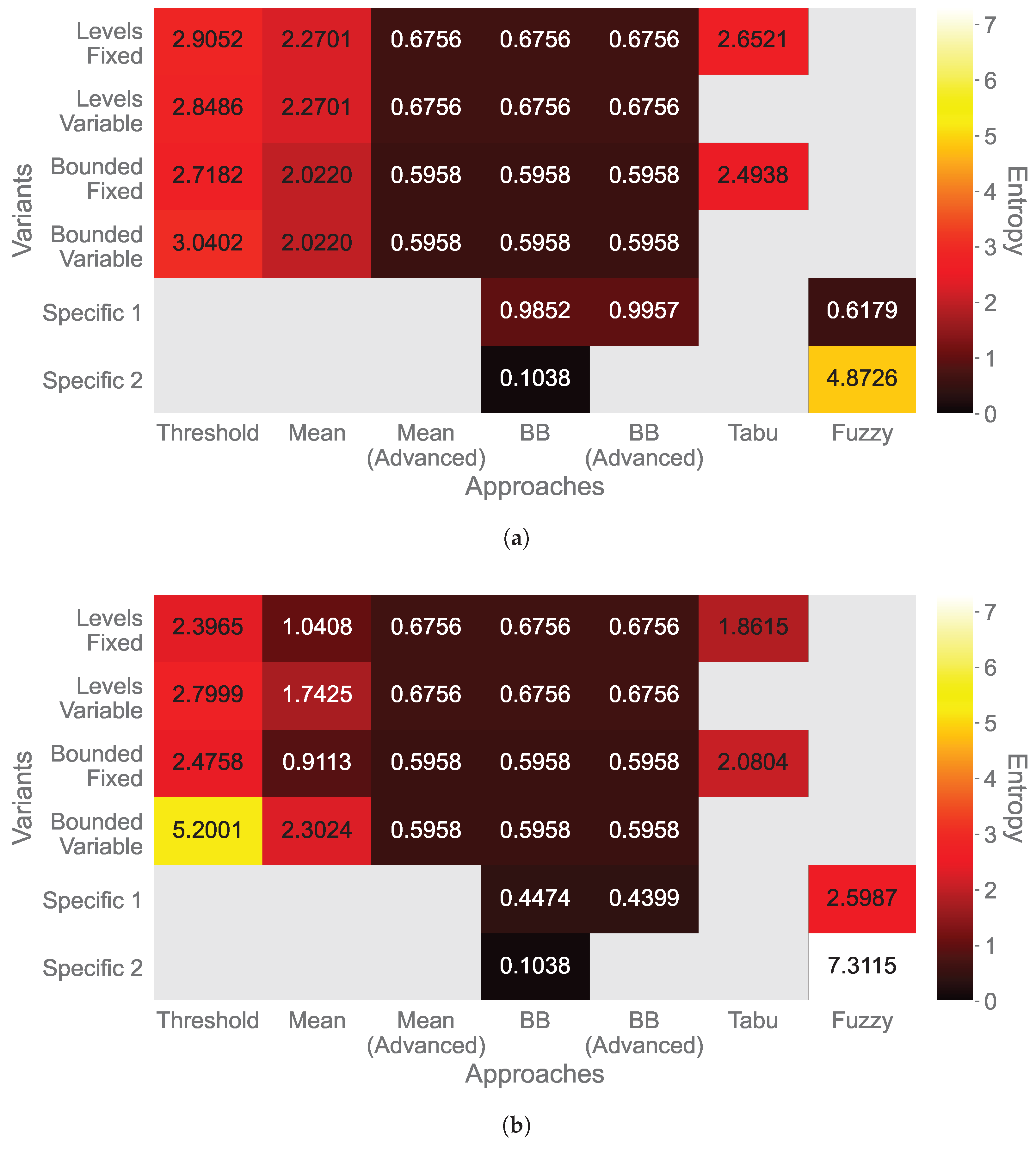
Shannon’s Entropy H ( X ) and the number of oscillation phases N O evaluate the adaptation efficiency by indicating the configuration certainty and stability [30]. Figure 7 shows the medians of Shannon’s Entropy, which is calculated using the sampling rates as system states X. A low entropy signifies a high certainty regarding the probability of specific system states to occur, meaning that only a few dominant states are likely to occur due to overly relaxed parameter configurations. In contrast, a high entropy denotes a low predictability of system states, implying that the system frequently explores a wide range of sampling rates due to too tightly constrained parameters. Hence, neither a low nor a high, but a medium-low entropy is preferable.
The maximum entropy is determined by H m a x = log 2 ( n ) , where n is the number of unique sampling rates. Thus, the maximum entropy of the levels fixed variants is H m a x ( 12 ) = 3.5850 , and for the bounded fixed variants, H m a x ( 11 ) = 3.4594 . The maximum entropy is less consistent for the variable variants since the number of unique sampling rates varies due to the more flexible calculation of new sampling rates, resulting in higher possible maximum entropy values. However, this example intends only to facilitate the comparative assessment of the entropy and promote its comprehensibility.
Regarding the temperature (Figure 7a), the Fuzzy Logic’s bounded variant has the highest entropy (4.8726), while the Bollinger BandsBounded Distance variant has the lowest (0.1038). The Tabu Search approach has a medium-high entropy (2.6521 for the levels and 2.4938 for the bounded variant). Further, the entropy of the Mean approach is slightly lower (2.2701 for both levels and 2.0220 for both bounded variants), and the entropy for the Simple Thresholds approach is slightly higher (between 2.7182 for the bounded fixed and 3.0402 for the bounded variable variant).
Concerning the humidity (Figure 7b), the entropy of the Fuzzy Logic’s bounded variant is also the highest (7.3115), even higher than for the temperature data. The Bollinger BandsBounded Distance variant also has the lowest entropy (0.1038). Compared to the entropy for the temperature data, the Tabu Search approach is lower (1.8615 for the levels and 2.0804 for the bounded variant) but achieves much higher observation accuracies. The entropy of the Fuzzy Logic’s levels variant is also higher (2.5987), as is the observation accuracy for the humidity. Moreover, the entropy of the Simple Thresholds approach is lower for the humidity than for the temperature, except for the bounded variable variant, which is comparably high (5.2001).
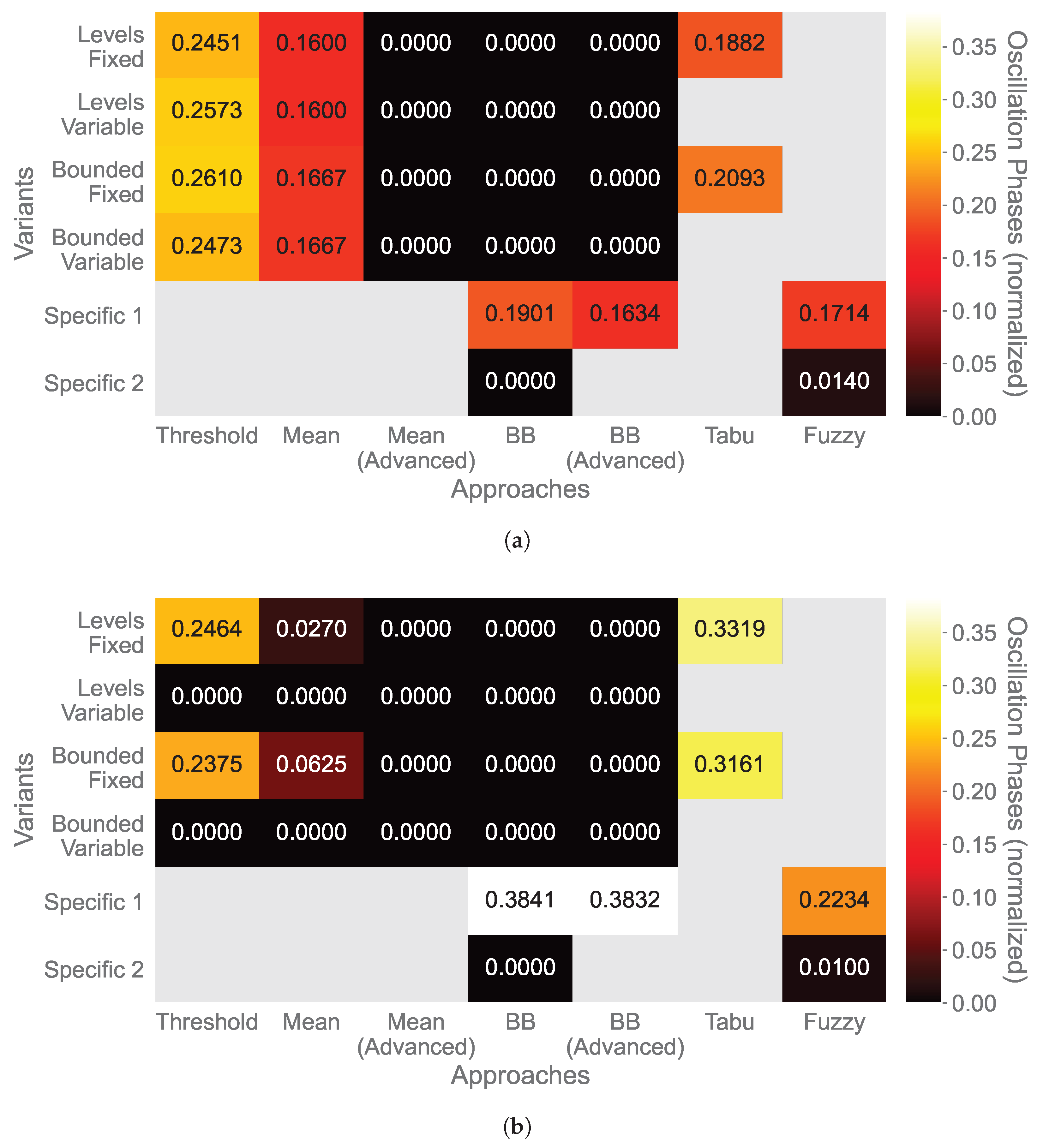
Figure 8 shows the number of oscillation phases. An oscillation phase occurs if the sampling rates change from one to another and back to the previous sampling rate in successive measurement cycles of a sensor. If the sampling rate consecutively returns to the second rate, this is still counted as one oscillation phase. The number of oscillations is normalized by the number of adaptations. A low number of oscillations indicates a stable system. In contrast, many oscillations refer to an unstable system that tends to over-correct its adaptations. As for the entropy, neither a low nor a high, but a medium number of oscillations is preferable.
Regarding the temperature (Figure 8a), the Simple Thresholds approach exhibits a distinctly higher number of oscillations than the other approaches, being between 0.2473 for the bounded variable and 0.2610 for the bounded fixed variants. Further notable oscillations occur for the approaches Tabu Search (0.1882 for the levels fixed and 0.2093 for the bounded fixed variant), Mean (0.1600 for both levels and 0.1667 for both bounded variants), and the Fuzzy Logic’s bounded variant (0.0140). No or one oscillation phase was determined for the other approaches. Although the entropy is medium for the Simple Thresholds approach, it tends to oscillate, but it also achieves a high observation accuracy while massively reducing the data. In contrast, the Fuzzy Logic’s bounded variant has a similar observation accuracy and data reduction, but the number of oscillations is much lower. However, the entropy is the highest for this approach.
Concerning the humidity (Figure 8b), the Tabu Search approach has the highest number of oscillations, which is even higher compared to the highest number for the temperature data (0.3161 for the bounded fixed and 0.3319 for the levels fixed variant), but also reaches the highest observation accuracy while having a medium entropy. For the Simple Thresholds approach, the number of oscillations is higher for the fixed variants (0.2464 for the levels and 0.2375 for the bounded variant) and 0.0000 for the variable variants. Considering the observation accuracy, the variants with fewer oscillations are preferable. However, the bounded variable variant has a much higher entropy than the levels variable variant. For the Fuzzy Logic approach, the number of oscillations of the levels variant is higher than for the bounded variant (0.2234 and 0.0100, respectively). However, the bounded variant also has the highest entropy over all. Thus, determining the best-performing approach is not possible, and one must consider some trade-offs.

4. Discussion

In the following, Section 4.1 briefly discusses the approach implementation. Afterward, Section 4.2 analyzes the performance of different approaches to assess the general applicability of adaptive monitoring in the context of food storage. Subsequently, Section 4.3 discusses options to improve the adaptation approaches. Finally, Section 4.4 closes the discussion by exploring threats to validity.

4.1. Architecture of Adaptation Approaches

In general, the monitoring activity must be adapted or intensified when environmental conditions change, such as temperature or humidity fluctuations, e.g., due to a failure of the cooling system or the movement of products from storage to distribution. However, if the environmental conditions are stable, the sensor sampling rate can be decreased to reduce the energy demand. Further, adapting the sensor sampling rate is unnecessary if the current sampling rate allows sufficient monitoring of the environment. As literature reveals, several approaches are possible to adapt the sensor sampling rate, but vary in their scope and implementation level. Therefore, this section answers the following research question:
  • RQ1: How can adaptive monitoring be applied to adapt the sensor sampling rate?
Possible adaptation approaches include adaptation logics that are implemented into the sensor nodes [12,18,19,31] as well as centralized analyzing mechanisms [10,14,15,16,32]. Additionally, there are hybrid approaches that centrally perform a prior analysis of the current state and determination of boundary conditions [13], as well as the validation of the applied adaptation and feedback provision [17], while the sampling rate is adapted locally at the sensor node. While a central approach represents a potential single point of failure that could disrupt the entire system [12], a decentralized, local approach might lack comprehensive situation-awareness and lead to incorrect adjustments.
However, as this work aims to investigate the general applicability of approaches to adapt the sensor sampling rate, the approaches investigated in this work were implemented at the sensor level. Moreover, this work represents an initial evaluation of different approaches regarding the potential and challenges in food monitoring. The dynamic and complex character of food supply chains requires an independent and decentralized adaptation logic, as sensor nodes operate in changing environments with limited or intermittent connectivity to a central controller. Additionally, integrating communication and centralized coordination demands a system-of-systems integration [5] and, therefore, increases the system complexity. Hence, this is outside of this work’s scope, but will be considered for future work.

4.2. Performance Analysis

To investigate the general applicability of adaptive monitoring to adapt the sensor sampling rate, the performance of the chosen approaches is analyzed, answering RQ2:
  • RQ2: What is the performance of the investigated approaches?
Therefore, analyzing data reduction (RQ2.1), observation accuracy (RQ2.2), responsiveness (RQ2.3), and adaptation efficiency (RQ2.4) provides a comprehensive view to assess the performance.
In general, no approach or specific variant outperformed the others, except for those that did not reduce the gathered data at all. Comparing the observed parameters or underlying data, the reduction for the Simple Thresholds approach and the Fuzzy Logic’s bounded variant was smaller for the humidity than for the temperature. In contrast, the reduction for the approach Mean (except the bounded variable variant) and the variants Bounded Distance of the Bollinger Bands and Bollinger Bands (Advanced) approaches, as well as the Fuzzy Logic’s bounded variant, were greater for the humidity compared to the temperature. The reduction of the other approaches was the same for both monitored parameters.
Thus, the approaches reduced the data for both parameters and show potential for reducing different data types. Still, the results reveal dependencies on the data characteristics, e.g., data noise, regarding the reduction potential. Nevertheless, the reduction potential is more substantial than other approaches described in the literature, which were between 0.70 and 0.75 [6,19]. However, this comparison should be treated with caution, as the reference sampling rate is significantly lower (2.5 min) [19] or not specified [6]. Furthermore, the high reduction potential suggests that a sampling rate of 5 s is not necessary permanently and can therefore be decreased, therby reducing the data and further emphasizing the useful application of adaptive monitoring.
However, balancing the data reduction and the monitoring of critical events is crucial since an overly large reduction could result in missing crucial events. In fact, the approaches reduce the data volume greatly, but at the same time, the reduction raises concerns regarding the accuracy in detecting critical events. A too-reduced sampling rate could miss changes in the sensor’s signal and not adapt fast enough.
Thus, the observation accuracy reveals big differences in the performance of some approaches. Particularly, the Tabu Search approach observes more critical events on the noisier humidity data, as the data is less reduced. In contrast, the Fuzzy Logic’s bounded variant performs better when the data has less noise, although the data reduction is similar (0.9916 for the temperature data and 0.9963 for the noisier humidity data).
However, while the observation accuracy indicates whether measurements were taken during a critical event, it does not provide any information about the extent of data gathering during these events and the quality, i.e., whether the local maximum was recorded directly or an outer value of the D C I . Therefore, future work should revise the calculation of the observation accuracy, including changes in the sensor sampling rate. In addition, the observation accuracy of some approaches might be improved by optimizing the parameter configuration for each approach and monitored parameter, enabling a fairer comparison of the approaches.
Analyzing the number of adaptations demonstrates the effectiveness of the approaches depending on the underlying data. Furthermore, the adaptation numbers indicate the responsiveness to signal changes and also relate to the observation accuracy, as a higher adaptation number also results in a higher observation accuracy. However, the number of adaptations itself does not reveal anything about the adaptation efficiency, as it could also be excessively responsive and overreacting. Therefore, Shannon’s Entropy and the number of oscillation phases provide better insights into the efficiency, as analyzed in the following.
Regarding adaptation efficiency, the approaches Mean (Advanced), Bollinger Bands, and Bollinger Bands (Advanced) have low entropy values, indicating that the parameter configurations are probably too relaxed. In contrast, the parameter configuration for the Fuzzy Logic’s bounded and the Simple Thresholds bounded variable variants are too strict, as their entropy values are high. Furthermore, the parameter configuration for the remaining approaches is also not optimal, although it is reasonably efficient. Moreover, the analysis of oscillations reveals that the Bollinger Bands’ and Bollinger Bands (Advanced) levels variants have high oscillation numbers, but only one oscillation phase in absolute terms. Further, the approaches Simple Thresholds and Tabu Search tend to oscillate for the temperature and humidity signals, respectively. Thus, these approaches switch often between two sampling rates in consecutive steps, indicating a suboptimal parameter configuration or a challenging detection and subsequent adaptation in borderline cases. Since oscillations imply continuous adaptation and, consequently, prior analysis of the system state, this also increases the computational effort and subsequently reduces efficiency. Hence, future work might not only include the optimization of the parameter configuration, but also its adaptation during the monitoring process.
In summary, Table 3 provides an overview of the strengths and weaknesses of the successfully implemented approaches. The table highlights the trade-offs that must be considered when selecting the approaches. High observation accuracy comes with low stability, and vice versa. Additionally, a high reduction and high adaptation efficiency yield low observation accuracy. For instance, the approaches Simple Thresholds and Fuzzy Logic offer a good balance between data reduction and observation accuracy for the temperature data. The Tabu Search approach is excellent for accuracy on noisy data, such as the humidity signal, but achieves a low level of data reduction. Further, the statistic-based approaches Mean, Mean (Advanced), Bollinger Bands, and Bollinger Bands (Advanced) strongly reduce the data, but react slowly, resulting in low observation accuracies.
Additionally, the approaches’ performances could be further improved by optimizing the parameter configurations. Therefore, future work includes fine-tuning the initially initiated configurations. Moreover, the configurations could be adapted during runtime depending on the given scenario. For instance, if the monitoring system detects that the products are moving and leaving the stationary storage environment, a parameter configuration can be selected that reacts more quickly to changes in the environment and monitors them appropriately. Thus, the performance of the monitoring system could be further enhanced, ensuring strong data reduction while maintaining high observation accuracy and high adaptation efficiency. Therefore, demonstrating the functionality of these approaches is a first step toward implementing this complex food monitoring system.

4.3. Applicability Discussion

After analyzing the approaches’ performance, the general applicability of adaptive monitoring approaches in the context of food monitoring will be discussed, addressing the following research question:
  • RQ3: Is adaptive monitoring applicable in dynamic and unpredictable environments?
First of all, while a lower static sampling rate would also reduce the volume of data collected, it cannot respond to dynamic environmental changes. As a result, critical events or environmental changes may remain undetected or insufficiently monitored, limiting the accurate prediction of the remaining food shelf life. Hence, adaptive monitoring approaches, adapting the sensor sampling rate in response to environmental changes, enable not only the identification of when deviations occurred during food storage, but also the assessment of their extent. Information about the values and duration of exposure is necessary for accurate and reliable shelf life predictions. Thus, adaptive monitoring facilitates efficient data collection for assessment. Using this high-quality database and integrating it into spoilage models or (machine learning based) analyzing algorithms can result in an improved quality prediction. Especially when considering energy-constrained machine learning for analyzing food storage conditions [33], e.g., during transportation, the fact of data reduction is even more important as it can also reduce analysis time and effort, resulting in reduced computational power required for machine learning.
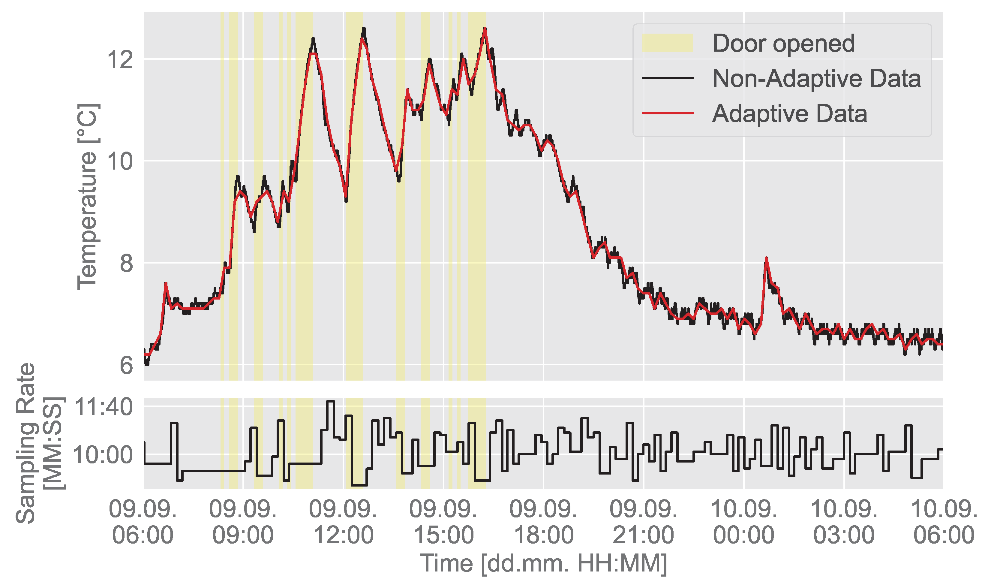
The approaches Simple Thresholds, Mean, Mean (Advanced), Bollinger Bands, Bollinger Bands (Advanced), Tabu Search, and Fuzzy Logic were successfully implemented. Notably, Simple Thresholds, Tabu Search, and Fuzzy Logic achieved a more substantial data reduction compared to methods discussed in the previous literature, but they have a lower reference sampling rate [6,19], while achieving a higher observation accuracy [6]. Figure 9 illustrates an example of the data collected using Fuzzy Logic’s bounded variant for Sensor 7.
However, the performance and adaptability of these approaches are highly dependent on the characteristics of the monitored data. The Fuzzy Logic’s bounded variant achieves the highest observation accuracy for the temperature data, but far lower for the humidity data. Regarding the humidity data, the Tabu Search approach achieves the highest observation accuracy but also the lowest reduction. Thus, no single approach is suitable for all scenarios, corresponding to the No-Free-Lunch-Theorem [34]. Accordingly, the approach should be selected depending on the given scenario, e.g., another approach might be preferable for transportation than for stationary storage. Therefore, the system can analyze its current performance, determine the best-fitting approach at a higher level, and then initiate adaptation if appropriate [4,5].
Further, analyses of Shannon’s entropy and the number of oscillations indicate the configuration certainty and stability. For instance, the approaches Simple Thresholds for temperature and Tabu Search for humidity exhibit relatively high oscillation rates with medium entropy values, while also achieving high observation accuracies. Therefore, selecting the approach involves trade-offs between data reduction and adaptation efficiency, as the accuracy of observations is crucial for monitoring critical events.
Moreover, static parameter configurations limit responsiveness. For instance, the statistic-based approaches Mean, Mean (Advanced), Bollinger Bands, and Bollinger Bands (Advanced) also yielded substantial data reduction but achieved lower observation accuracies than the other approaches. Considering the adaptation efficiency, these approaches show low entropy and a low number of oscillations. Thus, sudden changes remain undetected, and the approaches react too slowly to monitor critical events because the buffer is too large. To overcome this, dynamically adapting the buffer length with the current sampling rate is beneficial. Moreover, the extent of the environmental changes varies, requiring situation-aware adaptations to adequately react to those changes and ensure the monitoring of critical events. Therefore, a learning component could be integrated to provide globally optimized strategies [35].
However, the adaptation approach should be further selected depending on the available resources. In addition to the monitoring activity itself, the adaptation algorithms also require energy, differing depending on their complexity. For instance, while the Simple Threshold approach compares two values, the statistic-based approaches Mean, Mean (Advanced), Bollinger Bands, and Bollinger Bands (Advanced) further calculate the moving averages, which need buffer storage and computational resources. Furthermore, an optimization-based approach, such as Tabu Search, demands higher computational resources and thus consumes more energy due to its iterative search. Thus, the parameter configuration, such as the maximum number of iterations, could be used to control their demands and adjust them to the available resources.
Finally, this work focused on reactive, retrospective adaptation approaches. Future work considers the investigation of predictive methods such as AdaM [6], FAST [36], ARIMA [37], Fisher Information and Gaussian Process Regression [38], and learning-based approaches like artificial neural networks [19], aiming to enable proactive adaptation. Nevertheless, adaptive monitoring is generally applicable for adapting the sensor sampling rate in dynamic and unstable environments, such as food storage.

4.4. Threats to Validity

This work followed a structured approach to investigate the general applicability of adaptive monitoring in the context of food monitoring, comparing different approaches to adapt the sensor sampling rate. Therefore, various approaches were implemented, and their performance was compared. However, some threats to validity remain.
First, the initial parameter configuration for the different approaches was chosen empirically. Therefore, optimizing the parameter configuration prior to sensor instantiation could improve the results. Moreover, optimizing the adaptation planning could identify new parameters during runtime [23].
Further, the data sampling was synchronized to facilitate the implementation of the different adaptive monitoring approaches. Thus, the results only represent a simplified implementation. Additionally, this work did not consider requirements or challenges for communication and the localization of sensors in the storage room. Decentralized information exchange and situational awareness could further improve performance in such environments.
Although the data were gathered using DHT22 sensors measuring temperature and humidity simultaneously, this work evaluated adaptive monitoring approaches for both parameters separately. Adapting the sensor sampling rate based on fused sensor data might further increase the approaches’ accuracy.
Additionally, energy consumption was not monitored and evaluated. This work used data reduction as a surrogate for the energy savings, but communication and adaptations also demand energy, which is currently not considered. Thus, computational and communication overhead should be evaluated in future work to assess the performance of adaptation approaches. Furthermore, monitoring the energy level of the sensors would also contribute to the performance of the approaches.
Finally, this work defined the observation accuracy as the quotient of observed and given dynamic change intervals. However, the observation accuracy only states if measurements were taken in the dynamic change intervals, but it does not indicate how well the critical events were monitored. Thus, some measurements could be executed randomly in the dynamic change intervals without adapting to the environmental change, leading to a higher observation accuracy. Nevertheless, we could show that the approaches adapted differently; hence, the current observation accuracy is adequate to indicate differences in the performance at the current stage.

5. Conclusions

This work investigated the general applicability of adaptive monitoring approaches to adapt the sensor sampling rate in a dynamic and unpredictable environment. The approaches were evaluated based on temperature and humidity data in a food storage room. Therefore, it is crucial to monitor critical events while reducing the amount of data gathered to improve the data analysis efficiency and reduce the sensor’s energy demand in mobile applications. The approaches performed differently depending on the underlying data, but achieved high observation accuracies and substantial data reduction. However, adaptation metrics revealed further optimization potential. Additionally, further approaches that proactively adapt the sensor sampling rate will be investigated in future work. Further, investigating the adaptive monitoring approaches for other application scenarios, such as process monitoring, is considered [39].
Moreover, in addition to environmental changes, the physical location of food products changes throughout the different stages of the food supply chain, resulting in various combinations of food products and packaging. Thus, adapting the structure of the monitoring system should be investigated in addition to adapting the sensor sampling rate [4]. Therefore, the sensor’s activity must be adjusted to provide complete information on the product’s environment. Considering these aspects, an adaptive monitoring system for food monitoring is built.

Author Contributions

Conceptualization, E.H. and C.K.; methodology, E.H. and C.K.; software, E.H.; validation, E.H., D.J., P.S. and C.K.; formal analysis, E.H.; investigation, E.H.; resources, C.K.; data curation, E.H.; writing—original draft preparation, E.H.; writing—review and editing, E.H., D.J., P.S. and C.K.; visualization, E.H.; supervision, C.K.; project administration, C.K.; funding acquisition, C.K. All authors have read and agreed to the published version of the manuscript.

Funding

This research is funded by the Deutsche Forschungsgemeinschaft (DFG, German Research Foundation) grant number 516601628.

Institutional Review Board Statement

Not applicable.

Informed Consent Statement

Not applicable.

Data Availability Statement

The original data presented in the study are openly available in Zenodo at https://doi.org/10.5281/zenodo.15130001 (accessed on 13 October 2025). The software used for the simulations and to create the results is openly available on Gitlab at https://gitlab.foodinformatics.uni-hohenheim.de/zomer71/adaptive-monitoring-simulator-sampling-rate (accessed on 13 October 2025).

Acknowledgments

We thank Florian Stoll for his help during data gathering and Mario Jekle and his team from the Department of Plant-Based Foods, University of Hohenheim, particularly Robert Fribus, for their support during data gathering and for providing the cooling storage room. During the preparation of this manuscript/study, the author(s) used Grammarly for the purposes of checking spelling and grammar and ChatGPT (model GPT-4o) for generating and improving the source code of the simulation. The authors have reviewed and edited the output and take full responsibility for the content of this publication.

Conflicts of Interest

The authors declare no conflicts of interest.

Abbreviations

The following abbreviations are used in this manuscript:
IoTInternet of Things
MLOCMulti-Level Observer/Controller architecture
NaNNot-a-Number value
OCOrganic Computing
RQresearch question
WSNWireless Sensor Network
δ s degree of signal change
rreference value
fsensor sampling rate
f m a x maximal sensor sampling rate
tsimulation time
vsensor measurement value
The following simulation parameters are used in this manuscript:
α smoothing factor
δ s degree of signal change
γ confidence level
I m a x maximum iterations for tabu search
kscale factor
n b u f sensor’s internal buffer length
n T a b u    tabu list length
ψ aspiration factor
ρ penalty for PELT prediction
σ deviation factor
θ absolute threshold
θ M P threshold for matrix profiles
τ tolerance
The following formula signs are used in this manuscript:
A C aspiration criterion
Creduction of gathered data
c ( v I ) cost function
D C I dynamic change intervals
H ( X ) Shannon’s Entropy
K t Kalman gain
Iinterval
I n identity matrix
ndata length of adaptive approach
n t o t a l     non-adaptive data length
N O number of oscillation phases
P ( T ) segmentation
P t error covariance matrix
O A observation accuracy
R t measurement noise covariance matrix
T set of change points
Xsystem states
Vmeasurement matrix
ν t Kalman innovation

References

  1. United Nations Environment Programme. Food Waste Index Report 2024. Think Eat Save: Tracking Progress to Halve Global Food Waste. 2024. Available online: https://wedocs.unep.org/20.500.11822/45230 (accessed on 25 April 2025).
  2. Herzberg, R.; Schmidt, T.G.; Schneider, F. Characteristics and Determinants of Domestic Food Waste: A Representative Diary Study across Germany. Sustainability 2020, 12, 4702. [Google Scholar] [CrossRef]
  3. Müller, P.; Schmid, M. Intelligent Packaging in the Food Sector: A Brief Overview. Foods 2019, 8, 16. [Google Scholar] [CrossRef] [PubMed]
  4. Henrichs, E.; Krupitzer, C. Towards a Self-Adaptive, Real-Time Monitoring System for Food Quality Assessment. In Proceedings of the 2024 IEEE International Conference on Autonomic Computing and Self-Organizing Systems Companion (ACSOS-C), Aarhus, Denmark, 16–20 September 2024; pp. 178–179. [Google Scholar] [CrossRef]
  5. Henrichs, E.; Stoll, F.; Krupitzer, C. Towards Self-Adaptive Monitoring of Storage Environments with Distributed Sensor Systems. In Proceedings of the 2025 IEEE International Conference on Autonomic Computing and Self-Organizing Systems Companion (ACSOS-C), Tokyo, Japan, 29 September–3 October 2025; pp. 85–90. [Google Scholar]
  6. Trihinas, D.; Pallis, G.; Dikaiakos, M.D. AdaM: An adaptive monitoring framework for sampling and filtering on IoT devices. In Proceedings of the 2015 IEEE International Conference on Big Data (Big Data), Tokyo, Japan, 29 October–1 November 2015; pp. 717–726. [Google Scholar] [CrossRef]
  7. Albrecht, A.; Ibald, R.; Raab, V.; Reichstein, W.; Haarer, D.; Kreyenschmidt, J. Implementation of Time Temperature Indicators to Improve Temperature Monitoring and Support Dynamic Shelf Life in Meat Supply Chains. J. Packag. Technol. Res. 2020, 4, 23–32. [Google Scholar] [CrossRef] [PubMed]
  8. Zavala, E.; Franch, X.; Marco, J. Adaptive monitoring: A systematic mapping. Inf. Softw. Technol. 2019, 105, 161–189. [Google Scholar] [CrossRef]
  9. Moui, A.; Desprats, T.; Lavinal, E.; Sibilla, M. Information Models for Managing Monitoring Adaptation Enforcement. In Proceedings of the ADAPTIVE 2012: The Fourth International Conference on Adaptive and Self-Adaptive Systems and Applications, Nice, France, 22–27 July 2012; pp. 44–50. [Google Scholar]
  10. Alippi, C.; Anastasi, G.; Di Francesco, M.; Roveri, M. An Adaptive Sampling Algorithm for Effective Energy Management in Wireless Sensor Networks with Energy-Hungry Sensors. IEEE Trans. Instrum. Meas. 2010, 59, 335–344. [Google Scholar] [CrossRef]
  11. Bhuiyan, M.Z.A.; Wu, J.; Wang, G.; Wang, T.; Hassan, M.M. E-Sampling: Event-Sensitive Autonomous Adaptive Sensing and Low-Cost Monitoring in Networked Sensing Systems. ACM Trans. Auton. Adapt. Syst. 2017, 12, 1–29. [Google Scholar] [CrossRef]
  12. Pal, A.; Kant, K. On the Feasibility of Distributed Sampling Rate Adaptation in Heterogeneous and Collaborative Wireless Sensor Networks. In Proceedings of the 2016 25th International Conference on Computer Communication and Networks (ICCCN), Waikoloa, HI, USA, 1–4 August 2016; pp. 1–9. [Google Scholar] [CrossRef]
  13. Habib, C.; Makhoul, A.; Darazi, R.; Couturier, R. Real-time Sampling Rate Adaptation based on Continuous Risk Level Evaluation in Wireless Body Sensor Networks. In Proceedings of the 2017 IEEE 13th International Conference on Wireless and Mobile Computing, Networking and Communications (WiMob), Rome, Italy, 9–11 October 2017; pp. 1–8. [Google Scholar] [CrossRef]
  14. Qi, X.; Keally, M.; Zhou, G.; Li, Y.; Ren, Z. AdaSense: Adapting sampling rates for activity recognition in Body Sensor Networks. In Proceedings of the 2013 IEEE 19th Real-Time and Embedded Technology and Applications Symposium (RTAS), Philadelphia, PA, USA, 9–11 April 2013; pp. 163–172. [Google Scholar] [CrossRef]
  15. Islam, M.N.A.; Cleland-Huang, J.; Vierhauser, M. ADAM: Adaptive Monitoring of Runtime Anomalies in Small Uncrewed Aerial Systems. In Proceedings of the 19th International Symposium on Software Engineering for Adaptive and Self-Managing Systems (SEAMS), Lisbon, Portugal, 15–16 April 2024; pp. 44–55. [Google Scholar] [CrossRef]
  16. Stadler, M.; Vierhauser, M.; Cleland-Huang, J. Towards flexible runtime monitoring support for ROS-based applications. In Proceedings of the 4th International Workshop on Robotics Software Engineering (RoSE), Pittsburgh, PA, USA, 9 May 2022; pp. 43–46. [Google Scholar] [CrossRef]
  17. Vierhauser, M.; Wohlrab, R.; Stadler, M.; Cleland-Huang, J. AMon: A domain-specific language and framework for adaptive monitoring of Cyber—Physical Systems. J. Syst. Softw. 2023, 195, 111507. [Google Scholar] [CrossRef]
  18. Kulau, U.; van Balen, J.; Schildt, S.; Büsching, F.; Wolf, L. Dynamic sample rate adaptation for long-term IoT sensing applications. In Proceedings of the 2016 IEEE 3rd World Forum on Internet of Things (WF-IoT), Reston, VA, USA, 12–14 December 2016; pp. 271–276. [Google Scholar] [CrossRef]
  19. Wang, X.; Jabbari, A.; Jedermann, R.; Laur, R.; Lang, W. Adaptive Data Sensing Rate in Ad-hoc Sensor Networks for Autonomous Transport Application. In Proceedings of the 2010 13th International Conference on Information Fusion, Edinburgh, UK, 26–29 July 2010; pp. 1–8. [Google Scholar] [CrossRef]
  20. Law, S.M. STUMPY: A Powerful and Scalable Python Library for Time Series Data Mining. J. Open Source Softw. 2019, 4, 1504. [Google Scholar] [CrossRef]
  21. Truong, C.; Oudre, L.; Vayatis, N. Selective review of offline change point detection methods. Signal Process. 2020, 167, 107299. [Google Scholar] [CrossRef]
  22. Jain, A.; Chang, E.Y. Adaptive Sampling for Sensor Networks. In Proceedings of the 1st International Workshop on Data Management for Sensor Networks: In Conjunction with VLDB 2004, Toronto, ON, Canada, 30 August 2004; pp. 10–16. [Google Scholar] [CrossRef]
  23. Henrichs, E.; Lesch, V.; Straesser, M.; Kounev, S.; Krupitzer, C. A literature review on optimization techniques for adaptation planning in adaptive systems: State of the art and research directions. Inf. Softw. Technol. 2022, 149, 106940. [Google Scholar] [CrossRef]
  24. Ennigrou, M.; Ghédira, K. New local diversification techniques for flexible job shop scheduling problem with a multi-agent approach. Auton. Agents Multi-Agent Syst. 2008, 17, 270–287. [Google Scholar] [CrossRef]
  25. Hernandez, E.A.; Chidester, M.C.; George, A.D. Adaptive Sampling for Network Management. J. Netw. Syst. Manag. 2001, 9, 409–434. [Google Scholar] [CrossRef]
  26. Angarita-Zapata, J.S.; Alonso-Vicario, A.; Masegosa, A.D.; Legarda, J. A Taxonomy of Food Supply Chain Problems from a Computational Intelligence Perspective. Sensors 2021, 21, 6910. [Google Scholar] [CrossRef]
  27. Lee, G.J.; Fortes, J.A.B. Improving Data-Analytics Performance via Autonomic Control of Concurrency and Resource Units. ACM Trans. Auton. Adapt. Syst. 2019, 13, 1–25. [Google Scholar] [CrossRef]
  28. Chuang, S.N.; Chan, A.T. Dynamic QoS Adaptation for Mobile Middleware. IEEE Trans. Softw. Eng. 2008, 34, 738–752. [Google Scholar] [CrossRef]
  29. Padhy, P.; Dash, R.K.; Martinez, K.; Jennings, N.R. A utility-based sensing and communication model for a glacial sensor network. In Proceedings of the Fifth International Joint Conference on Autonomous Agents and Multiagent Systems, Hakodate, Japan, 8–12 May 2006; pp. 1353–1360. [Google Scholar] [CrossRef]
  30. Lange, J.; Schweizer, P.; Henrichs, E.; Kaendler, L.; Tomforde, S.; Krupitzer, C. A Measurement Framework at Global and Local Levels for Hybrid Organic Computing Systems. In Proceedings of the Architecture of Computing Systems, Kiel, Germany, 22–24 April 2025; Tomforde, S., Krupitzer, C., Vialle, S., Suarez, E., Pionteck, T., Eds.; Springer: Cham, Switzerland, 2025; pp. 283–297. [Google Scholar]
  31. Zhang, Y.; He, S.; Chen, J.; Sun, Y.; Shen, X.S. Distributed Sampling Rate Control for Rechargeable Sensor Nodes with Limited Battery Capacity. IEEE Trans. Wirel. Commun. 2013, 12, 3096–3106. [Google Scholar] [CrossRef]
  32. Bandyopadhyay, S.; Tian, Q.; Coyle, E. Spatio-temporal sampling rates and energy efficiency in wireless sensor networks. IEEE/ACM Trans. Netw. 2005, 13, 1339–1352. [Google Scholar] [CrossRef]
  33. Krupitzer, C.; Stein, A. Unleashing the Potential of Digitalization in the Agri-Food Chain for Integrated Food Systems. Annu. Rev. Food Sci. Technol. 2024, 15, 307–328. [Google Scholar] [CrossRef]
  34. Wolpert, D.; Macready, W. No free lunch theorems for optimization. IEEE Trans. Evol. Comput. 1997, 1, 67–82. [Google Scholar] [CrossRef]
  35. Schweizer, P. A System Model for Flexible Multi-Objective Adaptation Planning in Hybrid Self-Adaptive and Self-Organizing Systems. In Proceedings of the Architecture of Computing Systems, Kiel, Germany, 22–24 April 2025; Tomforde, S., Krupitzer, C., Vialle, S., Suarez, E., Pionteck, T., Eds.; Springer: Cham, Switzerland, 2025; pp. 357–366. [Google Scholar]
  36. Fan, L.; Xiong, L. Real-Time Aggregate Monitoring with Differential Privacy. In Proceedings of the 21st ACM International Conference on Information and Knowledge Management, Maui, HI, USA, 29 October–2 November 2012; pp. 2169–2173. [Google Scholar] [CrossRef]
  37. Ezeora, O.S.; Heckenbergerova, J.; Musilek, P. A new adaptive sampling method for energy-efficient measurement of environmental parameters. In Proceedings of the 2016 IEEE 16th International Conference on Environment and Electrical Engineering (EEEIC), Florence, Italy, 7–10 June 2016; pp. 1–6. [Google Scholar] [CrossRef]
  38. Kho, J.; Rogers, A.; Jennings, N.R. Decentralized Control of Adaptive Sampling in Wireless Sensor Networks. ACM Trans. Sens. Netw. 2009, 5, 1–35. [Google Scholar] [CrossRef]
  39. Jox, D.; Borsum, C.; Hummel, D.; Hinrichs, J.; Krupitzer, C. Enhancing dairy processing with machine learning and domain knowledge: A combined analysis of offline and time series data. J. Food Eng. 2025, 391, 112423. [Google Scholar] [CrossRef]
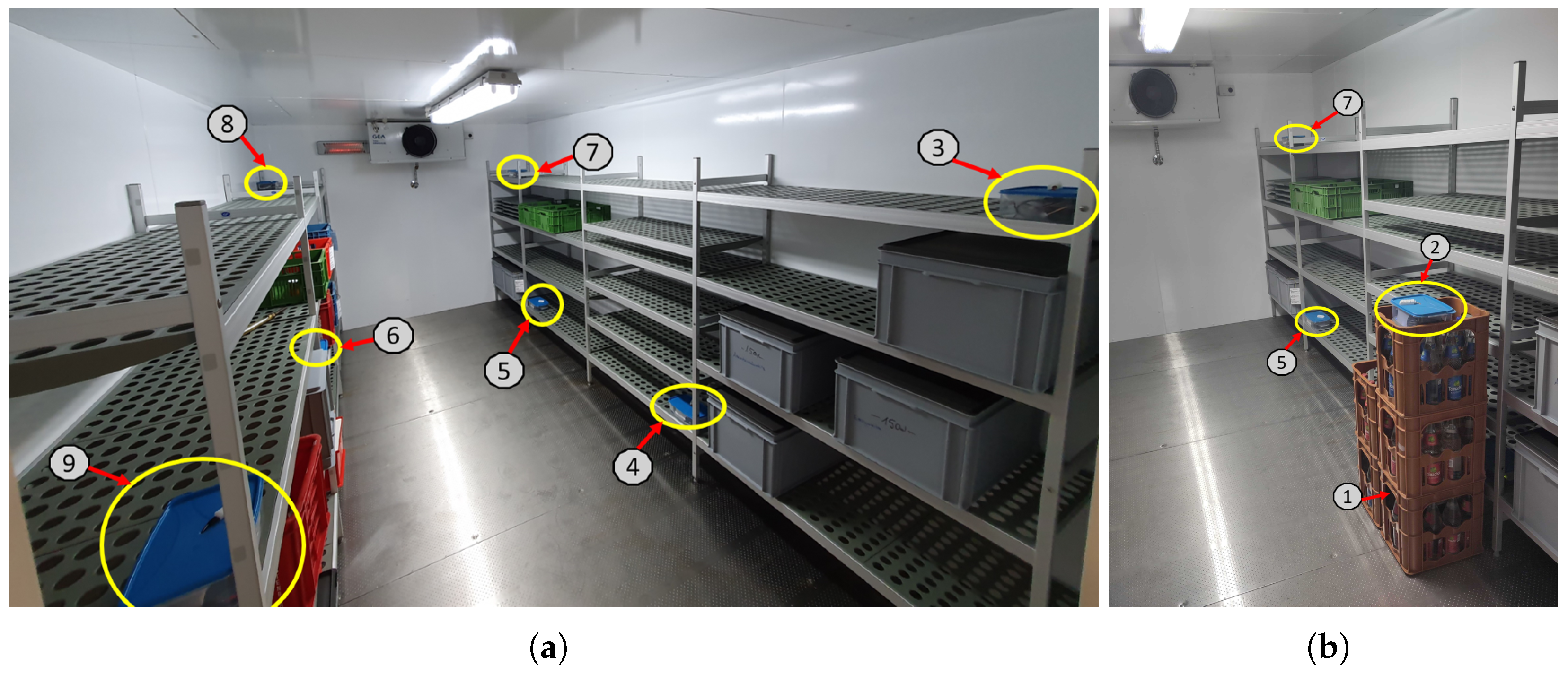
Figure 1. Placement of data loggers in the cold storage room—(a) Permanently installed (Sensors 3 to 9) and (b) temporarily removed (movable) sensors (Sensors 1 and 2) that were placed in crates, simulating food packages.
Jsan 14 00102 g001
Figure 2. Temperature and humidity profiles exemplified by the data from Sensor 7. Periods are highlighted in which actions were performed during data collection to create critical events.
Jsan 14 00102 g002
Figure 3. System architecture of the simulation, focusing on the sensor instances and adaptation logic.
Jsan 14 00102 g003
Figure 4. Median of the gathered data reduction C for all sensors for monitoring (a) temperature and (b) humidity. The variants Specific 1 and Specific 2 refer to specific variants according to the order in Table 2, e.g., Bounded Band and Bounded Distance of the Bollinger Bands approach.
Jsan 14 00102 g004aJsan 14 00102 g004b
Figure 5. Observation accuracy O A with median (−) and mean (+) values of approaches for monitoring (a) temperature and (b) humidity.
Jsan 14 00102 g005
Figure 6. Number of adaptations of approaches for monitoring (a) temperature and (b) humidity.
Jsan 14 00102 g006
Figure 7. Shannon’s entropy H ( X ) of approaches for monitoring (a) temperature and (b) humidity.
Jsan 14 00102 g007
Figure 8. Number of oscillations of approaches for monitoring (a) temperature and (b) humidity.
Jsan 14 00102 g008
Figure 9. Exemplary comparison of the non-adaptive and adaptive data and presentation of the respective sensor sampling rate using the Fuzzy Logic bounded variant for Sensor 7.
Jsan 14 00102 g009
Table 1. Overview of the dataset and key statistics for each sensor, including raw data time coverage, number of valid readings after preprocessing (excluding NaN), missing data intervals due to sensor malfunctions (NaN Start and End, if occurred), and characteristics of temperature and humidity signals, such as overall values, signal peaks, and matrix profiles.
Sensors123456789
Metadata Length
w/o NaN
155,869156,83584,444151,16831,101156,835156,835156,83532,700
NaN Start09.09.24
07:04:15
02.09.24
09:35:25
11.09.24
03:32:45
02.09.24
09:35:25
02.09.24
09:35:25
NaN End09.09.24
08:24:40
06.09.24
14:07:55
11.09.24
11:24:55
09.09.24
16:13:10
09.09.24
13:59:55
Temperature [°C]Valuesmin5.35.84.85.66.95.16.09.05.4
max42.238.712.321.913.322.122.822.312.7
mean11.311.96.58.48.27.88.511.77.3
median9.49.36.07.47.76.77.510.86.6
Peaks
Height
mean6.510.42.92.21.42.72.72.72.4
median2.814.12.11.50.92.22.12.01.9
Matrix
Profiles
mean3.22.41.92.93.22.93.03.12.1
median3.02.01.62.93.22.82.83.01.8
Humidity [%]Valuesmin26.128.067.053.952.453.753.541.255.6
max99.999.999.999.991.999.999.989.499.9
mean75.274.487.379.170.379.680.163.878.2
median77.076.087.878.970.379.283.563.478.4
Peaks
Height
mean32.939.126.227.529.432.232.233.132.7
median28.932.925.726.728.127.629.131.830.7
Matrix
Profiles
mean1.11.20.50.50.50.50.40.50.5
median0.40.50.30.30.40.30.30.30.3
Table 2. Overview of implemented approaches to adapt the sensors’ sampling rates.
ApproachesVariantsParametersRef.
Simple ThresholdsLevels fixed, Levels variable, Bounded fixed, Bounded variable θ , τ
MeanLevels fixed, Levels variable, Bounded fixed, Bounded variable n b u f , θ , τ , α
Mean (Advanced)Levels fixed, Levels variable, Bounded fixed, Bounded variable n b u f , θ , τ , α
Bollinger BandsLevels fixed, Levels variable, Bounded fixed, Bounded variable, Bounded Band, Bounded Distance n b u f , α , σ [18]
Bollinger Bands (Advanced)Levels fixed, Levels variable, Bounded fixed, Bounded variable, Bounded Band n b u f , α , σ [18]
Matrix ProfilesLevels fixed, Bounded fixed n b u f , θ M P
PELTLevels fixed, Bounded fixed ρ
Tabu SearchLevels fixed, Bounded fixed I m a x , n T a b u , ψ , k[23]
Fuzzy LogicLevels, Bounded [25]
Confidence IntervalsBounded n b u f , α , γ [29]
Kalman FilterBounded n b u f , λ , ϕ [22]
Table 3. Strengths and weaknesses of the successfully implemented approaches.
ApproachStrengthsWeaknesses
Simple ThresholdsHigh observation accuracyLow stability
MeanHigh reduction and efficiencyLow observation accuracy
Mean (Advanced)High stabilityLow observation accuracy
Bollinger BandsHigh reduction and high stabilityLow observation accuracy
Bollinger Bands (Advanced)High stabilityLow observation accuracy
Tabu SearchHigh observation accuracy for noisy dataLow reduction for noisy data and medium to low stability
Fuzzy LogicHigh observation accuracyLow stability and efficiency
Disclaimer/Publisher’s Note: The statements, opinions and data contained in all publications are solely those of the individual author(s) and contributor(s) and not of MDPI and/or the editor(s). MDPI and/or the editor(s) disclaim responsibility for any injury to people or property resulting from any ideas, methods, instructions or products referred to in the content.