Abstract
Earthquake-induced rubble in urbanized areas must be mapped and characterized. Location, volume, weight and constituents are key information in order to support emergency activities and optimize rubble management. A procedure to work out the geometric characteristics of the rubble heaps has already been reported in a previous work, whereas here an original methodology for retrieving the rubble’s constituents by means of active and passive remote sensing techniques, based on airborne (LiDAR and RGB aero-photogrammetric) and satellite (WorldView-3) Very High Resolution (VHR) sensors, is presented. Due to the high spectral heterogeneity of seismic rubble, Spectral Mixture Analysis, through the Sequential Maximum Angle Convex Cone algorithm, was adopted to derive the linear mixed model distribution of remotely sensed spectral responses of pure materials (endmembers). These endmembers were then mapped on the hyperspectral signatures of various materials acquired on site, testing different machine learning classifiers in order to assess their relative abundances. The best results were provided by the C-Support Vector Machine, which allowed us to work out the characterization of the main rubble constituents with an accuracy up to 88.8% for less mixed pixels and the Random Forest, which was the only one able to detect the likely presence of asbestos.
1. Introduction
The enormous amount of rubble from partial or total collapse of buildings/structures caused by an earthquake hitting urbanized areas with vulnerable historical centres, like those of many Italian towns, must be rapidly mapped and characterized after catastrophic events. This activity is mandatory to support the emergency activities and ensure the accessibility, rescue and first assistance to population. During the post-emergency phase, reliable information about the distribution and characterization of seismic rubble in term of volume/weight and typology is fundamental for their proper management which involves handling, removal, pile up and transportation to recycling facilities or final disposal sites [1]. Despite this information being particularly valuable for optimizing the post emergency responses, there are not many methods to provide extensive and reliable estimates of the amount of seismic urban rubble in terms of volume/weight and typology distribution, including the detection of possibly dangerous materials. With this aim, remote sensing techniques, coupled with GIS, can provide valuable opportunities [2,3,4,5,6].
In addition to airborne surveys based on altimetric LiDAR (Laser Imaging Detection and Ranging) and photogrammetric data, High Resolution/Very High Resolution (HR/VHR) satellite imagery has been widely used for assessing damages and rubble detailed distributions linked to catastrophic events including earthquakes [7,8,9,10,11,12], since it makes it possible to exploit the intrinsic capacity for repetitive, multispectral and possibly stereoscopic acquisition, capable of supporting the monitoring of evolution of post-emergency scenarios. Indeed, Sentinel-2 data were exploited by Copernicus Emergency Management Service (EMS) [13,14] in order to derive the building damage maps, which we used for localizing and delimiting the rubble heaps’ boundaries [1].
The Italian Agency for New Technologies, Energy and Sustainable Economic Development (ENEA) has been involved in several activities for supporting the post event activities after the earthquake occurred on the August 24, 2016 in Central Italy. In a previous paper, we proposed an original application based on EO (Earth Observation) in order to characterize the urban rubble heaps’ volume originating from buildings affected by partial or total collapse. The study focused on the area of Amatrice town, one of the most affected urban areas of Central Apennine during the long-lasting seismic event of 2016-2017 [1]. These activities aimed at the optimization of the management of relevant quantities of urban rubble following seismic event and the implementation of good practices and specific procedures to efficiently plan the subsequent removal and transport operations [15]. Moreover, in order to share geospatial data and outputs with the Public Authorities involved (i.e., Civil Protection) a specific Spatial Data Infrastructure (SDI) was developed [16,17] and implemented (it is hosted by ENEA and accessible by means of a WebGIS interface).
The main urban rubble features to be assessed are heaps’ location and delimitation, their volume and weight, and the typologies of the principal collapsed building materials, including dangerous constituents (i.e., asbestos), which may have a high impact on their handling.
Due to the high spectral and spatial heterogeneity of urbanized areas, which dramatically increases in the case of rubble, this information is often difficult to assess using only the usual methods, which are mainly based on in situ surveys [5,18,19]. After a catastrophic event, local conditions often reduce the possibility of reaching many locations and carrying out field sampling procedures, thus affecting the timeliness and stability of results. Indeed, surveys including altimetric LiDAR and orthophotos from aerial platforms can provide detailed and synoptic information [8,11,20], but the necessity of repetitive and extensive monitoring of the emergency areas in order to follow the phenomena and crisis scenario evolution make them extremely burdensome and expensive. Currently, these needs can be better met by integrating EO data, provided by the last-generation satellite missions equipped with active (SAR) and passive (multi/hyperspectral) HR/VHR (High-Resolution/Very High-Resolution) sensors, even with the possibility of being further complemented and calibrated/validated using data provided by in situ measurements and other aero-spatial proximal platforms (i.e., UAV, Unmanned Aerial Vehicle) in a suitable GIS environment [2,21,22,23,24].
The information derived from the aerial surveys carried out in the aftermath of a seismic event could provide a robust calibration basis for all data subsequently detected by high resolution multispectral satellite sensors, which would thus allow adequate monitoring in all post-emergency phases [9]. The Sentinel-2 and other Landsat-like HR satellite sensors have been extensively exploited for urban assessment in various EO-based applications [24,25,26,27].
In the present paper, taking into account previous works [1,3,28,29], a methodology for assessing the typologies of rubble heaps in a real seismic emergency/post emergency scenario was reported. To this end, the available EO data (altimetric LiDAR, multi/hyperspectral satellite and airborne VHR images) were conveniently coupled with GIS techniques. On the other hand, the methodology implemented in the present paper can be usefully exploited not only for supporting the post-emergency interventions and assessments, but also for providing a valuable tool for the building and infrastructures seismic vulnerability/risk analysis in pre-emergency and preparedness phases [7,8].
Considering the relevant impact of significant concentrations of dangerous asbestos materials within the rubble piles upon their handling, the detection and quantification of this cover component through the acquired VHR multispectral data was also tested [30,31]. To better discriminate the high heterogeneity of seismic rubble, Spectral Mixture Analysis (SMA) was preferred to commonly used hard classification schemes, which are more effective in cases of the prevalence of pixels with homogeneous covers, which can be univocally labelled according to their spectral signature. The SMA is based on the so-called soft classification approach, where each pixel is characterized by the presence of different pure materials (endmembers), each of which has its own spectral signature and contribute to the pixel reflectance spectrum proportionally to its relative abundance. SMA has been widely applied to overcome the mixed pixel problem, a typical issue associated with medium and coarse-resolution remote sensing imagery also in urban application [32,33,34,35,36]. The spectral endmember signatures can be obtained from the imagery or laboratory/field measurements. Generally, however, due to different spectral configuration, atmospheric noises and difference in acquisition conditions, these latter are not in agreement with the spectral response of airborne or satellite digital imagery. Therefore, it can be advantageous to extract endmembers directly from imagery. Usually, the derivation of spectral endmembers from multi/hyperspectral imagery is typically achieved through the implicit Pixel Purity Index (PPI) or explicit use of convex geometry in multidimensional spectral space where pixels reflectance spread out. In general, PPI is used with hyperspectral imagery after their Minimum Noise Fraction (MNF) transform to minimize noise in selected components, whereas convex geometry methods, like Sequential Maximum Angular Convex Cone (SMACC), focus on extreme pixels in spectral channel multidimensional distributions as good candidates for endmembers [32,33,34,35]. In addition to endmembers, the various SMA approaches also make it possible to obtain their abundances within the pixel, using its mixed reflectance responses through different algorithms, including SMACC [19,37].
Even if urban and suburban environments, characterized by complex landscapes and elements with different spectral signatures, may reduce the performance of traditional SMA approaches with a fixed set of endmembers, the improvement of radiometry, spatial and spectral resolution of the new generation of VHR sensors make it possible to obtain sub-meter performances [37,38]. In fact, although the SMA approach has been widely used for urban EO applications using the hyperspectral reflectance data, it also provides useful results by exploiting multispectral VHR satellite information coupled with advanced machine learning algorithms within classification and regression schema [24,33,38,39]. In this study, the SMA approach was applied to WorldView-3 (WV3) pansharpened data, after their geometric and atmospheric pre-processing, to provide the related spectral endmember sets and abundances through the SMACC algorithm [40].
The dramatically augmented availability of the VHR multi/hyperspectral and Synthetic Aperture Radar (SAR) data provided by increasing number of operative satellite remote sensing missions must be suitably coupled with advanced approaches based on data mining, machine learning and clustering scheme for properly monitoring and characterizing increasingly heterogeneous, complex and wide urban areas. In this context, the most recent machine learning algorithms based on Artificial Neural Network (ANN), Support Vector Machine (SVM), K-Nearest Neighbour (KNN) and Random Forest (RF) play a relevant role [41]. In our implemented methodology, once the in situ acquired spectral signatures had been resampled to the same sensor configuration, these algorithms were tested within a supervised learning scheme, for mapping (classifying) the endmembers provided by SMA into the rubble material of interest detected on site.
2. Study Area
Central Italy is a rural and mountain landscape with several small ancient villages characterized by poorly engineered buildings (older residential units) and modern structures (newer buildings and life-lines made with anti-seismic criteria). The Apennines are a NW-SE oriented mountain belt affected by a multiphased contractioned and extensional tectonics [1]. It is one of the most seismically active areas in Italy and Europe, as African European continental margin pile-up during the Neogene formed a fault and thrust system belt. Earthquakes and aftershocks periodically hit Central Italy (where Lazio, Umbria, Marche and Abruzzo Regions are located).
The study area was struck by a Mw 6.0 mainshock on 24 August 2016. About 300 people died and 20,000 homeless were left on a wide area. The seismic sequence was characterized by a subsequent Mw 5.9 mainshock on 26 October, followed by a Mw 6.5 near the town of Norcia on the 30 October. The last mainshock, with a maximum Mw of 5.5, occurred in the southern part on 18 January 2017, but it triggered an avalanche that wiped out the Rigopiano Hotel, causing another 29 victims.
The central Apennine is periodically affected by normal-faulting sequences. The area was already severely damaged by the great earthquakes of Naples and Aquila of January-February 1703 and previously the source of a strong earthquake in October 1639, parameterized in CPTI15 (Parametric Catalogue of Italian Earthquakes) with a Mw 6.2, and with a less extensive severe damage distribution and lesser intensity achieved compared to this of 2016. Struck at the time were some fractions of Amatrice located to the west of it (Figure 1b), while the earthquake was felt in L’Aquila, Ascoli Piceno and Rieti, but not in Rome. Overall, the earthquake of 2016 could be a twin event to that of 1639, generated—with the due differences in rupture length and directivity—from the same seismogenic source related to extensive tectonics. Therefore, such events are frequently followed by a long-lasting aftershock with many low-energy tremors. Between 2016 and 2017, more than 70,000 earthquakes were recorded in the study area [1].
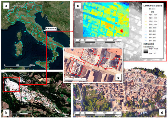
Figure 1.
(a) Amatrice location (Central Italy); (b) WorldView-3 image (Amatrice inner city within the red box); (c) Example of LiDAR Point Cloud coverage and derived DSM; (d) Amatrice inner city post-event 3-D rendering (DSM derived from LiDAR Point Cloud and orthophotos textures); (e) Example of rubble heap delimitation within Amatrice.
The consequences of such a long series of seismic events is that building collapse can occur several days after being seriously damaged by the most intense earthquakes.
3. Materials and Methods
3.1. Dataset
The following territorial data and information were used:
- a WorldView-3 (WV3) Very High Resolution (VHR) satellite frame (1.35 m above ground resolution—a.g.r.—for the 8 (VIS-NIR) multispectral channels; 0.33 m a.g.r. for panchromatic channel) acquired on 08/25/2016, after the first seismic event in Amatrice;
- hyperspectral signatures of the main urban constituents of the seismic rubble acquired, through an ASD-FieldSpec Pro hand-held radiometer, on rubble piles of test areas located in the centre of Amatrice, during a specifically designed survey carried out in December 2016. The hyperspectral signatures (2300 narrow bands, wavelength between 350–2500 nm. 1.4–2 nm as FWHM: Full-Width-Half-Maximum) were acquired by placing the ASD probe perpendicularly at distance of about 0.25 m from the surface of the different rubble typologies visually recognized. The 25° FOV provided by optic accessory allowed us to capture the reflectance from a circular surface area with about 11 cm of radius. These hyperspectral signatures were used in the adopted SMA approach to better deal with the spectral and spatial heterogeneity of the urban rubble, typically smaller than the WV3 pixel;
- two hyperspectral signatures of uncoloured typical cover (grey-looking, similar to concrete) containing asbestos, at different aging levels, involving colonization by typical micro flora of roofs additionally introduced from literature [42], as significantly representative of those dangerous materials likely present in seismic rubble;
- 1 m pixel Digital Terrain Model (DTM) derived from LiDAR data acquired during 2016 flight and RGB orthophotos (0.15 m ground spatial resolution, 2016 flight) for satellite images geometric orthocorrection;
3.2. Data Processing
The whole methodology was developed according to the general scheme depicted in Figure 2 and described in the following paragraphs. The left side of Figure 2 (dashed box), regarding the procedures for retrieving the rubble heaps boundaries and the relative volumes, was actually the objective of a previous work [1]; hence, its description is reported only in the Appendix A, whose objective is to add crucial information regarding the main (surface) constituents of rubble heaps to this geometric information.
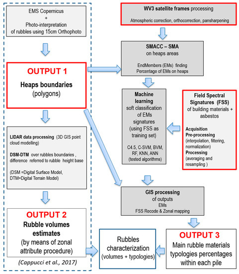
Figure 2.
Flow diagram of the implemented procedure. The input data are: (1) LiDAR point cloud data, RGB aerophotos, Copernicus EMS building damaging grade map; (2) WorldView-3 multispectral data; (3) hyperspectral signature library; (4) polygonal cover and related attributes of rubble heaps, from previously developed procedure [1], in input to SMACC and GIS processing. The rough outline of rubble volume estimates procedure (dashed box) has been included here only for completeness.
3.2.1. Determination of Heap Volume
The rubbles heaps boundaries were basically provided by the Copernicus EMS mapping, furtherly improved (according to our purpose) by visual interpretation of a 15 cm RGB orthophotos photointerpretation. For the volume estimation, Digital Elevation Model of terrain (DTM) and Digital Surface Model (DSM), produced from LiDAR surveys, were exploited: in particular pre-event DTM (DTMpre) and post-event DTM and DSM (DTMpost and DSMpost) were considered.
To each polygon (i.e., heap boundary) the building’s base elevation value was manually assigned, deriving it from the DTMpost in correspondence with a visible point (e.g., portion of the surrounding streets free of rubbles), identified close to the considered rubble. The volume of a single rubble heap was estimated as the solid (3-D space) included between the bottom surface represented by the building’s foundation developing at a constant altitude and the upper uneven surface represented by the DSMpost values over the polygonal area itself. In other words, the volume is assessed through the difference between the DSMpost and the DTMpost values (constant altitude) over the area identified by the heap’s perimeter. An alternative approach has made it possible to perform the assignment of the elevation values of rubble’s base automatically. The base values are automatically extracted by the pre-event DTMpre, which can be assumed as the bottom surface. Therefore, the volume calculation is directly obtained by the difference in elevation between post-event DSMpost and pre-event (DTMpre over the rubbles’ perimeter). For further information about volume heap calculation of Cappucci et al. [1], see Appendix A.
3.2.2. In Situ Data Collection and Pre-Processing
The hyperspectral signatures of rubble materials were collected during a field survey carried out on the 6th and 7th of December 2016. Up to 150 hyperspectral signatures (each made up of about 2300 spectral narrow bands) were acquired. Most of them referred to the five principal building materials (rubble debris, concrete, tiles, bricks, natural stones) and the others to secondary/accessory materials (i.e., zinc/copper gutter, bitumen sheath). It is worth noting that the spectral signatures of the five principal building materials differed significantly among the various piles/urban places. Consequently, after the usual pre-processing (interpolation in the water vapor absorption bands, filtering and normalization in case of calibration faults), for each of the main five building materials, four different averaged signatures were worked out and stored in the spectral library. Therefore, the spectral library resulting from the in situ measurements included eight macro-classes (the abovementioned five main building materials plus the three accessory materials), characterized by twenty-three averaged signatures, with twenty (5 × 4) related to the main five building constituents and three to the accessory materials).
Additionally, two hyperspectral signatures of differently aged and colonized (by vegetal species) asbestos building materials were retrieved from the literature and included in the library, in order to test the possibility of also detecting this dangerous material through satellite data [42]. Therefore, in the end 25 hyperspectral signatures distributed into 9 macro-classes (considering one asbestos macro-class subdivided into the two different aging stages) were finally available.
To make these hyperspectral signatures compatible with the spectral configuration of the WV3 sensor, they were resampled using the related band spectral filters functions. The satellite sensors use electronic band-pass filters to achieve the different spectral band responses from the broad spectrum captured signal. Their analytic expression filter functions, indicated as fij, (i, j indicating, respectively, wavelength and band) and ranging between 0 and 1, can be used to derive the multispectral signatures from the hyperspectral ones by convolving them as follows:
where bj stands for multispectral response in band j, fij is the filter function of j band of satellite sensor (available from the data provider) and Ri the hyperspectral reflectance data. In this context, this resampling step is mandatory to make the in situ hyperspectral signatures compatible with the multispectral ones derivable from the WV3 data.
3.2.3. Satellite Data
Acquisition and pre-processing (geometric, radiometric and atmospheric corrections) of VHR satellite remotely sensed and auxiliary data.
The geometric pre-processing and the orthocorrection of WV3 frames were accomplished using suitable DEM and the rational polynomial coefficients (RPC) provided with the WV3 files with the support of detailed cartography in the WGS 84 / UTM zone 33N projection [43].
In general, satellite imagery is affected by light-wave scattering and attenuation from air molecules, haze, water vapor and particulates, depending on atmospheric turbidity. These noise factors may be present in any given scene and they are typically not uniformly distributed. Given the thickness of the atmosphere crossed by the satellite signals coming from earth surface, the degrading effects introduced may be relevant in many cases, even in some cases making remotely sensed imagery unusable. In our case, aiming at exploiting the field hyperspectral reflectance of specific building materials, the removal of atmospheric effects from satellite imagery is necessary in order to retrieve the corresponding reflectance at ground level. To this end we used the FLAASH (Fast Line-of-sight Atmospheric Analysis of Hypercubes) code, integrated in L3HARRIS Geospatial ENVI® image analysis software, which allows the automatic retrieval of aerosol optical thickness on processed frames using well established algorithms [44,45]. It is worth noting that among the two options we tested—atmospherically correcting the WV3 images first and then performing pansharpening versus first performing the pansharpening and then the atmospheric correction—the latter provided the better results when checked visually.
Moreover, in order to improve the geometric accuracy of the final results, the panchromatic data provided by WV3 sensor at 0.33 m a.g.r. were exploited using the Gram-Schmidt pansharpening method. This choice represented a compromise to preserve both spectral and spatial information, so as to improve the geometric accuracy of final results [46]. Although its performances for spectral features are not at top, it was selected on the basis of preliminary visual interpretation of the results obtained using atmospherically corrected data [47]. In addition, considering that our interest was in improving spatial resolution and that the quality assessment of pansharpened images is still an open issue, the selection was determined also by easy to use and robust implementation of the algorithm within the most diffuse packages for satellite remotely sensed data processing [46,47].
In general, the pansharpening and atmospheric pre-processing of satellite data are performed to improve the results of subsequent classification (based on categorical labelling approach) or regression (based on continuous variables modelling) processes. Few authors have dealt with the evaluation of the suitability of the sequence in performing these two pre-processing steps (commutability) for these two different needs [48]. However, in agreement with the approach adopted here, it was reported that performing the atmospheric correction after the pansharpening, provides better results in continuous modelling approaches, [49].
3.2.4. SMA-SMACC
Data provided by the abovementioned multispectral synthetic image were used as input to the SMA procedure. Indeed, the composite nature of remotely sensed spectral information often hampers the detailed identification and mapping of targeted constituents of the earth’s surface. SMA is a well-established and effective technique to address this spectral mixture problem. SMA models the pixel mixed spectrum as a linear or nonlinear combination of its constituent spectral components (or spectral endmembers) weighted by their subpixel fractional cover. By model inversion SMA provides subpixel endmember fractions [50]. SMA models can be classified into linear and nonlinear ones, depending on the way they model the complexity of light scattering in the spectral mixture analysis. In this paper, we consider linear spectral mixtures, which is considered more effective in the case of an absence of interaction between the component responses, and which may be expressed as:
where:
- Y(i,k) = ith pixel spectral response in kth spectral band;
- Xj(i,k) = ith pixel spectral response of jth endmember in kth spectral band;
- fj(i) = pixel fractional abundance of jth endmember;
- v(i,k) = pixel residual noise in the kth band;
with as basic constraint to fractional pixel reflectance contributions.
In the Equation (2), Xj(i,k) indicates the spectral signature of the jth endmember, Y(i,k) is pixel reflectance response, found through SMACC algorithm by applying consecutively the maximum convex cone constraint. The algorithm also assesses the related fractional abundance fj(i) by minimizing the residual term v(i,k). In the case of an a priori fixed number of endmembers, usually the constraint is assumed to improve the effectiveness of the algorithms by introducing also a shadow endmember. This latter includes the remaining of reflectance contribution to unity, arising for example from possible different illumination condition of the endmember portions within the pixel. Assuming the shadow endmember includes proportionally all the less illuminated parts of all others, estimated through SMA, their preventive normalization at pixel level is required, using their sum as normalization factor.
To retrieve the endmembers, the SMACC algorithm selects the extreme points at borders of the multidimensional distribution of pixels’ spectral signatures establishing a convex cone delimited by the related extreme pixel spectral vectors (endmember spectral signatures), which are located and used as spectral endmembers. The algorithm starts with a single endmember with maximum albedo and incrementally increases their number using the oblique projection that maximize angle between the previous set of pixel extreme vectors to find the subsequent endmember. The cone grows by encompassing the new endmembers, and the iterative procedure repeats until an endmember is found that is already contained within the convex cone, or until the user-defined maximum number of endmembers has been reached. The convex cone formed by extreme vectors or endmembers contains the remaining data vectors that can be modelled by a linear combination of endmembers with the positive coefficients being identified as abundances of the endmembers. It is worth noting that the number of endmembers can ideally exceed that of used spectral channels of the sensor. This is a very useful feature especially when we deal with multispectral data having a limited number of reflectance bands. However, their number should be maintained at a similar level, even when a limited endmembers basis may represent/guarantee just a coarse approximation of the many materials and their spectral variations found in seismic rubble, in order to ensure that a well-conditioned and linearly independent model is obtained. In fact, endmember extraction from hyper/multispectral data remains a challenge task, considering the within-class spectral reflectance variance and noise contributions from various factors (sensor, atmosphere, illumination) to the endmember signatures. Sometimes an endmember may characterize a mixture of materials having very similar spectral signatures rather than represents a single material. More endmembers than pure covers are often retrieved in a remotely sensed imagery and frequently some of them, less important for scene description, can be coalesced in the above introduced shadow endmember.
The SMA through SMACC was performed on the data from the 8-band multilayer at 0.3 m. of a.g.r., obtained from WV3 pansharpening and atmospheric correction processes, considering only the pixels belonging to the identified rubble heaps. The area investigated through SMA corresponds with pixels belonging to the identified rubble heaps furtherly reduced by excluding those pixels whose vegetation cover was too relevant (e.g., rubbles spread on tree-covered scarps). This was achieved by selecting only pixels whose Normalised Difference Vegetation Index (NDVI) values were below a suitable threshold.
Taking into account the number of available bands and the number of the materials to be discriminated, the number of endmembers to be worked out by SMA was fixed at 10 (plus shadow), being aware that a small excess may be tolerated by the method without compromising its robustness too much. In addition, the SMA algorithms provided the percentage of these endmembers for each pixel within the heap surface.
3.2.5. Machine Learning
Then we adopted a supervised classification schema based on various machine learning algorithms, using the 25 resampled spectral signatures of the materials included in the (spectral) library as a training set in order to link these spectral signatures to the endmembers retrieved by SMACC. It is worth underlining that the association of the retrieved endmembers with the signatures of rubble materials acquired on field was rather complex, due to both the above-cited noise factors affecting remotely sensed techniques and the intrinsic spectral variability of field data, characterized indeed by multiple signatures for the same building material. Six typical machine learning algorithms were preliminarily selected for supervised classification of endmembers, taking into account their different capabilities and performance in various situation of noise, limited class samples and outlier presence in input data. The selected algorithms were: C4.5 (decision tree), C-SVC (Core Support Vector Machine—discrete class, continuous input), BVM (Ball Vector Machine), KNN (K-nearest neighbours), RF (Random Forest), ANN (Artificial Neural Network). The latter, though, preliminarily provided very poor results, so it was not considered anymore in the processing chain.
C4.5 makes it possible to implement easy-to-interpret classification models by hierarchically splitting the training data set. This algorithm selects the best subset of attributes based on an entropy measure and organizes the classes in a decision tree rule-based structure. Each node of the tree relates to a split in the feature space, which is always orthogonal to its axes [50,51,52]. C-SVC, more often used in the per-pixel classification context, is a non-parametric supervised statistical learning technique with robustness against outliers and limited train. It is able to estimate a hyperplane in the feature space that minimizes misclassifications [41,52]. BVM is an improvement of standard SVM algorithm which combines techniques from computational geometry based on hyper-spheres to efficiently achieve a close-to-optimal solution [53]. The K-nearest neighbour algorithm (KNN) is a method for classifying objects based on the closest training examples in an n-dimensional feature space. Given an unknown feature pattern, the classifier searches the pattern space for the k training tuples that are closest to the unknown one [53]. The ANN nonparametric algorithms are based on the neural network concepts and work without assumptions about input data distribution and independency. They learn from the training dataset and build relationships (networks) between input (features) and output nodes (classes) through hidden neurons layer connection weights modulation. In our context, a critical issue for ANN effectiveness may be the amount of training occurrences [41]. The Random Forest classifier consists of a group of decision trees induced with different sub-sets of the training data. Each tree of the forest casts a vote for the class to which a given analysis unit (in this case, a given segment) should be associated. The class with most votes is the one associated with the segment [41,54].
These machine learning algorithms were tested as classifiers of endmembers with the objective of evaluating their capability to discriminate as much as possible among the 25 materials present in the library including asbestos. The selection was performed on the basis of error rate minimization in recognizing the classes of training set coupled with the assignment of the maximum number of main materials to endmembers.
3.2.6. Accuracy Assessment
The accuracy assessment of the thematic maps obtained from the usual hard classification scheme is a mandatory step to be accomplished using randomly selected samples, where the categorical class assignment provided by the classifier algorithm is verified through independent observations. However, this approach was not directly applicable to the results of SMACC SMA analysis, which provide continuous distributions of endmembers abundances within each pixel. Therefore, an original approach that also allowed us to assess accuracy for SMA-derived endmember abundance distributions was implemented. To this end, only the pixels where one endmember predominates the others and its abundance is superior to a predefined threshold were selected to be considered quasi pure in a spectral sense. To this end the pixel Predominant Endmember class Distribution (PED) was obtained by the maximum abundance distribution (PMA), in turn derived from the endmember distributions using different thresholds to exclude the pixels with lower PMA values. This allowed us to transform the multilayer of endmember abundances continuous distributions into a categorical distribution of predominant endmember classes (PED) to which a classical accuracy assessment scheme was applied.
Thus, the accuracy of the PED obtained from the results of the SMACC SMA, using the 0.3 m pan-sharpened WV3 data, was tested using a photointerpretation approach of random point samples reported on the RGB aero-photos (0.25 m a.g.r.), supported by preliminary unsupervised clustering analysis. To facilitate the photointerpretation approach, the five macro-classes of main rubble materials (Table 1) were grouped into three more visually discriminable categories:

Table 1.
Considered urban rubble constituents.
- 1st—debris-concrete (characterized by light grey shades);
- 2nd—tiles-bricks (characterized by reddish shades);
- 3rd—natural stone (characterized by dark grey shades).
Accordingly, the PED was recoded on the three previous groups (categories) through the classification output obtained by the machine learning algorithm to produce a three classes thematic map of the predominant endmembers. Then, the accuracy of this former was estimated using a randomly selected point sample whose classes were independently derived by means of photointerpretation on the corresponding RGB aero-photos. However, it is worth noting that excluding the few pixels exploited for deriving the SMACC endmembers (statistically insufficient for an effective accuracy assessment), most of rubble pixels are a mix of the three categories previously introduced. At the pixel level, the predominant (maximum abundance) endmembers are characterized by different abundances less than 1. In particular, the first category (debris-concrete) was prevalent in the majority of pixels and showed the highest sensible abundance values with respect to the other two classes.
Generally, the endmember maximum abundance values of the others two classes were lower, and these classes were prevalent in a minor number of pixels. Of course, greater is the abundance of the specific category in the pixel and more effective is the photointerpretation and consequent labelling. Therefore, increasingly rising abundance threshold values were adopted in order to provide a statistically sufficient number of samples for all three of the classes introduced above.
Accordingly, three related confusion matrices, one for each selected abundance threshold, were calculated, showing different overall accuracies and k-statistics parameters. Then, using the classification of the endmembers into the 25 classes of the library provided by machine learning classifiers, the percentage distribution of these classes was worked out.
3.2.7. GIS Processing
Finally, the characterization of rubbles within the test area was obtained through zonal GIS processing of the heaps’ polygonal cover. In particular, for each heap, the mean values of the fractional abundancies of the three main constituents were assessed. Of course, by multiplying each average value by the number of pixels of the heaps, the surface percentage of the corresponding (surface) materials abundancy, at heap level, is calculated.
4. Results
Eight principal constituents (macro-classes) of urban rubble were identified in the field during the two-day survey, during which 150 hyperspectral signatures (about 2300 narrow bands for each spectral signature) were acquired. In Table 1, the nine related macro-classes, including the asbestos macro-class, whose spectral signatures were derived from the literature, are reported.
The majority of these field data refer to the more abundant rubble materials, which correspond to the first five macro-classes, whose spectral signatures differed significantly among the various piles and urban places. Therefore, after a preliminary analysis and in order to preserve the spectral variability of these five materials, four different averaged signatures were recorded for each of them.
In Figure 3, the four graphs show: the in situ hyperspectral signatures acquired on concrete (top left graph) and brick (top right graph) after the first pre-processing phase but before smoothing by filtering; the corresponding filtered spectral signatures of the concrete (lower left graph) and brick lower right graph) categories. The bottom image of Figure 3 represents some samples of the eight types of rubble materials.
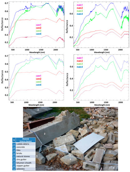
Figure 3.
In situ hyperspectral signatures of concrete (top left) and brick (top right) after the first pre-processing phase but before smoothing by filtering and corresponding filtered spectral signatures of the concrete (lower left) and brick (lower right) categories. In the bottom image some samples of the eight types of rubble materials (white numbers to be matched with the legend on the left lower corner of the image) are displayed.
The graph in the upper part of Figure 4 shows the multispectral signatures resampled using the WV3 sensor filter function (the asbestos signatures were omitted for clearness). The multispectral signatures of the 10 endmembers, extracted via SMACC from WV3 data of rubble heaps, are reported in the lower graph of Figure 4.
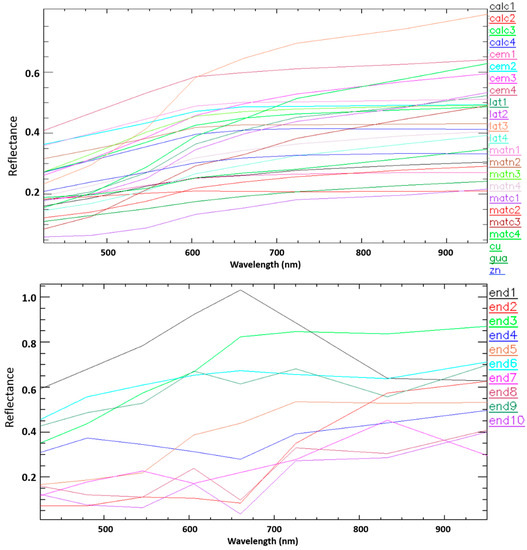
Figure 4.
Resampled multispectral signatures of the 23 in situ rubble materials (upper graph); Multispectral signatures of endmembers extracts using SMACC algorithm (lower graph).
From the WV3 pansharpened pre-processed imagery a small number (10) of pure material signatures, i.e., endmembers, were derived through the SMACC algorithm to be used as reference for the main material classes of urban rubble, by matching them with the resampled multispectral signatures of the in situ materials using machine learning classifiers. The SMACC algorithm thus provided a multilayer distribution of ten endmembers, plus shadow, whose basic statistics are shown in Table 2.
Table 2.
Basic statistics for the EMs abundance distribution of WV3 pansharpened data.
The first five endmembers except end3, plus shadow, are the most abundant, on average, as reported in Table 2. In particular, the shadow shows high abundance values in a relevant number of pixels, as shown in Figure 5, where the distributions of the abundance of the shadow and first five endmembers are depicted.
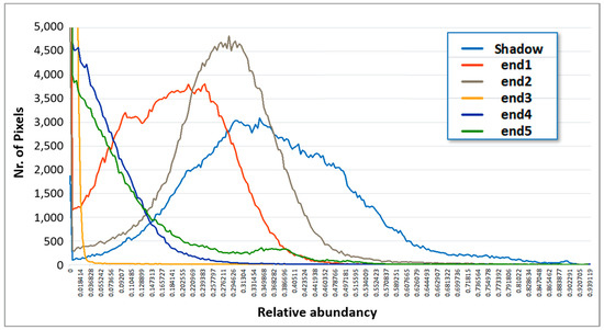
Figure 5.
Histogram distribution of the first EM abundances including shadow.
After the spectral resampling, each of the 25 resampled signatures, corresponding to one of the nine main macro-classes of urban rubble materials identified on field, was matched (classified) with those of EMs derived from the WV3 pansharpened data using several machine learning algorithms. The related results are reported in Table 3. Please note that the x suffix, x = 1 to 4, in the first five class labels and x = 1 to 2 in the asbestos labels, refers to the four averaged signatures stored in the library for each of the five main rubble materials and to the two signatures available for asbestos, respectively. In the first 25 rows of Table 3, the train classes corresponding to the 25 spectral signatures stored in the library (“Training” column) and the related class labels assigned by the exploited classifiers (3rd to 7th column) are reported, respectively.
Table 3.
The results obtained with different machine learning algorithms for endmember-supervised classification to assign the rubble typology labels to them, are reported in the last 10 rows of table (in light grey and darker grey for C-SVC, exploited in the subsequent steps). The first 25 rows show the training results for the different machine learning algorithms tested: BVM, C-SVC, KNN, RF, C4.5. The error rate in training was reported under the column label indicating the algorithm.
Moreover, in the first row of Table 3, beneath each classifier label, the related error rates (number of wrong classified samples/total number of samples) achieved are reported, indicating C-SVC and RF as the best performing algorithms (minimum error rate; note that RF’s 100% suitability against the training set is a priori guaranteed by definition). In the remaining row, the classification of the ten endmembers (end1÷end10), by means of each classifier, are shown.
Since the C-SVC algorithm is recognized to be robust against a poor training set and it was able to discriminate one main class more (i.e., the natural stone) than the RF, these classification results were selected to assess the distribution of the main materials. Instead, the results of RF were exploited to detect the presence of asbestos. Starting from the multilayer of endmembers abundance, the predominant endmember distribution (PED), for the three main grouped categories defined for the accuracy assessment, was derived through that of pixel maximum abundance (PMA) using suitable thresholds.
As shown in Figure 6, the abundance of the first macro-class (concrete-rubble debris) is prevalent in a large number of pixels (see Figure 6b—PED) and shows the highest values (as shown in Figure 6a—PMA), while those of the other two macro-classes are lower in value and prevalent in a minor number of pixels.
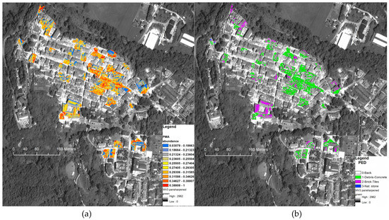
Figure 6.
(a) Pixel Maximum Abundance (PMA) and (b) Predominant Endmember Distribution (PED) displayed on a grey level background (pansharpened red).
Taking into account the abovementioned results, the PED categorical distributions corresponding to different minimum PMA thresholds (0.25, 0.35 and 0.45), selected on the basis of the PMA’s histogram (Figure 7), were calculated to be used for the accuracy assessment. In this way the three rightmost fractions of the histogram distribution (Figure 7) were selected to generate the maps whose accuracy was assessed.
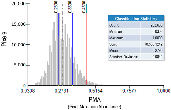
Figure 7.
Histogram distribution of PMA with thresholds exploited for accuracy assessment.
In Figure 8 the recoded PED distribution obtained using a 0.25 PMA threshold is displayed.
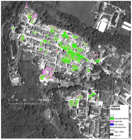
Figure 8.
Recoded PED distribution map of the three main categories at 0.25 PAM threshold.
The accuracy assessment was then performed by comparing the PED classes at randomly selected points with the classes independently derived (for the same points) by photointerpretation. The accuracy assessment results obtained using the three thresholds for PMA, are reported in the following confusion matrices with the related accuracy parameters (Table 4, Table 5 and Table 6).
Table 4.
Confusion matrices for the recoded PED maps obtained using the 0.25 PMA threshold (461 samples).
Table 5.
Accuracy parameters of three recoded PED maps obtained using the 0.35 PMA threshold (477 samples).
Table 6.
Accuracy parameters of three recoded PED maps obtained using the 0.45 PMA threshold (252 samples).
The random sample was about 1–2% of the entire population, being at its maximum when the 0.25 threshold was used and decreasing sensibly with the threshold rise (Figure 6). However, it must be underlined that the samples number effectively exploited for 0.25 PMA threshold is lower than that related to the 0.35 one, due to the exclusion of samples found contaminated by vegetation.
According to the RF classification results, endmembers n. 5 (proxy of the asbestos’ distribution) was worked out and reported in Figure 9. The different colours represent the asbestos relative abundance on rubble heaps.
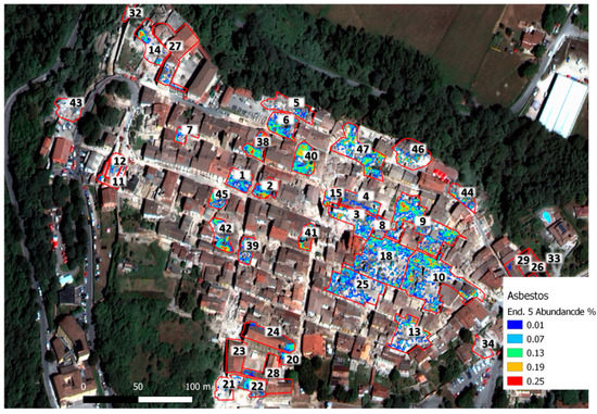
Figure 9.
Asbestos distribution on rubble heaps with black labels and red borders. Background: pan-sharpened true colour.
It must be highlighted that, probably due to misclassification of aged dark-red tiles erroneously assigned to worn asbestos, which is also caused by diffuse colonization of local roofs by micro flora, the asbestos distribution initially showed unlikely highest concentrations (abundance > 0.3) corresponding to intact tile roofs (rubble heaps n. 23–26, 27–29). Therefore, after a visual analysis, a maximum accepted value of 0.25 was applied to avoid this overestimate, providing a more realistic distribution of asbestos within rubble. Then, as shown in Figure 10, the n. 2, 4, 8, 9, 10, 42 heaps are those characterized by areas with the highest asbestos’ concentrations.
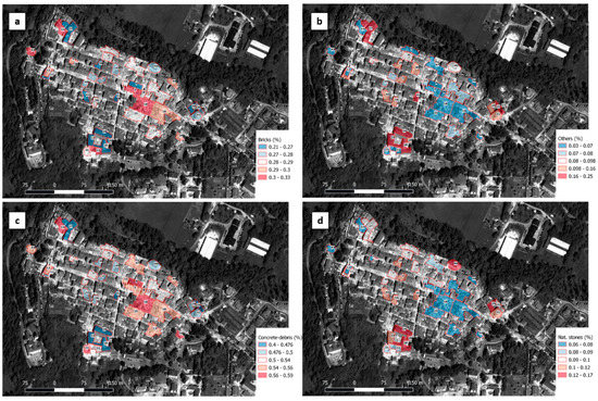
Figure 10.
Estimated percentage distributions of the types of materials found within the rubble heaps in the centre of Amatrice town. The four maps refer respectively to: bricks (a), other building materials (b), concrete-debris (c) and natural stone (d).
Finally, the zonal processing of the raster map derived from the classification implementing the per pixel distribution of endmembers percentages, provided us with the relative percentages of the three main categories used for the accuracy assessment within the rubble heaps. The estimated distributions of the main materials’ typologies are shown in Figure 9. The most abundant rubble heap typology (macro class) is represented by concrete/debris (range: 40–50%), followed by brick/tiles (range: 25–30%) and natural stones (range: 7–17%), with other materials (metal, plastic, bitumen sheath, etc.) deriving from the remaining endmembers completing the list (range: 3–25%).
In Table 7 an example of the quantitative results provided by the whole procedure is reported for several rubble heaps. Indeed, for each heap the procedure makes it possible to determine the volume and the main constituents’ percentages, including the information regarding the presence of asbestos.
Table 7.
Volumes and main constituents (for a sample of rubble heaps located in the most affected area). For each heap the asbestos’ presence is also indicated.
5. Discussion
The selection and exploitation of machine learning algorithms for matching (classifying) the SMACC endmembers’ spectral signatures to those derived from the field hyperspectral signatures was an important and critical step of the work.
The global assessment of the algorithms’ performance was accomplished taking into account both the right classification of training materials, summarized by the related error rate (Table 3), and the number/typology of main materials (including asbestos) detected through the endmembers.
The endmembers labelled by BVM classifier accounted for the four main materials (cem, matc, lat, matn) plus gua (see Table 3), but failed to discriminate the training samples. In addition, the results showed an unreliable assignment of the asbestos class. Conversely, the C-SVC performed the best with regard to training sample classification, and was also able to associate the four endmembers with the four main materials. Although the KNN performance in classifying the training set was slightly better than that of BVM, it wasn’t able to avoid unrealistic asbestos labelling for the three training samples with respect to other rubble materials. However, this algorithm was able to account for four main rubble materials through the endmembers so as the RF. The latter was, in particular, the only one able to detect the likely presence of asbestos (end5). The related endmember (n. 5) showed an average abundance of few percent but with the highest standard deviation meaning a significant concentration of this dangerous material in specific heaps (Table 5). Finally, the C4.5 was the worst performing, both in classifying the training set and in the number of main materials associated with endmembers.
Following these criteria, the C-SVC and RF were the best performing. Moreover, these two algorithms agreed with the labelling of the five endmembers. They were able to discriminate four main materials with differences in terms of natural stones (matn), which was detected by C-SVC but not by RF, which instead was able to classify rubble debris (calc), which was missed by the other classifier. Therefore, the ten endmembers provided by the SMA from pansharpened WV3 data were satisfyingly mapped to the in situ spectral signatures of the rubble materials using C-SVC machine learning algorithm, which made it possible to obtain the most effective discrimination of the main building materials (first 5 endmembers of Table 1).
In agreement with the general schema of the mapping model, which includes validation and accuracy assessment based on independent measurements, an original method for accomplishing this necessary test on the obtained continuous distribution of rubble typologies was implemented. It is based on the pixel maximum abundance (PMA) and predominant endmember (PED) distributions, derived from the SMA outputs. The PMA histogram distribution (Figure 6) confirms once again the extreme spectral heterogeneity of rubble, with a maximum of less than 0.3. Such an approach allowed us to assess various PED distributions (obtained using different PMA thresholds) using photointerpretation method, i.e., by comparing corresponding locations on the RGB high-resolution aerophotos. According to the typical thematic accuracy assessment it was possible to evaluate overall accuracy (O.A.) and K parameters through related confusion matrices. As expected, the overall accuracy (O.A.) assessed for the three PMA rising thresholds (Table 4, Table 5 and Table 6) increases with the threshold increase due to endmember predominance increasing at pixel level, which in turn makes correct photointerpretation easier. Indeed, both O.A. and K accuracy global parameters are maximum (i.e., 0.888 and 0.754, respectively) at the 0.45 threshold, which is in substantial agreement with the photointerpretation results. Although this relative abundance value is low, it seems sufficient to allow the pixel main material to be recognized by the independent expert interpreter.
Additionally, the PED maps obtained with the two lowest thresholds (0.35 and 0.25) correspond to a poorer/moderate agreement with the photointerpretation according to the decrease in endmember predominance [55].
The classification of materials present on the surface of rubble heaps is one of the most important results achieved in the present study. Among these, asbestos is of great interest due to its implications for human health (for both earthquake survivor population and rescue teams). The present work showed that concrete debris and brick tiles are more abundant (Table 7 and Figure 11a) within the study area and about 50% of the rubble heaps may contain asbestos (in different quantities; Table 7 and Figure 11b).
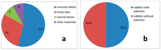
It does not mean that 50% of rubbles contains asbestos in concentrations that could be harmful to human health. However, the present research demonstrate that it is possible to identify the potential presence of this hazardous substance and support management of waste and rubbles to be removed. Sustainable land reclamation is one of the main goals of ENEA as it has a great socioeconomic importance with a high impact on economic development [56]. Results of the present study are of extreme practical and logistical relevance, and it could be replicated to improve the effectiveness of management in post-earthquake emergencies around the world.
6. Conclusions
The radiometric and geometric resolution parameters of the remote sensors play an important role in allowing suitable mapping of the spectral-spatial heterogeneity typical of urban and industrial/infrastructure areas. In particular, they are fundamental for the discrimination of the seismic rubble at the required scale. To achieve this goal, the panchromatic and multispectral information provided by WV3 sensors were fused using the Gram-Schmidt pansharpening method. Subsequently, they were atmospherically corrected in order to obtain a suitable input at 31 cm of a.g.r. for the SMA procedure. In general, even though widely exploited for their improved geometric resolution, the quantitative use of synthetic spectral reflectance of pansharpened products is not widespread, since the degradation of the quality during the fusing processes does not make it possible to fully preserve the original spectral properties of the acquisition channels. In this case, rather effective results were obtained by performing the pansharpening process using the spectrally conservative Gram-Schmidt method prior to atmospheric correction. The inverse procedure (atmospheric correction carried out before pansharpening process) did not produce the quality level in the results.
The implemented methodology provided the relative abundance distribution of the considered rubble materials. The results are in agreement with the information that has been made available until now with respect to transportation and final disposal. Indeed, concrete and rubble debris were the most abundant seismic rubble typologies. These findings are consistent with the typical proportion of building materials within the centre of Amatrice and the propensity of debris to spread over heaps surface in case of building collapses (Figure 7, Figure 9). The clean-up and removal of rubble has not yet been completed in the central Apennines, and relevant information obtained in the future will be useful for refining the implemented methodology. For instance, one of the crucial feedbacks will be the correspondence between the material distribution retrieved at the surface and the inner part of the rubble heap.
Although detailed information about the asbestos distribution over rubble heaps was not available, the global presence of this dangerous material, mainly as a constituent of roof covers, has been reported by various independent observations made in the field and by transportation operators in charge of clearing the rubble from the centre of Amatrice. In this context, it was not possible to test the accuracy of the asbestos distribution retrieved through RF machine learning algorithm.
In the context of post-event activities related to seismic events, the effective management of the huge amount of resulting rubble and debris in urban areas represents one of the major issues and can be usefully supported by EO-based monitoring and mapping applications, also exploiting the last generation of multispectral satellite VHR sensors. The surveys from the aerial platform can provide detailed up-to-date information, but are extremely expensive for the continuous monitoring of emergency areas required for controlling the evolution of the earthquake urban scenario, which instead can be repetitively mapped by available sensors on board orbiting satellite platforms, which can provide an increasing amount of territorial data with continuously improving spatial and spectral resolution. Results obtained at the present time through the innovative methodology developed in this work show the applicability of the WV3 satellite VHR data for providing effective surface estimates of the distribution of seismic rubble types in heaps distributed within urban areas. This information can be advantageously integrated with that from related volumes derived from aerial surveys carried out in the aftermath of the earthquake (Table 2 and Table 7; Figure 8 and Figure 10), providing suitably support to the management activities related to the urban rubble. The stereoscopic acquisition capabilities of VHR satellite sensors could also support the estimation of volumes in monitoring the evolution of the emergency scenario, possibly with a “one-off” calibration based on the LiDAR information deriving from an initial aerial survey. The preliminary analysis of rubble heaps with EO tools can also have a relevant impact on cost of post emergency action like rubble management and the definition of priority in order to guarantee human health protection.
Thus, this original EO-based methodology allowed us to produce realistic estimates of the types and volumes of seismic rubble in the historical centre of Amatrice. It can be generalized with a high degree of automation and can be easily applied to similar situations, even with possible improvements deriving from the integration of the SAR (Synthetic Aperture Radar) and hyperspectral data provided by ongoing EO missions (Copernicus Sentinel-1, Cosmo SkyMed, PRISMA, EnMap). Future activities will include a greater exploitation of high-resolution and hyperspectral satellite data, for assessing both volumes and typologies of earthquake rubble heaps, also investigating the possibility to detect hazardous rubble materials (i.e., asbestos).
Author Contributions
Conceptualization: Flavio Borfecchia, Sergio Cappucci, Ludovica Giordano and Maurizio Pollino; methodology: Flavio Borfecchia, Ludovica Giordano and Maurizio Pollino; formal analysis; Flavio Borfecchia, Ludovica Giordano, Maurizio Pollino; field work activity: Flavio Borfecchia, Sergio Cappucci, Danilo Bersan, Domenico Iantosca; data curation: writing and editing the original manuscript: Flavio Borfecchia, Luigi De Cecco, Ludovica Giordano, Maurizio Pollino, Vittorio Rosato. Sergio Cappucci, while all authors contributed to its review; visualization: Ludovica Giordano and Flavio Borfecchia; supervision: Maurizio Pollino and Flavio Borfecchia; project administration: Vittorio Rosato; funding acquisition: Sergio Cappucci. All authors have read and agreed to the published version of the manuscript.
Funding
The present research has been funded by ENEA and requested by Italian National Civil Protection Department (DPC) under the “Rubbles Agreement”.
Acknowledgments
EO data were provided under COPERNICUS by European Union and ESA. Thanks to F. Campopiano, P. Marsan, P. Pagliara and I. Postiglione of National Civil Protection for the fruitful discussion and suggestions and to all staff involved during the emergency action. The work presented in the paper has been conducted also in the framework of EISAC.it (www.eisac.it), a joint ENEA and INGV collaboration agreement. EISAC.it is an international initiative aiming at establishing a collaborative, European-wide platform, for supporting Operators and Public Authorities in better protecting assets and in enhancing their resilience with respect to all hazards.
Conflicts of Interest
The authors declare no conflict of interest. ENEA is not responsible for any use, even partial, of the contents of this document by third parties and any damage caused to third parties resulting from its use. The data contained in this document is the property of ENEA.
Appendix A
Method 1
The implemented methodological approach, outlined in the left side of Figure 2, is structured into the following steps:
- The collapsed buildings (rubble heaps perimeters) were delimited by means of visual photo-interpretation, taking advantage of orthophotos’ high resolution (15 cm) as well as using the already available Copernicus EMS data. The polygons (P) were traced considering the displacement caused by the oblique photo acquisition (e.g., by integrating the DTMpost and DSMpost in the assessment). Wherever possible, i.e., when a single building was effectively recognizable as a well-defined single structure, a unique rubble heap was digitized for each single building; a pooled polygon referring to a group of (not distinguishable) buildings was sketched otherwise.
- A suitable classification of “level of damage” has been reported, by assigning specific codes to each polygon: (1) “totally collapsed”; (2) “partially collapsed”, (3) “rubbles piled over a slope”; (4) “uncertainty in defining the level of damage”.
- In addition, a classification of building’s typology was performed (assigning a specific class, e.g., “religious”, “residential”, “educational”, “medical”, etc.), to each polygon, supported by Copernicus EMS data, as well as other web sources like Google Maps.
- To each polygon, the building’s base elevation value (B) was assigned: it was derived from the DTMpost in correspondence of a visible point (e.g., portion of the surrounding streets free of rubbles), identified close to the considered building block/rubble. In case of a significant slope of the streets contiguous to the building block, the minimum altitude value among different possible points nearby the area of interest was selected, to not underestimate the actual elevation of rubble heaps (Figure A1).
- The basis of the previously described steps, the volume of a single rubble heap can be estimated as the solid (3-D space) included between the flat horizontal polygon, i.e., the bottom surface (B) represented by the building’s foundation developing at a constant altitude (selected DTMpost value), and the upper uneven surface represented by the DSMpost values over the polygonal area itself. So, the volume is assessed through the difference between the DSMpost and the selected DTMpost value (constant altitude B) over the area identified by the heap’s perimeter, as expressed by the Formula (1):
This calculation was carried out in GIS environment by means of the ERDAS Imagine “zonal attribute” function (Zonal Statistics to Polygon Attributes: this ERDAS Imagine (by Hexagon Geospatial) operator extracts the zonal statistics of the background image of a vector feature layer and save them as vector attributes), which allows to assign the calculated volume value as an attribute of the corresponding GIS polygon representing the rubble heap (in shapefile format).

Figure A1.
Example of building’s base height retrieving. The elevation is estimated from the lower (visible) point adjacent the rubble heap. For instance, in case 2 the lower elevation (right side) is selected.
Figure A1.
Example of building’s base height retrieving. The elevation is estimated from the lower (visible) point adjacent the rubble heap. For instance, in case 2 the lower elevation (right side) is selected.

Method 2
Method 2 follows the same steps 1 and 2 of M1 but different step 3, since the assignment of the elevation values of rubble’s base is not manually performed. Rather, the base values are automatically extracted by the pre-event DTMpre, which can be assumed as the bottom surface.
Therefore, in M2 processing chain, the volume calculation is directly obtained by the difference in elevation between post-event DSMpost and pre-event (DTMpre over the rubbles’ perimeter (step 3), as described in Equation (2):
The above methodology must be cited as [1].
References
- Cappucci, S.; De Cecco, L.; Gemerei, F.; Giordano, L.; Moretti, L.; Peloso, A.; Pollino, M. Earthquake’s rubble heaps volume evaluation: Expeditious approach through earth observation and geomatics techniques. Lect. Notes Comput. Sci. 2017, 2, 261–277. [Google Scholar] [CrossRef]
- Rathje, E.M.; Adams, B.J. The Role of Remote Sensing in Earthquake Science and Engineering: Opportunities and Challenges. Earthq. Spectra 2008, 24, 471–492. [Google Scholar] [CrossRef]
- Ricci, P.; Verderame, G.M.; Manfredi, G.; Pollino, M.; Borfecchia, F.; De Cecco, L.; Martini, S.; Pascale, C.; Ristoratore, E.; James, V. Seismic Vulnerability Assessment Using Field Survey and Remote Sensing Techniques. In Proceedings of the Computational Science and Its Applications—ICCSA 2011 International Conference, Santander, Spain, 20–23 June 2011; Murgante, B., Gervasi, O., Iglesias, A., Taniar, D., Apduhan, B.O., Eds.; Springer: Berlin/Heidelberg, Germany, 2011; Volume 2, pp. 376–391. [Google Scholar] [CrossRef]
- Pollino, M.; Fattoruso, G.; La Porta, L.; Della Rocca, A.B.; James, V. Collaborative Open Source Geospatial Tools and Maps Supporting the Response Planning to Disastrous Earthquake Events. Future Internet 2012, 4, 451–468. [Google Scholar] [CrossRef]
- Kerle, N. Remote Sensing of Natural Hazards and Disasters. In Encyclopedia of Natural Hazards; Encyclopedia of Earth Sciences Series; Bobrowsky, P.T., Ed.; Springer: Dordrecht, The Netherlands, 2013; pp. 838–847. ISBN 978-90-481-8699-0. [Google Scholar] [CrossRef]
- Borfecchia, F.; De Canio, G.; De Cecco, L.; Giocoli, A.; Grauso, S.; La Porta, L.; Martini, S.; Pollino, M.; Roselli, I.; Zini, A. Mapping the earthquake-induced landslide hazard around the main oil pipeline network of the Agri Valley (Basilicata, southern Italy) by means of two GIS-based modelling approaches. Nat. Hazards 2016, 81, 759. [Google Scholar] [CrossRef]
- Joyce, K.E.; Belliss, S.E.; Samsonov, S.V.; McNeill, S.J.; Glassey, P.J. A review of the status of satellite remote sensing and image processing techniques for mapping natural hazards and disasters. Prog. Phys. Geogr. 2009, 33, 183–207. [Google Scholar] [CrossRef]
- Ricci, P.; Gaudio, C.D.; Verderame, G.; Manfredi, G.; Pollino, M.; Borfecchia, F. Seismic vulnerability assessment at urban scale based on different building stock data sources. In Proceedings of the 2nd International Conference on Vulnerability and Risk Analysis and Management (ICVRAM), Liverpool, UK, 13–16 July 2014; p. 12. [Google Scholar]
- Kader, A.; Jahan, I. A review of the application of remote sensing technologies in earthquake disaster management: Potentialities and challenges. In Proceedings of the International Conference on Disaster Risk Management, Dhaka, Bangladesh, 12–14 January 2019; p. 6. [Google Scholar]
- Ji, M.; Liu, L.; Du, R.; Buchroithner, M.F. Neural Network Features for Detecting Collapsed Buildings after Earthquakes Using Pre- and Post-Event Satellite Imagery. Remote Sens. 2019, 11, 1202. [Google Scholar] [CrossRef]
- Wang, X.; Li, P. Extraction of earthquake-induced collapsed buildings using very high-resolution imagery and airborne LiDAR data. Int. J. Remote Sens. 2015, 36, 2163–2183. [Google Scholar] [CrossRef]
- Hussain, E.; Ural, S.; Kim, K.; Fu, C.-S.; Shan, J. Building Extraction and Rubble Mapping for City Port-au-Prince Post-2010 Earthquake with GeoEye-1 Imagery and LiDAR Data. Photogramm. Eng. Remote Sens. 2011, 77, 1011–1023. [Google Scholar] [CrossRef]
- Available online: https://sentinel.esa.int/web/sentinel/missions/sentinel-2 (accessed on 16 January 2020).
- Available online: https://emergency.copernicus.eu/mapping (accessed on 16 January 2020).
- Ouzounis, G.K.; Soille, P.; Pesaresi, M. Rubble Detection from VHR Aerial Imagery Data Using Differential Morphological Profiles. In Proceedings of the 34th International Symposium Remote Sensing of the Environment, Sydney, Australia, 10–15 April 2011; p. 4. [Google Scholar]
- Modica, G.; Pollino, M.; Lanucara, S.; La Porta, L.; Pellicone, G.; Di Fazio, S.; Fichera, C.R. Land Suitability Evaluation for Agro-forestry: Definition of a Web-Based Multi-Criteria Spatial Decision Support System (MC-SDSS): Preliminary Results. In ICCSA 2016: Lecture Notes in Computer Science; Gervasi, O., Murgante, B., Misra, S., Rocha, A.M., Torre, C.M., Taniar, D., Apduhan, B.O., Stankova, E., Wang, S., Eds.; Springer: Cham, Switzerland, 2016; Volume 9788, pp. 399–413. [Google Scholar] [CrossRef]
- Di Pietro, A.; Lavalle, L.; La Porta, L.; Pollino, M.; Tofani, A.; Rosato, V. Design of DSS for Supporting Preparedness to and Management of Anomalous Situations in Complex Scenarios. In Managing the Complexity of Critical Infrastructures; Studies in Systems, Decision and Control; Setola, R., Rosato, V., Kyriakides, E., Rome, E., Eds.; Springer: Cham, Switzerland, 2016; Volume 90. [Google Scholar]
- EPA (United States Environmental Protection Agency). Household Hazardous Waste Management: A Manual for One-Day Community Collection Programs; EPA530-R-92-026; EPA (United States Environmental Protection Agency): Washington, DC, USA, 1993; p. 78.
- Xie, H.; Luo, X.; Xu, X.; Pan, H.; Tong, X. Automated Subpixel Surface Water Mapping from Heterogeneous Urban Environments Using Landsat 8 OLI Imagery. Remote Sens. 2016, 8, 584. [Google Scholar] [CrossRef]
- He, M.; Zhu, Q.; Du, Z.; Hu, H.; Ding, Y.; Chen, M. A 3D Shape Descriptor Based on Contour Clusters for Damaged Roof Detection Using Airborne LiDAR Point Clouds. Remote Sens. 2016, 8, 189. [Google Scholar] [CrossRef]
- Baiocchi, V.; Dominici, D.; Mormile, M. UAV application in post-seismic environment. Int. Arch. Photogramm. Remote Sens. Spat. Inf. Sci. 2013, 1, W2. [Google Scholar] [CrossRef]
- De Canio, G.; Roselli, I.; Giocoli, A.; Mongelli, M.; Tatì, A.; Pollino, M.; Martini, S.; De Cecco, L.; La Porta, L.; Borfecchia, F. Seismic monitoring of the cathedral of Orvieto: Combining satellite InSAR with in-situ techniques. In Proceedings of the 7th International Conference on Structural Health Monitoring of Intelligent Infrastructure, Torino, Italy, 1–3 July 2015; De Stefano, A., Ed.; Volume 1, pp. 415–425, ISBN 978-1-5108-2107-1. [Google Scholar]
- Ma, Y.; Chen, F.; Liu, J.; He, Y.; Duan, J.; Li, X. An Automatic Procedure for Early Disaster Change Mapping Based on Optical Remote Sensing. Remote Sens. 2016, 8, 272. [Google Scholar] [CrossRef]
- Costanzo, A.; Montuori, A.; Silva, J.P.; Silvestri, M.; Musacchio, M.; Doumaz, F.; Stramondo, S.; Buongiorno, M.F. The Combined Use of Airborne Remote Sensing Techniques within a GIS Environment for the Seismic Vulnerability Assessment of Urban Areas: An Operational Application. Remote Sens. 2016, 8, 146. [Google Scholar] [CrossRef]
- Kawakubo, F.; Morato, R.; Martins, M.; Mataveli, G.; Nepomuceno, P.; Martines, M. Quantification and Analysis of Impervious Surface Area in the Metropolitan Region of São Paulo, Brazil. Remote Sens. 2019, 11, 944. [Google Scholar] [CrossRef]
- Borfecchia, F.; Rosato, V.; Caiaffa, E.; Pollino, M.; De Cecco, L.; La Porta, L.; Ombuen, S.; Barbieri, L.; Benelli, F.; Camerata, F.; et al. Remote Sensing and Data Mining Techniques for Assessing the Urban Fabric Vulnerability to Heat Waves and UHI. Preprints 2016, 2016080202. [Google Scholar] [CrossRef]
- Xie, S.; Duan, J.; Liu, S.; Dai, Q.; Liu, W.; Ma, Y.; Guo, R.; Ma, C. Crowdsourcing Rapid Assessment of Collapsed Buildings Early after the Earthquake Based on Aerial Remote Sensing Image: A Case Study of Yushu Earthquake. Remote Sens. 2016, 8, 759. [Google Scholar] [CrossRef]
- Torres, Y.; Arranz, J.J.; Gaspar-Escribano, J.M.; Haghi, A.; Martinez-Cuevas, S.; Benito, B.; Ojeda, J.C. Integration of LiDAR and multispectral images for exposure and earthquake vulnerability estimation. Application in Lorca, Spain. arXiv 2018, arXiv:1806.11019. [Google Scholar] [CrossRef]
- Borfecchia, F.; De Cecco, L.; Pollino, M.; Lugari, A.; Martini, S.; La Porta, L.; Ristoratore, E.; Pascale, C. Active and passive remote sensing for supporting the evaluation of the urban seismic vulnerability. Ital. J. Remote Sens. 2010, 42, 129–141. [Google Scholar] [CrossRef]
- Krówczyńska, M.; Wilk, E.; Pabjanek, P.; Kycko, M. Hyperspectral Discrimination of Asbestos-Cement Roofing. Geomat. Environ. Eng. 2017, 11, 47–65. [Google Scholar] [CrossRef]
- Tommasini, M.; Bacciottini, A.; Gherardelli, M. A QGIS Tool for Automatically Identifying Asbestos Roofing. ISPRS Int. J. Geo-Inf. 2019, 8, 131. [Google Scholar] [CrossRef]
- Niranjani, K.; Vani, K. Geometrical Endmember Extraction and Linear Spectral Unmixing of Multispectral Image. Int. Sci. Press 2016, 9, 7–15. [Google Scholar]
- Benítez, F.L.; Mena, C.F.; Zurita-Arthos, L. Urban Land Cover Change in Ecologically Fragile Environments: The Case of the Galapagos Islands. Land 2018, 7, 21. [Google Scholar] [CrossRef]
- Taramelli, A.; Valentini, E.; Innocenti, C.; Cappucci, S. FHYL: Field spectral libraries, airborne hyperspectral images and topographic and bathymetric LiDAR data for complex coastal mapping. In Proceedings of the International Geoscience and Remote Sensing Symposium-IGARSS, Melbourne, VIC, Australia, 21–26 July 2013; pp. 2270–2273. [Google Scholar]
- Wu, C. Normalized spectral mixture analysis for monitoring urban composition using ETM+ imagery. Remote Sens. Environ. 2004, 93, 480–492. [Google Scholar] [CrossRef]
- Cappucci, S.; Valentini, E.; Monte, M.D.; Paci, M.; Filipponi, F.; Taramelli, A. Detection of natural and anthropic features on small islands. J. Coast. Res. 2017, 77, 73–87. [Google Scholar] [CrossRef]
- Deng, Y.; Wu, C. Development of a Class-Based Multiple Endmember Spectral Mixture Analysis (C-MESMA) Approach for Analyzing Urban Environments. Remote Sens. 2016, 8, 349. [Google Scholar] [CrossRef]
- Lu, D.; Weng, Q. Spectral Mixture Analysis of the Urban Landscape in Indianapolis with Landsat ETM+. Imag. Photogramm. Eng. Remote Sens. 2004, 70, 1053–1062. [Google Scholar] [CrossRef]
- Cooner, A.J.; Shao, Y.; Campbell, J.B. Detection of Urban Damage Using Remote Sensing and Machine Learning Algorithms: Revisiting the 2010 Haiti Earthquake. Remote Sens. 2016, 8, 868. [Google Scholar] [CrossRef]
- Gruninger, J.H.; Ratkowski, A.J.; Hoke, M.L. The Sequential Maximum Angle Convex Cone (SMACC) Endmember Model. In Algorithms and Technologies for Multispectral, Hyperspectral, and Ultraspectral Imagery; Proc. SPIE 5425; International Society for Optics and Photonics, SPIE: Bellingham, WA, USA, 2004. [Google Scholar]
- Wieland, M.; Pittore, M. Performance Evaluation of Machine Learning Algorithms for Urban Pattern Recognition from Multi-spectral Satellite Images. Remote Sens. 2014, 6, 2912–2939. [Google Scholar] [CrossRef]
- Cilia, C.; Panigada, C.; Rossini, M.; Candiani, G.; Pepe, M.; Colombo, R. Mapping of Asbestos Cement Roofs and Their Weathering Status Using Hyperspectral Aerial Images. ISPRS Int. J. Geo-Inf. 2015, 4, 928–941. [Google Scholar] [CrossRef]
- Ye, J.; Lin, X.; Xu, T. Mathematical Modeling and Accuracy Testing of WorldView-2 Level-1B Stereo Pairs without Ground Control Points. Remote Sens. 2017, 9, 737. [Google Scholar] [CrossRef]
- Manakos, I.; Manevski, K.; Kalaitzidis, C.; Edler, D. Comparison between atmospheric correction modules on the basis of worldview-2 imagery and in situ spectroradiometric measurements. In Proceedings of the 7th EARSeL SIG Imaging Spectroscopy Workshop, Edinburgh, UK, 11–13 April 2011. [Google Scholar]
- Pan, P.P.; Saruta, K.; Terata, Y.; Chen, G.Y. Comparison of FLAASH and 6S Code Atmospheric Correction on Snow Cover Detection in Akita Prefecture, Japan Using MODIS Imagery Data. Appl. Mech. Mater. 2014, 541, 1394–1397. [Google Scholar] [CrossRef]
- Grochala, A.; Kedzierski, M. A Method of Panchromatic Image Modification for Satellite Imagery Data Fusion. Remote Sens. 2017, 9, 639. [Google Scholar] [CrossRef]
- Loncan, L.; De Almeida, L.B.; Bioucas-Dias, J.M.; Briottet, X.; Chanussot, J.; Dobigeon, N.; Fabre, S.; Liao, W.; Licciardi, G.A.; Simões, M.; et al. Hyperspectral Pansharpening: A Review. IEEE Geosci. Remote Sens. Mag. 2015, 3, 27–46. [Google Scholar] [CrossRef]
- Zhang, H.K.; Ro, D.P. Computationally Inexpensive Landsat 8 Operational Land Imager (OLI) Pansharpening. Remote Sens. 2016, 8, 180. [Google Scholar] [CrossRef]
- Garzelli, A.; Aiazzi, B.; Alparone, L.; Lolli, S.; Vivone, G. Multispectral Pansharpening with Radiative Transfer-Based Detail-Injection Modeling for Preserving Changes in Vegetation Cover. Remote Sens. 2018, 10, 1308. [Google Scholar] [CrossRef]
- Somers, B.; Asner, G.P.; Laurent, T.; Coppin, P. Endmember variability in Spectral Mixture Analysis: A review. Remote Sens. Environ. 2011, 115, 1603–1616. [Google Scholar] [CrossRef]
- Quinlan, R. C4.5: Programs for Machine Learning; Morgan Kaufmann Publishers: Burlington, MA, USA, 1993; p. 302. [Google Scholar]
- Pinho, C.M.D.; Silva, F.C.; Fonsec, L.M.C.; Monteiro, A.M.V. Intra-Urban Land Cover Classification from High-Resolution Images Using the C4.5 Algorithm. Int. Arch. Photogramm. Remote Sens. Spat. Inf. Sci. 2008, XXXVII Pt B7, 695–700. [Google Scholar]
- Tsang, W.; Kocsor, A.; Kwok, J.T. Simpler core vector machines with enclosing balls. In Proceedings of the ICML ’07: 24th International Conference on Machine Learning, Corvalis, OR, USA, 20–24 June 2007; pp. 911–918. [Google Scholar]
- Breiman, L. Random Forests. Mach. Learn. 2001, 45, 5–32. [Google Scholar] [CrossRef]
- Rwanga, N.; Rwanga, S.; Ndambuki, J. Accuracy Assessment of Land Use/Land Cover Classification Using Remote Sensing and GIS. Int. J. Geosci. 2017, 8, 611–622. [Google Scholar] [CrossRef]
- Cappucci, S.; Vaccari, M.; Falconi, M.; Tudor, T. The sustainable management of sedimentary resources. The case study of Egadi Project. Environ. Eng. Manag. J 2019, 18, 317–328. [Google Scholar]


© 2020 by the authors. Licensee MDPI, Basel, Switzerland. This article is an open access article distributed under the terms and conditions of the Creative Commons Attribution (CC BY) license (http://creativecommons.org/licenses/by/4.0/).