Abstract
This study investigates the cooling effects of coastal wetland systems in Hue City, Vietnam. The analysis focuses on their riparian buffer zones, defined here as areas within 600 m of the wetland boundary. Landsat 8 imagery was used to derive land surface temperature (LST) from 1 March to 31 July 2025—a recent period marked by multiple heatwaves across the region. To assess the cooling performance of wetlands, data samples were collected within the buffer zones. A Light Gradient Boosting Machine was trained to characterize the relationship between cooling intensity and a set of influencing factors (e.g., distance to wetland boundary, land use/land cover, built-up density, and green space density). The model explains approximately 91% of the variation in cooling intensity around wetlands. Notably, a machine-learning-based simulation framework was proposed to attain insights into the cooling characteristics of the riparian zone. The result indicates a mean cooling effect of about 2 °C and an effective cooling distance of 210 m from the wetland boundary. Partial dependence analysis further reveals that increasing built-up density substantially weakens cooling performance and implies that, for the conditions observed in Hue City, maintaining built-up density near wetlands below roughly 45% is favorable for sustaining effective cooling of the blue space, as indicated by the model-based partial dependence analysis. Overall, the research findings provide a data-driven basis for informing urban planning and wetland management in Hue City to mitigate heat stress.
1. Introduction
1.1. Research Background and Motivation
Urbanization across the world has caused significant alterations in landscape patterns and processes. The expansion of built-up areas has increased impervious surface coverage and reduced blue-green spaces [1,2,3,4]. As cities grow larger, the balance of radiant energy changes and the amount of anthropogenic heat release rises. Wind flow as well as heat exchange between urban environments, rural surroundings, and the atmosphere are considerably affected [5].
In recent years, the combined influence of climate change and land use or land cover (LULC) transformation has brought about frequent and intense heatwaves worldwide [6]. Accordingly, urban heat stress has become a serious concern, especially for residents in cities where temperatures exceed those of rural areas because of the Urban Heat Island (UHI) effect [7,8,9]. UHI results in higher energy and water demand, more severe air pollution, and altered weather conditions [10,11]. These conditions negatively affect the health, comfort, and overall well-being of urban populations [12,13]. It is therefore essential to conduct detailed studies and implement effective mitigation strategies in urban planning and design to reduce the harmful effects of heat stress.
Over the past decade, heat stress in the Central region of Vietnam, including Hue City, has intensified due to rapid urban expansion and the continuing effects of climate change [14]. Studies have revealed notable increases in both the frequency and intensity of heat stress events across the country [15,16]. As a result, the number of hot days has risen during the summer months [16] and urban heat stress has become a critical public health concern in this region [17]. Multiple heatwaves in dry seasons often cause higher rates of heat-related and respiratory illnesses, greater energy demand for cooling, and declining thermal comfort in urban areas. According to local media reports, Hue City experienced extreme heatwaves during the 2025 dry season, when outdoor temperatures reached about 40 °C on multiple occasions. These events caused widespread urban heat stress and triggered several forest fires. These facts demonstrate the urgent need for consistent monitoring and modeling of urban heat conditions in Hue. Additionally, evaluating the effectiveness of cooling features and nature-based elements in the city is essential for identifying sustainable solutions to mitigate heat stress and guide urban planning in the region.
Various studies have indicated that urban blue-green spaces could provide an effective approach to enhance urban heat comfort, as these spaces are both cost-efficient and environmentally sustainable [18,19]. Large water bodies located within urban or peri-urban areas, such as rivers, lakes, and wetlands, are considered valuable resources for improving heat comfort for city dwellers [20,21]. Because water has a higher specific heat capacity than most surface materials, it warms up more slowly during the day. This property allows water bodies to create localized cool islands that moderate surrounding air temperatures [22,23]. The growing recognition of the cooling benefits provided by blue-green spaces demonstrates their potential as an effective strategy for mitigating the UHI effect. In addition to their thermal regulation function, urban blue spaces contribute to regional climate stability, help maintain ecological balance, and enhance the diversity of urban environments.
Among various types of blue spaces, wetlands are vital ecosystems that provide critical hydrological and ecological functions, including temperature regulation, flood control, carbon storage, and wildlife habitat. Wetlands typically consist of open water surfaces combined with patches of vegetation; these unique landscapes form transitional zones between aquatic and land-based environments. The capacity to model their spatial distribution and hydrological behavior is fundamental for assessing their ecological and climatic roles [24]. Coastal wetlands, in particular, constitute an integral part of global coastal systems, serving as buffer zones containing highly productive ecosystems that link nearshore areas with inland regions [25]. Wetlands situated within built-up urban environments can substantially reduce local air temperatures with strong cooling effects [26,27,28]. These cooling effects are brought about via latent heat fluxes from open water, evapotranspiration from wetland vegetation, and shading along their shorelines [29,30,31]. These landscapes can also influence regional climate conditions by altering how energy is distributed between sensible and latent heat in the atmosphere [24]. In particular, wetlands can improve thermal comfort in cities and help lower air pollution levels. Accordingly, quantifying the cooling magnitude and spatial extent of their influence is essential for understanding their contribution to urban thermal comfort.
Remote sensing and machine learning provide essential tools for analyzing urban heat dynamics and assessing the cooling performance of blue spaces such as wetlands. Remote sensing techniques have become increasingly important in urban thermal studies [32,33]; these techniques offer a more comprehensive and cost-effective approach than ground-based temperature observations. Land surface temperature (LST) data derived from thermal infrared sensors, such as those on Landsat satellites, allow precise monitoring of surface heat patterns [34] and the detection of cooling effects associated with blue-green infrastructures [35,36,37]. Moreover, cloud-computing platforms like Google Earth Engine (GEE) enable rapid processing, extraction, and visualization of large-scale satellite datasets. GEE thereby provides substantial support for high-resolution environmental analyses [38].
In recent years, machine learning has been used to enhance remote sensing applications by enabling the automated classification, prediction, and interpretation of large-scale and complex datasets [39,40]. Machine learning-based models can help identify hidden spatial patterns and nonlinear relationships in multi-source and multivariate datasets. The integration of remote sensing and machine learning methods has therefore improved the accuracy and efficiency of models that quantify urban heat stress and evaluate the cooling intensity of blue spaces [33,41,42,43]. Among machine learning algorithms, advanced gradient boosting machine models offer many advantages for analyzing large-scale and complex remote sensing datasets. They can handle nonlinear relationships and interactions among multiple environmental variables while maintaining high predictive accuracy [41,44]. These models are also resistant to overfitting and perform well with heterogeneous data derived from complex datasets.
In light of the severity of urban heat issues and the limited understanding of how blue spaces influence local thermal environments in the Central region of Vietnam, this study proposes a data-driven framework for assessing the cooling performance of major wetland systems in Hue City, specifically the Tam Giang–Cau Hai and Lap An lagoons. The study employs an integrated approach that combines remote sensing, geospatial analysis, and the Light Gradient Boosting Machine (LightGBM) algorithm to quantify the cooling intensity and spatial influence of these wetlands on surrounding urban areas. As an advanced tree-based ensemble method, the LightGBM regressor can efficiently handle large, high-dimensional datasets and capture complex nonlinear relationships. Thus, applying LightGBM enables efficient processing of large-scale spatial datasets while achieving good predictive accuracy. In addition, a simulation-based framework is introduced to estimate the effective cooling distance and average cooling intensity within wetland buffer zones. By examining the relationships between cooling intensity around wetlands and urban context, this research contributes to a more comprehensive understanding of thermal regulation mechanisms in tropical coastal cities. The findings are expected to provide data-driven evidence for climate-resilient urban planning and to encourage the incorporation of nature-based solutions, particularly wetlands, into strategies for mitigating urban heat stress.
1.2. Research Gaps
Considering the severity of urban heat stress and the limited understanding of how blue spaces influence local thermal environments in the Central region of Vietnam, particularly in Hue City, several important knowledge gaps remain.
First, there is still considerable debate regarding the roles of landscape composition and configuration in determining cooling performance. Additionally, existing findings on the cooling effects of blue spaces are difficult to generalize across cities. As a result, the functional relationships between wetland cooling performance and the surrounding landscape composition and configuration in Hue City remain insufficiently understood.
Second, while previous research has shown that urban cooling is influenced by overall landscape patterns, the relationship between the detailed morphological spatial patterns of urban components (e.g., density of built-up area, vegetation, and bareland) and wetland cooling performance has not been systematically clarified. In particular, machine learning-based assessments of wetland cooling intensity that explicitly account for the surrounding urban context are still scarce.
Third, distance–LST scatter diagrams are widely used to qualitatively describe the cooling effects of blue spaces; however, these approaches are sensitive to surrounding land covers and broader urban landscape patterns, which can obscure the true effective cooling range. There is a need for a more reliable and fully automated framework to objectively quantify the effective cooling distance of wetlands in Hue City.
Finally, there is a lack of quantitative analysis of how surrounding built-up areas affect the cooling performance of wetlands in Hue City. Suitable thresholds for built-up density around wetlands have not yet been identified using data-driven methods, which limits evidence-based planning and regulation in these areas.
1.3. Research Objectives
This paper aims to enhance understanding of the cooling effects of Hue City’s wetlands by combining remote sensing data with the Light Gradient Boosting Machine (LightGBM). First, we quantify cooling intensity in the riparian zones of the Tam Giang–Cau Hai and Lap An lagoons, the two major wetland systems in the region. Second, we examine how local landscape characteristics and the urban setting influence this cooling effect. Third, a fully data-driven, automated framework is developed for estimating the effective cooling range of wetlands. Fourth, machine learning-based feature importance and partial dependence analyses are applied to identify the main factors influencing cooling intensity and to inform urban planning.
1.4. Related Works
In recent years, intensified urbanization and ongoing climate change have increased interest in studying urban thermal environments and the cooling effects of blue-green spaces [45,46,47,48]. Previous studies have shown that blue-green spaces can substantially mitigate urban heat. Murakawa et al. [49] reported that a river can reduce air temperature by up to 5 °C, with cooling effects extending nearly 100 m from the riverbank. Collectively, existing work also indicates that the size, shape, connectivity, and spatial configuration of blue-green spaces strongly influence their cooling capacity [1,50]. Moreover, local environmental conditions are important since water bodies in lower-latitude cities generally exhibit stronger cooling effects than those in higher-latitude regions [51].
Various studies have examined the cooling intensity and effective range of urban blue spaces. In Beijing, it was reported that 91% of the water-related cooling effect occurred within 600 m, with a mean cooling intensity and efficiency of 0.54 °C/hm and 1.76 °C/hm/ha [52]. Du et al. [53] similarly found an average effective cooling distance of about 740 m and a temperature difference of roughly 3.3 °C, with wider rivers generating longer cooling distances. Distance–LST scatter plots are widely used to depict how cooling intensity decays with distance from the shoreline [54,55], but this approach becomes difficult in complex urban settings where blue-space cooling is strongly influenced by surrounding land-cover types and overall landscape patterns [56].
Geographic information system (GIS) and remote sensing were employed to examine how land use and proximity to wetlands shape LST patterns. Based on correlations between LST, LULC, and distance from the coastline, it was found that wetlands provide a notable cooling effect extending roughly 400 m from their boundaries [57]. It was also emphasized that land-use decisions around wetlands should account for this climate-regulating function [57]. Xue et al. [58] quantified UHI intensity and evaluated the cooling efficiency of urban wetlands in northeast China using a split-window LST algorithm applied to Landsat-8 data.
Bera et al. [34] investigated the influence of urban wetlands on microclimatic conditions and their role in moderating UHI intensity in a hinterland region. Using Landsat satellite imagery, the study analyzed temperature differences and gradients from wetland shorelines to the urban periphery across seven major urban wetlands. Results indicated a temperature variance of 3.41 °C between inner and outer buffers. These findings emphasize the significant cooling contribution of wetlands to urban thermal regulation. Zheng et al. [59] analyzed the cooling effects of major urban lakes and found that they significantly reduced LST in their surrounding areas. The cooling influence extended up to 471 m around the lake’s shoreline. Moreover, their potential cooling effects could reach up to 3.7 km.
In Qiu et al. [60], 28 blue spaces were examined; it was found that their cooling distances varied from 63.75 to 370 m (mean = 175.58 m) and cooling magnitudes varied from 0.73 to 5.04 °C (mean = 2.0 °C). The findings revealed that blue spaces exhibit stronger cooling effects than green spaces, as smaller blue spaces can achieve temperature reductions comparable to those of much larger green areas. The cooling effects of ten wetland parks in Guangzhou (China) were examined using Landsat 8 data [28]. Using buffer zones within 600 m, the authors assessed LST across local climate zones and found that temperature patterns in surrounding built-up areas clearly reflected the parks’ cooling influence.”
Quan et al. [61] investigated how blue-green space characteristics influence LST and park cooling intensity using a machine learning-based ensemble model. The study found that blue-green spaces corresponded to cooler urban zones, with average temperatures of up to 2 °C lower than built-up areas and up to 8 °C lower at maximum. Key determinants of LST included blue space proportion, area, and vegetation cover, while park cooling intensity was primarily influenced by blue-green space width, vegetation cover, and patch density. The authors revealed nonlinear relationships in the collected data and showed that the cooling intensity peaked when blue-green spaces were 140–310 m wide and that vegetation coverage above 56% marked thresholds for stronger cooling effects. Zhou et al. [62] proved that the characteristics of nearby green spaces could account for the seasonal variation in cooling effects observed across different sections of the studied blue spaces.
Yan et al. [63] examined the cooling effects of 13 urban wetlands using multi-ring buffer analysis and a random forest model to quantify both significant and potential cooling scales and intensities. The study found that potential cooling scales ranged from 10,284 m to 44,408 m, with cooling intensities between 0.35 °C and 1.81 °C. By analyzing the relationships between wetland characteristics and their thermal effects, the authors showed that landscape patterns strongly influence cooling performance. They further proposed urban design strategies to optimize wetland configurations for enhanced thermal comfort. Giang, Huong [21] employed an integrated GIS and remote sensing approach, combined with spatial statistical analysis, to assess how water bodies influence LST and mitigate urban heat. Using remote sensing data, the authors developed detailed maps of land use, vegetation, and water bodies to quantify cooling effects at distances of 10, 50, and 150 m. Results showed an average cooling effect of 0.35 °C and a nonlinear relationship between the cooling intensity and the surface area. Moreover, the cooling influence was strongest within 50 m of the investigated blue spaces’ shorelines.
Previous work generally demonstrates that blue-green spaces, and wetlands in particular, can substantially reduce LST over varying distances and with differing cooling intensities. Additionally, the findings highlight that cooling performance is strongly conditioned by landscape composition, configuration, and local climatic context. These findings emphasize the need for further investigation and the adoption of data-driven approaches to disentangle these nonlinear relationships and to support the climate-responsive planning and design of urban wetlands.
2. Research Method and Materials
Figure 1 displays the methodological framework of the current study. The research framework integrates remote sensing, geospatial analysis, and machine learning to quantify the cooling performance of wetlands and their effective cooling range. Remote sensing data are first processed into spatial variables describing influencing factors (distance to wetland boundary, urban morphology, topography, land use/land cover (LULC), and proximity-based features) and cooling intensity. Based on such maps, data samples are extracted to build a spatial dataset.

Figure 1.
The workflow for assessing wetland cooling effects.
The densities of bareland, built-up area, and green space are used to characterize urban morphology. The proximity-based features consist of distances from rivers, lakes, and coastlines. The compiled spatial dataset is then split into training (70%) and testing sets (30%). The first set is used to train a LightGBM model; the second set is reserved to evaluate the model’s predictive capability. The trained machine learning model is subsequently used to perform a sensitivity analysis that estimates the effective cooling range around wetlands. Finally, partial dependence analysis with built-up density is conducted to interpret model behavior and to reveal how surrounding urban development affects the wetland’s cooling intensity.
2.1. General Description of the Study Area
The urban center of Hue City (refer to Figure 2) is located in the Central region of Vietnam. This region is considered one of the country’s most prominent heritage sites and retains a rich concentration of historical and cultural assets. The city is internationally renowned for the Complex of Hue Monuments, which has been recognized by UNESCO. Hue is one of Vietnam’s key tourism hubs; the city received around 1.5 million visitors in 2010 [64]. This fact reflects its cultural and economic importance.
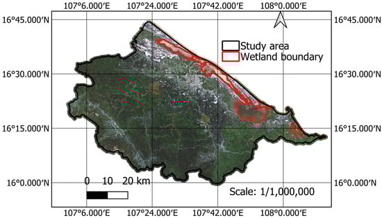
Figure 2.
The study area and wetland boundary (true color composite Sentinel-2 imagery). Data source: European Union/ESA/Copernicus.
The topography of Hue is characterized by diverse natural features that strongly influence its local climate and landscape structure. To the west lies the Truong Son Mountain range, with elevations ranging from low hills to peaks of approximately 1760 m [65]. The East Sea borders the area to the east. The Huong River flows through the urban core and divides the city into northern and southern sectors. The region also contains extensive coastal wetlands along the East Sea, most notably the Tam Giang–Cau Hai and Lap An lagoons. These wetlands cover a total area of approximately 257 km2 and function as key climate-regulating features. They provide substantial cooling during heat waves and help to moderate local thermal extremes.
Hue has a typical tropical monsoon rainforest climate, characterized by hot periods from March to August, when maximum temperatures can reach 35–40 °C. Annual rainfall is also high, averaging approximately 2500–3500 mm, with a pronounced rainy season from around October onward [65]. In recent years, due to the effects of climate change and urbanization, extreme heat has intensified, with peak temperatures often in the range of 37–40 °C. These heat waves amplified heat stress for residents in densely built-up areas [66]. Consequently, there is an urgent need to evaluate the cooling capacity of urban blue–green spaces and their influencing factors to support the mitigation of urban heat stress in Hue City.
2.2. Spatial Dataset Development
2.2.1. Remote Sensing Data
This study integrates multi-source remote sensing datasets to characterize land surface conditions across the study area (refer to Table 1). LST was derived from thermal observations acquired between 1 March and 31 July 2025. Elevation data were obtained from the NASA Shuttle Radar Topography Mission (SRTM) digital elevation model with a spatial resolution of 30 m; this data provides topographic context for the analysis. Data from Sentinel-2 imagery acquired between 1 January and 30 September 2025 was used to prepare a LULC map with four classes: bare land, built-up area, green space, and water body. This LULC map was subsequently used to derive the cooling-intensity map and urban morphological indicators for the study area. Moreover, road network information for Hue City was obtained from OpenStreetMap and extracted via the bbbike.org platform.

Table 1.
Remote sensing data.
2.2.2. Land Surface Temperature Retrieval
The analysis of wetland cooling intensity requires the retrieval of LST from Landsat-8 thermal data. In this study, LST data in Hue City was obtained from the USGS Landsat 8 Collection-2 Level-2 surface temperature product. The remote sensing data is retrieved from 1 March to 31 July 2025, a period characterized by multiple heatwaves in the region. A median operator is also applied to represent the typical thermal condition during the observation window while minimizing the influence of irregular data or outlier values.
It is noted that the thermal band ST_B10 is stored as a digital number that must be scaled to Kelvin. Hence, in the first step, the brightness temperature TB is computed as follows [67,68]:
where is the digital number of band 10 of the Landsat 8; 0.00341802 and 149.0 are two scaling factors.
Moreover, the emissivity-adjusted LST is computed as follows [69]:
where TS is the estimated LST measured in Celsius (°C); (10.8 µm) is the wavelength of emitted radiance; (1.438 10−2 mK), where h is Planck’s constant (6.626 10−34 Js), c denotes the velocity of light (2.997 108 m/s), and b is Boltzmann’s constant (1.38 10−23 J/K); 273.15 is the factor used for converting the temperature from Kelvin (K) to Celsius (°C); ε denotes a coefficient of the land surface emissivity, which is computed in the following manner [70]:
where is the vegetation proportion.
is computed by the Normalized Difference Vegetation Index (NDVI) as follows [67]:
where NDVImin and NDVImax denote the minimum and maximum values of NDVI, respectively.
Additionally, NDVI can be computed from Landsat 8’s bands in the following equation:
where SR_B5 and SR_B4 denote the near-infrared and red bands of Landsat 8, respectively.
Furthermore, a robust statistical procedure was applied to the LST data to characterize typical thermal conditions in the study area and reduce the influence of anomalous values as well as infrequent extremes. Specifically, the empirical distribution of all LST pixels over the study period was examined, and pixels with values below the 1st percentile or above the 99th percentile were treated as potential anomalies or outliers and excluded from subsequent analysis. Accordingly, only pixels with values in the range [20.23 °C, 42.35 °C] were retained. In other words, this procedure preserves the central 98% of the empirical LST distribution and discards the lowest 1% and highest 1% tails. Figure 3 presents the final LST in the study area from 1 March to 31 July 2025.
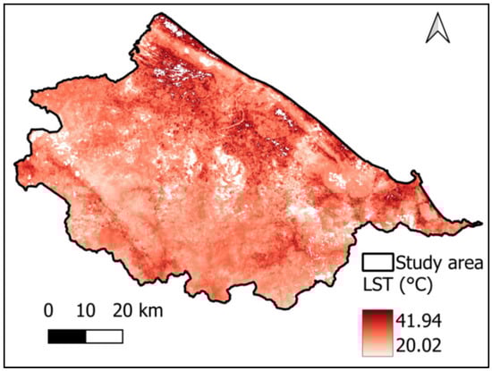
Figure 3.
Land surface temperature map.
2.2.3. The Spatial Dataset Used for Cooling Intensity Estimation
In the current work, cooling intensity is computed as the temperature difference between the mean LST of all built-up and bare-land pixels and the LST at a specific pixel surrounding a wetland. Accordingly, the cooling intensity at location [i, k] is calculated using the following expression:
where denotes mean LST of all built-up and bareland pixels; and are the cooling intensity and LST at location [i, k], respectively.
To derive the cooling intensity map, it is necessary to establish an LULC map for the study area. The LULC map was computed on the Google Earth Engine platform using a Random Forest classifier with 50 trees and Sentinel-2 multispectral bands. The classification output included four categories: bare land, built-up area, green space, and water body. For each class, 600 samples were collected; hence, the total number of data samples is 2400. The actual labels were interpreted and verified with the assistance of Google Earth Pro. The collected dataset was divided into a training set (80%) and a testing set (20%). The classification model attained high class-specific accuracies: 84.48% for bare land, 84.55% for built-up, 96.48% for green space, and 99.08% for water body. The LULC map (refer to Figure 4) was subsequently resampled to a spatial resolution of 30 m and prepared in QGIS 3.34.10.
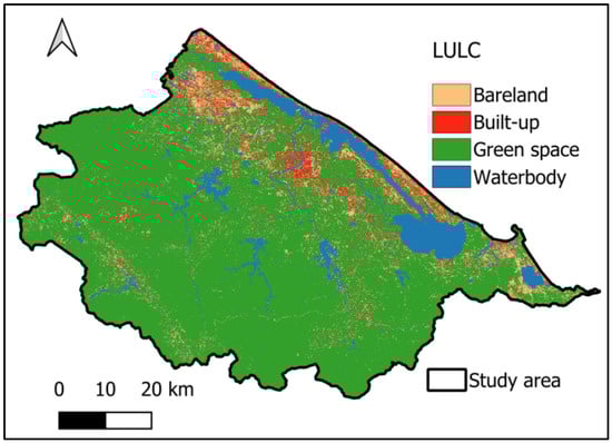
Figure 4.
LULC map.
Based on the established LULC and LST maps, a zonal operation can be used to compute the mean LST of all bare-land and built-up pixels. Let T (x) denote the LST at pixel x and let C (x) denote the LULC class at pixel x. The indicator set of all bare-land and built-up pixels can be defined as follows:
The mean LST over this zone is given by
where and are the average LST of all bare-land and built-up pixels and the total number of pixels in the .
This zonal mean serves as a reference temperature against which the cooling performance of the studied wetlands is evaluated. The cooling intensity at any pixel is therefore interpreted as how much cooler (positive values) or warmer (negative values) that pixel is relative to , that is, relative to the average thermal conditions of the combined bare-land and built-up surfaces. Based on the aforementioned zonal operation combining the LULC and LST maps, the mean LST of all bare-land and built-up pixels was found to be 34.09 °C. Accordingly, the cooling intensity map for the study area is illustrated in Figure 5.
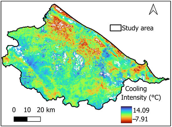
Figure 5.
Cooling intensity map.
Topographic characteristics are widely recognized as important factors influencing the spatial variability of LST, primarily through their regulation of air circulation and of solar radiation [71,72,73]. In this research, elevation (Figure 6a), slope (Figure 6b), and aspect (Figure 6c) are employed to characterize the influence of topography on the thermal behavior of riparian zones surrounding wetlands. Moreover, urban features are key determinants influencing LST and the resultant cooling intensity within urban environments [35,74]. Besides LULC, which describes the functional and compositional characteristics of the surface, this study also incorporates the densities of bare land, built-up areas, and green spaces to characterize urban morphology. These indicators are presented in Figure 7. It is noted that a morphological mean filter with a 210 m window size was applied to generate the density maps.
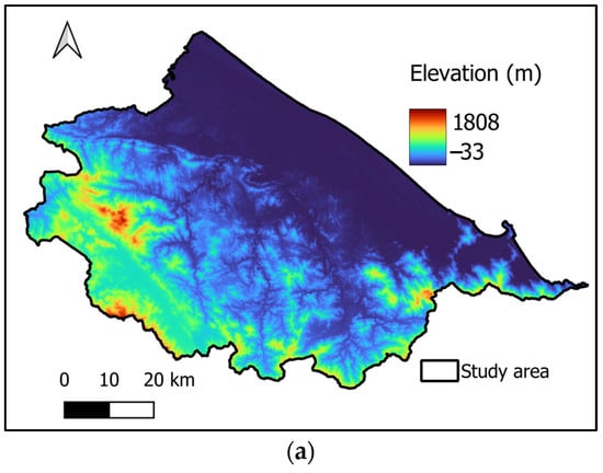
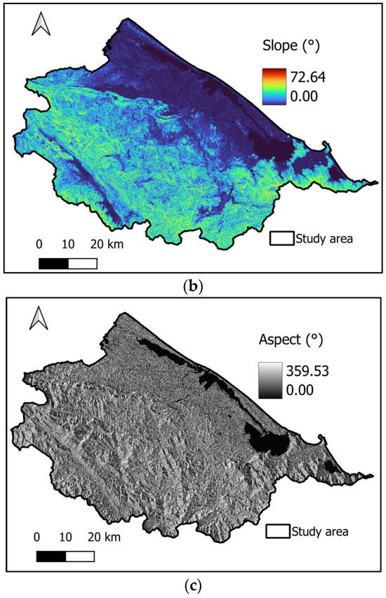
Figure 6.
Topographical features: (a) elevation, (b) slope, and (c) aspect.
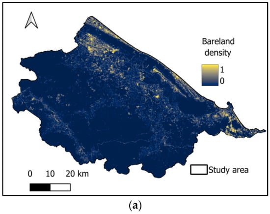
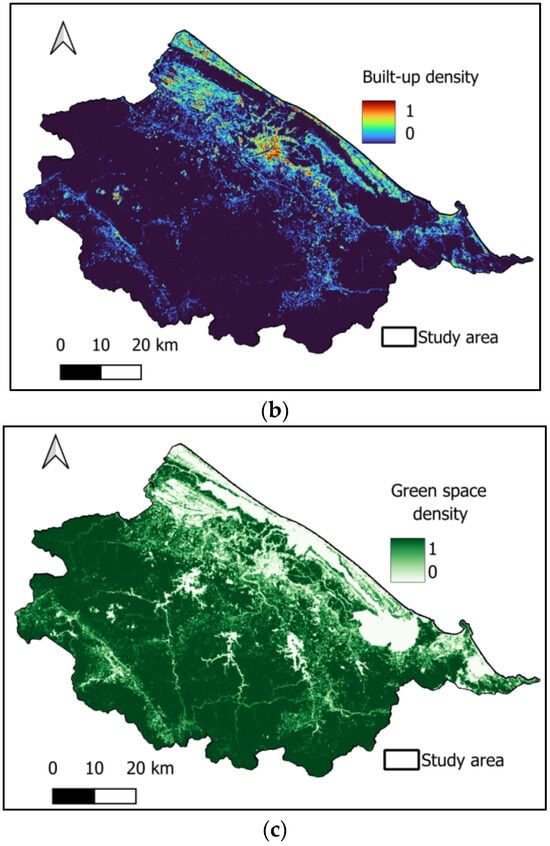
Figure 7.
Urban morphological features: (a) Bareland density, (b) built-up density, and (c) green space density.
Needless to say, urban morphological features play a significant role in shaping the spatial heterogeneity of LST as well as cooling intensity. High densities of built-up areas are typically associated with high LST due to the prevalence of impervious materials such as concrete and asphalt. These materials absorb and retain solar energy during the day. They release the heat slowly at night, thereby tending to intensify the UHI effect and diminish local cooling intensity. Similarly, bare land surfaces tend to exhibit higher LST because of limited vegetation cover. In contrast, green spaces—encompassing trees, shrubs, and grass-covered areas—act as effective thermal regulators through shading and evapotranspiration processes. Consequently, higher green space density tends to amplify cooling intensity, particularly around blue spaces.
The local urban context plays a vital role in determining the cooling intensity of wetlands, as surrounding landscape elements and anthropogenic structures jointly influence the spatial patterns of LST. Nearby lakes can provide additional sources of evaporative cooling, reinforcing the thermal moderation effect produced by wetlands. Similarly, proximity to coastlines often contributes to lower air and surface temperatures due to the sea–land breeze circulation and the high heat capacity of water bodies. Moreover, nearby rivers may also enhance the overall cooling performance of wetlands by expanding the area of moisture exchange and the cooling associated with evaporation from water surfaces. In contrast, infrastructures such as road networks tend to introduce considerable anthropogenic heat through vehicle emissions and thermal radiation from pavement materials. Therefore, this study incorporates proximity-based variables of distance to lake (Figure 8a), distance to coastline (Figure 8b), distance to river (Figure 8c), and distance to road (Figure 8d) to capture the combined effects of hydrographic influences, background cooling potential, and heat sources within the surrounding urban landscape. In addition to the aforementioned variables, distance to wetland boundary is used to characterize how the intensity of wetland-induced cooling varies with increasing separation from the wetland edge. This variable enables the analysis to capture the spatial variation in cooling benefits and to quantify the extent to which wetlands can effectively mitigate the heat stress in their surrounding areas.
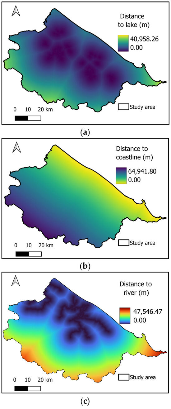
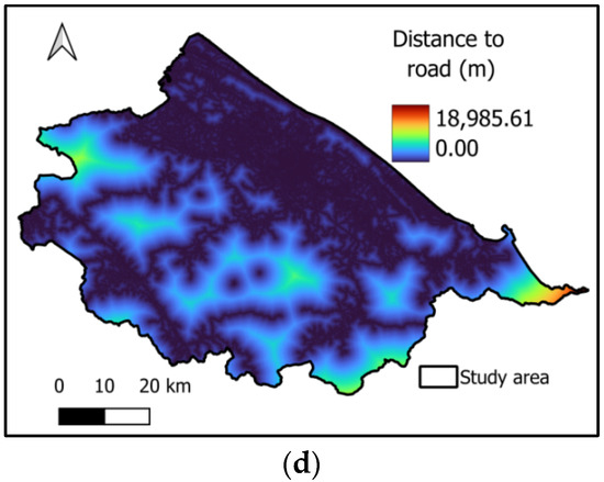
Figure 8.
Proximity-based features: (a) distance to lake, (b) distance to coastline, (c) distance to river, and (d) distance to road.
In this study, 100,000 sample points are randomly extracted within a 600 m buffer zone around the wetland boundary to represent the local thermal and environmental conditions. Accordingly, the dataset comprises 12 conditioning factors that characterize topography, land cover, urban morphology, and the context of the study area for predicting cooling intensity around the studied wetlands. The compiled spatial dataset is stored as a stack of raster layers, which includes the cooling intensity and all the explanatory variables. The statistical description of these conditioning factors is summarized in Table 2.
Table 2.
Statistical description of the variables in the dataset.
2.3. Light Gradient Boosting Machine Regressor for Cooling Intensity Estimation and Performance Evaluation Metrics
The Light Gradient Boosting Machine (LightGBM), proposed by Ke et al. [75], is an advanced gradient boosting framework that employs decision trees as its base learners. The LightGBM regressor used for cooling intensity estimation is illustrated in Figure 9. This machine learning approach is used to generalize a functional mapping between a set of explanatory variables and the cooling intensity. In general, LightGBM combines a set of weak regression trees to construct a more powerful predictive model. A LightGBM model is built in a stage-wise manner, where each successive iteration is designed to reduce the errors of the preceding model. The resulting ensemble model is obtained by integrating all decision trees into a single predictive function. In this study, the LightGBM model is implemented using the built-in functions provided in its official library (https://lightgbm.readthedocs.io/ (accessed on 12 November 2024)).
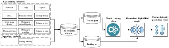
Figure 9.
The LightGBM model used for cooling intensity estimation.
The LightGBM regressor offers several major advantages for modeling large-scale, multivariate, and nonlinear spatial datasets. Its leaf-wise tree growth strategy, which repeatedly splits the leaf that maximally reduces the loss function, enables the model to discover complex, high-order interaction structures in the data [76]. This targeted splitting mechanism is particularly beneficial for geospatial applications, where relationships between environmental predictors and response variables often exhibit strong nonlinearity and spatial heterogeneity.
Moreover, the use of Gradient-based One-Side Sampling, which prioritizes samples with larger gradient magnitudes, substantially improves the training efficiency of LightGBM without compromising accuracy. Consequently, LightGBM can handle very large spatial datasets while maintaining feasible training times and memory usage. This capability is particularly important when working with multiple raster files and a large number of data points. LightGBM also incorporates Exclusive Feature Bundling (EFB), an efficient approach to dimensionality reduction that combines sparse, mutually exclusive features into bundles [77]. This technique minimizes redundancy in the feature space and reduces computational cost while retaining the most relevant predictors. For more details on the features of LightGBM, readers are referred to previous works [78,79].
LightGBM can help attain good predictive accuracy due to its efficiency in handling large datasets and complex nonlinear relationships. Nevertheless, as a tree-based ensemble approach, LightGBM operates as a black box. This fact brings about difficulties in interpreting the individual effect of an input feature. To address this issue, a partial dependence plot (PDP) [80] can be used to visualize how one selected predictor influences the model’s predicted cooling intensity while averaging the effects of all other variables. By illustrating the marginal relationships between a predictor and a target variable, a PDP provides valuable insights into the underlying behavior of the LightGBM model. In this study, the PDP analysis was conducted using the scikit-learn library [81]. We rely on a PDP to evaluate the effect of built-up density on the cooling performance of wetlands.
Within the framework of spatial modeling for cooling intensity, we aim to accurately predict the spatial variation in cooling intensity from a set of explanatory factors. Assessing model performance is crucial for determining how well the machine learning approach captures the underlying spatial relationships. Accordingly, this study relies on the Root Mean Square Error (RMSE), Mean Absolute Error (MAE), and the coefficient of determination (R2). These metrics are calculated as follows:
where ti and yi are the actual and estimated cooling intensity values of the ith data point, respectively. N denotes the total number of data points.
The performance of a LightGBM–based regression model for predicting cooling intensity can be effectively assessed using the aforementioned metrics. RMSE measures the average magnitude of prediction errors; it assigns greater weight to larger deviations and thus is sensitive to outliers. MAE reflects the average absolute difference between predicted and observed values; this index offers a more interpretable measure of typical prediction accuracy. Meanwhile, the coefficient of determination indicates how well the model explains the variance in the observed data, with higher values signifying stronger predictive relationships. R2 can be used to assess the overall explanatory power and generalization capability of the LightGBM model in predicting spatial cooling intensity patterns.
3. Machine Learning-Based Simulation Framework for Estimating the Effective Cooling Range of Wetlands
Urban planners need to estimate how far the cooling effect of wetlands extends into surrounding areas to support zoning decisions, building regulations, and climate-adaptation strategies. This estimate also provides insight into the cooling capacity and spatial influence of wetlands. Based on the analysis result, it is able to identify which conditions deliver the strongest local temperature mitigation and where additional preservation or restoration would be most prioritized. Moreover, characterizing the effective cooling range enables comparisons of wetland configurations and landscape settings. In the present work, a model-based simulation framework, which is essentially a sensitivity analysis approach, is used to explore how predicted cooling intensity responds to distance from wetlands under varying background conditions and to derive an effective cooling range.
The employed simulation framework offers several benefits. It is fully data-driven and relies on an empirically trained LightGBM model to infer cooling–distance relationships directly from observations. Once the model is trained, the simulation procedure is entirely automated. It systematically generates cooling profiles and detects the effective cooling range without the need for manual data processing. This process can be easily extended to larger datasets or additional wetlands.
The simulation framework (Figure 10) relies on a Monte Carlo–style procedure that uses the trained LightGBM regressor to perform a sensitivity analysis of predicted cooling intensity with respect to distance from the wetland and to estimate the effective cooling distance. This distance is defined as the first considerable local minimum in the predicted cooling-intensity profile along a distance gradient from the wetland. The model is first fitted to predict cooling intensity from a set of explanatory variables. A random observation from the original dataset is then selected. The model is used to generate synthetic cooling profiles by systematically varying only the distance to the wetland while holding all other features fixed. A regular distance grid from 0 to 600 m in 30 m steps is used to approximate the spatial cooling profile away from the wetland boundary. The step size of 30 m is selected to match the spatial resolution of the Landsat imagery.
Figure 10.
Workflow of the model-based simulation and sensitivity analysis used to estimate the wetland cooling range.
This process yields one cooling curve per simulation. For each predicted cooling curve, a moving average with a smoothing window of 3 is applied to reduce small, noisy fluctuations so that only meaningful changes in cooling intensity can be recognized. This window length was chosen to smooth minor point-to-point variations while preserving the overall shape of the cooling profile. After a specified number of simulations (N), all the cooling curves are then subsequently combined to compute a mean cooling profile. The framework then analyzes the mean cooling profile to locate the first local minimum. To eliminate minor fluctuations in the profile, a local minimum is considered valid only if it represents a drop of at least 0.1 °C from the highest smoothed value observed so far. This threshold is chosen to distinguish meaningful local minima from negligible variation. The corresponding distance on the grid is interpreted as the effective cooling range. In other words, this is the distance beyond which the marginal cooling effect of the wetland becomes substantially weaker. Although the chosen framework parameters (30 m distance step, smoothing window of 3, and 0.1 °C drop threshold) are reasonable for the present study, the estimated effective cooling distance may vary to some extent if different parameter values are adopted.
4. Prediction Results
This section presents the results of cooling intensity estimation using the employed LightGBM regressor. The machine learning approach was constructed and tested with a spatial dataset collected in the coastal area of Hue City. Notably, a 600 m buffer surrounding wetlands was defined, within which 100,000 random sampling points were generated. To model the spatial variation in the cooling intensity, 12 explanatory variables were used. The dataset was randomly divided into two subsets: 70% for training and 30% for testing. It should be noted that, because the samples are spatially continuous, this random split may affect the model’s performance due to spatial autocorrelation among nearby observations. The LightGBM model utilized the training data to infer a nonlinear relationship between those 12 conditioning factors and the wetlands’ cooling intensity.
In this study, the hyperparameters of the LightGBM regressor were tuned using 5-fold cross-validation on the training dataset to achieve a balance between model accuracy and generalization. The training set was randomly partitioned into five mutually exclusive folds; for each candidate hyperparameter configuration, the model was fitted on four folds and evaluated on the remaining fold. This process was repeated so that each fold served once as validation. The average RMSE across the five folds was used to assess each configuration, and the hyperparameters with the lowest mean RMSE were selected. The hyperparameters include the maximum depth of each decision tree (MTD), the learning rate (γ), the number of boosting iterations (NBI), the L2 regularization coefficient (λR), and the L1 regularization coefficient (αR). The selected model’s configuration is as follows: MTD = 9, γ = 0.2, NBI = 800, λR = 0.01, and αR = 0.001.
It is noted that the maximum depth of each decision tree dictates the complexity of each decision tree, where deeper trees can better capture intricate variations in cooling intensity but may also increase the risk of overfitting. The learning rate defines the step size by which the model updates in each boosting iteration; it influences both convergence speed and model stability. The number of boosting iterations determines the total number of trees in the ensemble, where a larger number often enhances predictive performance at the cost of longer training time and potential overfitting. Additionally, the two regularization coefficients were utilized to control model complexity and prevent overfitting by penalizing large coefficients.
The model’s performance is summarized in Figure 11. As can be seen from the experimental results, the LightGBM regressor demonstrates strong predictive performance in both training and testing phases, with only a moderate reduction in accuracy when applied to unseen data. In the training phase, the model attains RMSE = 0.80, MAE = 0.56, and R2 = 0.96; this fact indicates that it explains about 96% of the variance in the training data. In the testing phase, the model maintains strong predictive performance, with RMSE = 1.15, MAE = 0.77, and R2 = 0.91; the outcome implies that roughly 91% of the variance in cooling intensity is captured by the model when predicting novel samples. The ratio of testing to training RMSE (1.44) shows an increase in error, which suggests a certain degree of overfitting. This fact is understandable since the problem at hand involves a large-scale dataset of 100,000 samples with 12 predictors derived from multiple data sources. In general, the results in terms of R2 (>90%) indicate that the model retains good generalization given the complexity of the task. These levels of accuracy can be regarded as satisfactory for the current task of modeling wetland cooling intensity.
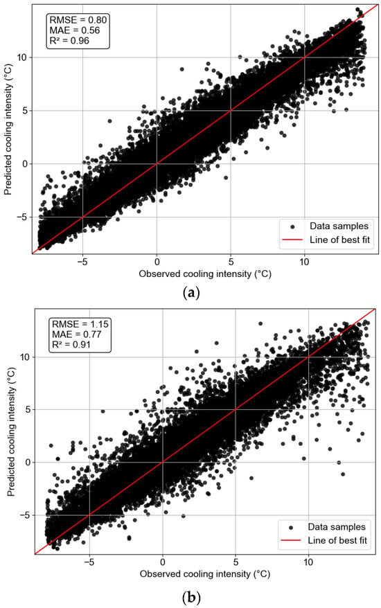
Figure 11.
LightGBM: (a) Training phase and (b) Testing phase.
Figure 12 illustrates the residual distributions for both the training and testing stages, which appear approximately symmetric and centered around zero. This fact indicates that there is no systematic bias in the estimation of cooling intensity. In the training phase, residuals are sharply concentrated, with a mean close to 0 °C and a relatively small standard deviation (0.8), whereas in the testing phase, the mean error remains near zero but the spread of residuals slightly increases (1.15), as reflected by a larger standard deviation. These patterns indicate that the LightGBM model produces small, well-controlled residuals in both phases.
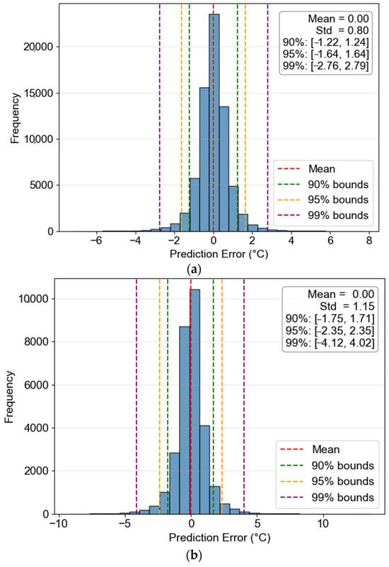
Figure 12.
Error histogram: (a) Training phase and (b) testing phase.
To further quantify the discrepancy between the observed cooling intensity and the LightGBM prediction, this study relies on the regression error characteristic curve (REC) [82]. In general, REC shows the absolute deviation on the x-axis against the proportion of samples with errors below each deviation level on the y-axis. As illustrated in Figure 13, the RECs summarize the proportion of predictions that fall within specified error bounds for both the training and testing phases. In the training phase, roughly 90% and 95% of samples exhibit absolute errors smaller than about 1.25 °C and 1.67 °C, respectively. Meanwhile, in the testing phase, the corresponding thresholds are approximately 1.77 °C and 2.38 °C. The curves are relatively steep and located toward the upper-left region of the plots. This characteristic indicates that a high proportion of predictions is associated with small deviations in both phases and confirms the reliability of the machine learning model for cooling intensity estimation.
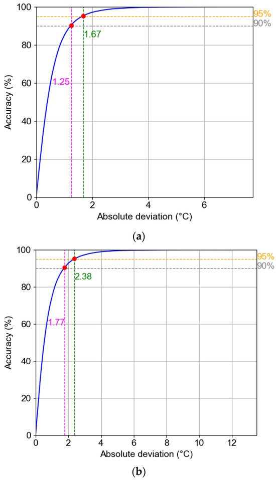
Figure 13.
RECs: (a) Training phase and (b) testing phase.
The LightGBM model can also be used to derive importance scores of the features by aggregating how often each feature is used to split nodes across all regression trees in the ensemble. Thus, higher scores indicate crucial predictors that more frequently and substantially reduce the prediction error. Figure 14 shows that hydrological proximity considerably influences cooling intensity in the region. The proximity to rivers, coastlines, and nearby lakes emerges as the most influential set of predictors, followed by distance to wetland boundaries, distance to roads, and green space density. Meanwhile, topographic variables (elevation, slope, aspect) and built-up or bare-land density have moderate contributions. Moreover, LULC plays a minor role in explaining cooling intensity.
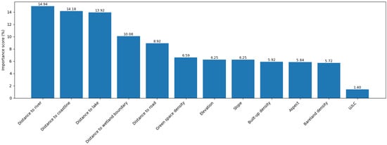
Figure 14.
Feature importance scores yielded by LightGBM.
Figure 15 summarizes the result of the machine learning-based simulation framework used to quantify how the mean cooling intensity varies with distance from the wetland boundary. In this framework, the trained LightGBM regressor predicts cooling intensity along a regular distance grid extending from 0 to 600 m from the wetland boundary; the data was sampled at 30 m intervals. The convergence diagnostics for the simulation framework is summarized in Table 3. Across different simulation iterations, numerical convergence was assessed from the point-wise average difference (εMean) and maximum absolute difference (εMax) between successive profiles. The tolerance thresholds εMean and εMax are set to be 0.01 °C and 0.05 °C, respectively.
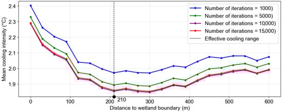
Figure 15.
Mean cooling intensity vs. distance to wetland boundary.
Table 3.
Convergence diagnostics for the simulation framework.
As indicated by the results, the change between 10,000 and 15,000 iterations (average 0.006 °C; maximum 0.008 °C) satisfies both convergence criteria. Consequently, 10,000 iterations were adopted for inferring the cooling performance. As shown in Figure 15, the first marked local minimum of the mean cooling-intensity profile occurs at 210 m from the wetland boundary, which is interpreted as the effective cooling range. Within this interval, the mean cooling intensity is approximately 2.02 °C.
Moreover, built-up density is a crucial parameter for zoning regulation in the study area. This study relies on a PDP analysis to inspect the effect of built-up density on the wetland cooling-intensity predictions in riparian zones. The outcome is reported in Figure 16. As can be seen in this figure, built-up density exerts a strong, approximately monotonic negative effect on the wetland cooling intensity. This fact implies that sparsely developed areas near wetlands are associated with substantial cooling. As built-up density increases, cooling intensity declines sharply. The cooling effect becomes neutral at a density value of roughly 0.45. Beyond this value, higher built-up density leads to further heat stress. It is noted that this threshold should be interpreted as a model-based reference specific to the current dataset.
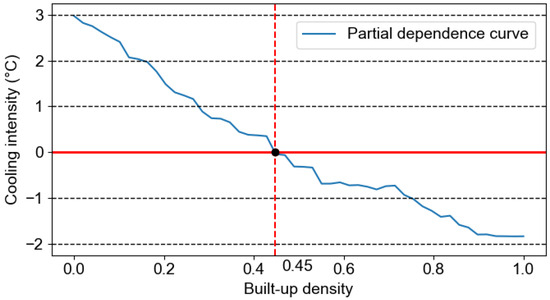
Figure 16.
Effect of built-up density on cooling intensity.
5. Discussion
As shown by the experimental results, LightGBM achieves strong performance in estimating wetland cooling intensity. This outcome reflects the fact that the model possesses notable advantages that are well aligned with the task at hand. As a gradient-boosting framework, LightGBM is well-suited to capture the nonlinear interactions and spatial heterogeneity inherent in multivariate GIS and remote-sensing data describing wetlands and their surroundings. The incorporation of regularization parameters enables the model to remain sufficiently flexible to learn complex patterns while controlling overfitting, as evidenced by the high coefficients of determination (R2 = 0.96 for training and 0.91 for testing) and the relatively low RMSE and MAE values in both phases.
The employed metric indicates that the model explains more than 90% of the variance in cooling intensity, which is highly desirable given the large sample size of 100,000 data points and the multiple predictors involved. The success of LightGBM in this study is also consistent with previous work reporting high accuracy for LST estimation [83,84] and large-scale remote sensing applications [76,85]. Hence, the present findings further support the suitability of LightGBM as a robust tool for modeling the cooling effects of wetlands in complex geospatial settings.
Additionally, the feature importance analysis indicates that hydrological proximity exerts a dominant control on wetland cooling intensity. The distances to the river, coastline, and lake constitute the most influential group of predictors. This outcome reflects the role of surface water bodies in defining the local hydrographic context and connectivity around each wetland. These hydrological features act synergistically to govern cooling performance in the coastal study region, where rivers and lakes form a complex network of urban blue spaces.
Distance to the wetland boundary also ranks among the most important factors; this fact implies the central role of wetlands in regulating local thermal conditions. Moreover, the impact of built-up area is evident and aligns with earlier work showing a negative relationship between the cooling capacity of urban wetlands and the density of surrounding buildings [58]. By contrast, LULC has only a minor contribution because key aspects of urban form and neighborhood morphology are already captured by built-up, bare-land, and green space densities; this observation agrees with prior results indicating that local land cover classes can be less influential than broader patterns of urbanization and greenness in explaining spatial variations in surface thermal behavior [44].
The machine learning-based simulation indicates that wetlands in the study area exert a considerable local cooling effect, with an effective cooling range of 210 m and a mean cooling intensity of about 2.0 °C within this zone. This distance exceeds the maximum cooling range of 157 m reported by Liu et al. [28], who also employed a 600 m buffer-zone analysis. The magnitude of cooling estimated in the current study is also comparable to that of Gao et al. [31], who show that wetlands can achieve temperature reductions of −1.20 ± 0.77 K. Similarly, Xie et al. [86] also reported a cooling effect of 2.61 °C for small, connected wetlands. These results support the view that the effective cooling range and mean cooling intensity of wetlands are highly context dependent; they vary with local climatic, geographical, and landscape conditions.
Overall, the results of this study highlight wetlands as crucial cooling elements that require protection and careful planning in their riparian zones. The partial dependence analysis shows that built-up density has a negative effect on wetland cooling intensity. In light of this, our results suggest that building regulations in the vicinity of wetlands may consider keeping built-up density below a data-driven reference level of roughly 45%. In addition, green spaces in riparian zones should be encouraged since vegetation is known to mitigate urban heat and enhance the performance of adjacent blue spaces [62].
Urban expansion and land-use conversion are placing substantial pressure on wetland preservation worldwide [25,87]. Nevertheless, because water surfaces often provide stronger cooling than vegetation alone [88], local authorities should prioritize the conservation and hydrological integrity of wetland systems to sustain their function as effective nature-based solutions for local heat mitigation. This priority is justified by evidence that hydrological disconnection and spatial fragmentation can negatively affect the cooling capacity of wetlands [86].
6. Limitations and Future Perspectives
This study has several limitations that should be acknowledged. First, local meteorological conditions in Hue City—such as wind speed, humidity, and precipitation—were not incorporated, which may limit the ability to fully separate the influence of atmospheric factors from that of land-surface characteristics on cooling intensity. Second, the current analysis did not distinguish between different types of green space around wetlands (e.g., parks, agricultural land, etc.). Accordingly, the potential differences in cooling performance associated with specific vegetation types could not be accurately assessed. Third, although LightGBM performs well, more advanced machine learning approaches—such as deep learning or other ensemble frameworks—could be explored in future works to further reveal the drivers of urban wetland cooling. Finally, the LST data were derived from Landsat-8 at a spatial resolution of 30 m, which constrains the ability to capture fine-scale thermal heterogeneity and micro-cooling effects.
Accordingly, future works could integrate local meteorological observations to examine the roles of atmospheric conditions and land-surface characteristics in shaping wetland cooling intensity. The analysis could also be enhanced by differentiating among specific types of green space around wetlands to better quantify how vegetation structure influences cooling performance. Furthermore, more detailed wetland mapping that distinguishes different wetland types and evaluates their cooling effects separately should be considered, using higher-resolution or complementary data sources such as detailed wetland inventories, Synthetic Aperture Radar (SAR) imagery, or field surveys.
It would be valuable to compare LightGBM with other advanced data-driven approaches to identify capable tools for geospatial modeling of cooling intensity and landscape optimization, particularly in the tasks of landscape optimization and design of blue–green spaces. Using higher-resolution thermal data would also allow investigation of fine-scale cooling patterns within narrow riparian zones and small wetland fragments in Hue’s urban core. Finally, incorporating data from multiple cities with different climatic conditions and urban forms would significantly enhance the generalizability and practical applicability of the proposed framework.
7. Conclusions
The research framework integrated remote sensing, geospatial analysis, and machine learning to quantify both the cooling intensity and the effective cooling range of wetlands in the coastal region of Hue City, Vietnam. Remote sensing data were used to establish a set of influencing factors, including distance to wetland boundary, urban morphology, topography, LULC, and proximity-based features. Accordingly, 12 conditioning factors were employed to capture the spatial variation in cooling intensity in the surrounding region of wetlands. To construct a spatial dataset, 100,000 sample points were randomly generated within a 600 m buffer around the wetland boundary.
A LightGBM regressor was employed to generalize the relationship between the conditioning factors and the cooling intensity. The model demonstrated strong predictive performance and explained approximately 91% of the variance in cooling intensity on the testing dataset. This fact indicates that LightGBM can effectively handle the large sample size and complex nonlinear interactions present in the data. The trained model was then used to construct a simulation framework that estimates the effective cooling range. The framework is fully data-driven and can be readily extended to analyze other wetlands. The simulation results show that the effective cooling range of the studied wetlands is 210 m. Within this zone, the mean cooling intensity is approximately 2.02 °C; this result confirms that wetlands act as strong local cooling sources in the urban and peri-urban landscape of Hue City.
To further interpret model behavior and support urban planning in the study area, a partial dependence analysis was conducted for built-up density. The PDP illustrates how changes in built-up density around wetlands influence predicted cooling intensity while averaging over other variables. The analysis reveals a clear decline in cooling intensity as built-up density increases. Importantly, the result obtained from PDP indicates that built-up density in the riparian zones of wetlands should not exceed 45%. However, this threshold should be interpreted as a model-based planning reference for Hue City rather than as a universal hard limit.
Recent years have seen intensifying extreme heat in the urban center of Hue City due to the combined effects of climate change and rapid urbanization. This fact accentuates the importance of wetlands as crucial nature-based assets for mitigating urban heat. Land-use planners and decision-makers, therefore, need a clear understanding of the cooling effects of wetlands. The findings of this study provide a more detailed picture of the cooling performance of wetlands in Hue City and clarify how their cooling capacity varies with distance and surrounding urban form. These results can inform planning strategies that aim to deploy wetlands and associated blue–green infrastructure as nature-based solutions for enhancing urban thermal comfort.
Funding
This research received no external funding.
Data Availability Statement
The original data presented in the study are openly available in GitHub at https://github.com/NhatDucHoang/WetlandCoolingIntensity_HueCity (accessed on 11 January 2026).
Conflicts of Interest
The author declares no conflicts of interest.
Abbreviations
The following abbreviations are used in this manuscript:
| LST | Land Surface Temperature |
| LULC | Land Use or Land Cover |
| UHI | Urban Heat Island |
| GEE | Google Earth Engine |
| LightGBM | Light Gradient Boosting Machine |
| GIS | Geographic Information System |
| SRTM | Shuttle Radar Topography Mission |
| NDVI | Normalized Difference Vegetation Index |
| EFB | Exclusive Feature Bundling |
| PDP | Partial Dependence Plot |
| RMSE | Root Mean Square Error |
| MAE | Mean Absolute Error |
| REC | Regression Error Characteristic Curve |
References
- Estoque, R.C.; Murayama, Y.; Myint, S.W. Effects of landscape composition and pattern on land surface temperature: An urban heat island study in the megacities of Southeast Asia. Sci. Total Environ. 2017, 577, 349–359. [Google Scholar] [CrossRef]
- Santhanam, H.; Majumdar, R. Quantification of green-blue ratios, impervious surface area and pace of urbanisation for sustainable management of urban lake—Land zones in India -a case study from Bengaluru city. J. Urban Manag. 2022, 11, 310–320. [Google Scholar] [CrossRef]
- Vu, A.T.; Ngo, D.A.; Nguyen, T.P.H.; Nguyen, C.G. Applying object-based approach to monitor urban expansion in Ha Long city, Vietnam, during 2000-2023 from multi-date Landsat satellite imagery. Eur. J. Remote Sens. 2024, 57, 2398108. [Google Scholar] [CrossRef]
- Do, A.N.T.; Tran, H.D.; Do, T.A.T. Impacts of urbanization on heat in Ho Chi Minh, southern Vietnam using U-Net model and remote sensing. Int. J. Environ. Sci. Technol. 2024, 21, 3005–3020. [Google Scholar] [CrossRef]
- Ampatzidis, P.; Kershaw, T. A review of the impact of blue space on the urban microclimate. Sci. Total Environ. 2020, 730, 139068. [Google Scholar] [CrossRef]
- Perkins-Kirkpatrick, S.E.; Lewis, S.C. Increasing trends in regional heatwaves. Nat. Commun. 2020, 11, 3357. [Google Scholar] [CrossRef]
- Jones, L.; Fletcher, D.; Fitch, A.; Kuyer, J.; Dickie, I. Economic value of the hot-day cooling provided by urban green and blue space. Urban For. Urban Green. 2024, 93, 128212. [Google Scholar] [CrossRef]
- Kim, S.W.; Brown, R.D. Urban heat island (UHI) intensity and magnitude estimations: A systematic literature review. Sci. Total Environ. 2021, 779, 146389. [Google Scholar] [CrossRef]
- Yadav, N.; Rajendra, K.; Awasthi, A.; Singh, C.; Bhushan, B. Systematic exploration of heat wave impact on mortality and urban heat island: A review from 2000 to 2022. Urban Clim. 2023, 51, 101622. [Google Scholar] [CrossRef]
- Ganeshan, M.; Murtugudde, R.; Imhoff, M.L. A multi-city analysis of the UHI-influence on warm season rainfall. Urban Clim. 2013, 6, 1–23. [Google Scholar] [CrossRef]
- Piracha, A.; Chaudhary, M.T. Urban Air Pollution, Urban Heat Island and Human Health: A Review of the Literature. Sustainability 2022, 14, 9234. [Google Scholar] [CrossRef]
- Manoli, G.; Fatichi, S.; Schläpfer, M.; Yu, K.; Crowther, T.W.; Meili, N.; Burlando, P.; Katul, G.G.; Bou-Zeid, E. Magnitude of urban heat islands largely explained by climate and population. Nature 2019, 573, 55–60. [Google Scholar] [CrossRef] [PubMed]
- Wong, L.P.; Alias, H.; Aghamohammadi, N.; Aghazadeh, S.; Nik Sulaiman, N.M. Urban heat island experience, control measures and health impact: A survey among working community in the city of Kuala Lumpur. Sustain. Cities Soc. 2017, 35, 660–668. [Google Scholar] [CrossRef]
- Le Phuc, C.L.; Nguyen, H.S.; Dao Dinh, C.; Tran, N.B.; Pham, Q.B.; Nguyen, X.C. Cooling island effect of urban lakes in hot waves under foehn and climate change. Theor. Appl. Climatol. 2022, 149, 817–830. [Google Scholar] [CrossRef]
- Pham Thi, L.; Pham Thanh, H.; Phan Van, T.; Vu Thuan, Y. Variability of heatwaves across Vietnam in recent decades. Vietna. J. Earth Sci. 2023, 45, 517–530. [Google Scholar] [CrossRef]
- Hoang, T.L.T.; Dao, H.N.; Cu, P.T.; Tran, V.T.T.; Tong, T.P.; Hoang, S.T.; Vuong, V.V.; Nguyen, T.N. Assessing heat index changes in the context of climate change: A case study of Hanoi (Vietnam). Front. Earth Sci. 2022, 10, 897601. [Google Scholar] [CrossRef]
- Kien, N.D.; My, N.H.D.; Thu, D.T.A.; Tri, T.T.C.; Son, N.H.; Phong, T.K.; Tin, H.C.; Lan, N.H.; Thang, T.B.; The, B.D.; et al. Valuation of a Heatwave Early Warning System for Mitigating Risks Associated with Heat-Related Illness in Central Vietnam. Sustainability 2023, 15, 15342. [Google Scholar] [CrossRef]
- Kumar, P.; Debele, S.E.; Khalili, S.; Halios, C.H.; Sahani, J.; Aghamohammadi, N.; Andrade, M.d.F.; Athanassiadou, M.; Bhui, K.; Calvillo, N.; et al. Urban heat mitigation by green and blue infrastructure: Drivers, effectiveness, and future needs. Innovation 2024, 5, 100588. [Google Scholar] [CrossRef]
- Thien, B.B.; Phuong, V.T.; Alexsander, I.R.; Denis, K.O. Machine learning-based assessment of land use change effects on land surface temperature fluctuations in Ho Chi Minh city, Vietnam. Environ. Monit. Assess. 2025, 197, 1097. [Google Scholar] [CrossRef]
- Theeuwes, N.E.; Solcerová, A.; Steeneveld, G.J. Modeling the influence of open water surfaces on the summertime temperature and thermal comfort in the city. J. Geophys. Res. Atmos. 2013, 118, 8881–8896. [Google Scholar] [CrossRef]
- Giang, N.B.; Huong, D.T.V. The Cooling Effects of Water Body System on Land Surface Temperature in Vicinity Regions: A Case Study in Hue City, Vietnam. In International Conference on Global Changes and Sustainable Development in Asian Emerging Market Economies: Volume 2; Springer Nature: Cham, Switzerland, 2024; pp. 645–664. [Google Scholar]
- Gunawardena, K.R.; Wells, M.J.; Kershaw, T. Utilising green and bluespace to mitigate urban heat island intensity. Sci. Total Environ. 2017, 584–585, 1040–1055. [Google Scholar] [CrossRef] [PubMed]
- Pan, Z.; Xie, Z.; Wu, L.; Pan, Y.; Ding, N.; Liang, Q.; Qin, F. Simulation of Cooling Island Effect in Blue-Green Space Based on Multi-Scale Coupling Model. Remote Sens. 2023, 15, 2093. [Google Scholar] [CrossRef]
- Zhang, Z.; Chen, F.; Barlage, M.; Bortolotti, L.E.; Famiglietti, J.; Li, Z.; Ma, X.; Li, Y. Cooling Effects Revealed by Modeling of Wetlands and Land-Atmosphere Interactions. Water Resour. Res. 2022, 58, e2021WR030573. [Google Scholar] [CrossRef]
- Sousa, C.A.M.; Cunha, M.E.; Ribeiro, L. Tracking 130 years of coastal wetland reclamation in Ria Formosa, Portugal: Opportunities for conservation and aquaculture. Land Use Policy 2020, 94, 104544. [Google Scholar] [CrossRef]
- Meng, Z.; Shen, G.; Liao, J.; Guo, Y.; Li, J. Urban wetland landscape patterns and cooling effects in Guilin utilizing GF-1/6 and SDGSAT-1 data. Int. J. Digit. Earth 2025, 18, 2467985. [Google Scholar] [CrossRef]
- Brazel, A.; Ruiz-Aviles, V.; Hagen, B.; Davis, J.M.; Pijawka, D. Cooling Effects and Human Comfort of Constructed Wetlands in Desert Cities: A Case Study of Avondale, Arizona. Sustainability 2024, 16, 5456. [Google Scholar] [CrossRef]
- Liu, L.; He, H.; Cai, Y.; Hang, J.; Liu, J.; Liu, L.; Jiang, P.; He, H. Cooling effects of wetland parks in hot and humid areas based on remote sensing images and local climate zone scheme. Build. Environ. 2023, 243, 110660. [Google Scholar] [CrossRef]
- Chen, J.; Wen, J.; Kang, S.; Meng, X.; Tian, H.; Ma, X.; Yuan, Y. Assessments of the factors controlling latent heat flux and the coupling degree between an alpine wetland and the atmosphere on the Qinghai-Tibetan Plateau in summer. Atmos. Res. 2020, 240, 104937. [Google Scholar] [CrossRef]
- Shahjahan, A.T.M.; Ahmed, K.S.; Said, I.B. Study on Riparian Shading Envelope for Wetlands to Create Desirable Urban Bioclimates. Atmosphere 2020, 11, 1348. [Google Scholar] [CrossRef]
- Gao, X.; Yan, Z.; Bao, L.; Li, X.; Gao, L.; Yu, L. Satellite observation reveals wetland-induced local cooling moderated by regional climate gradients. Sci. Remote Sens. 2025, 12, 100292. [Google Scholar] [CrossRef]
- Diem, P.K.; Nguyen, C.T.; Diem, N.K.; Diep, N.T.H.; Thao, P.T.B.; Hong, T.G.; Phan, T.N. Remote sensing for urban heat island research: Progress, current issues, and perspectives. Remote Sens. Appl. Soc. Environ. 2024, 33, 101081. [Google Scholar] [CrossRef]
- Ullah, S.; Khan, M.; Qiao, X. Evaluating the impact of urbanization patterns on LST and UHI effect in Afghanistan’s Cities: A machine learning approach for sustainable urban planning. In Environment, Development and Sustainability; Springer Nature: Cham, Switzerland, 2025. [Google Scholar] [CrossRef]
- Bera, B.; Shit, P.K.; Saha, S.; Bhattacharjee, S. Exploratory analysis of cooling effect of urban wetlands on Kolkata metropolitan city region, eastern India. Curr. Res. Environ. Sustain. 2021, 3, 100066. [Google Scholar] [CrossRef]
- Tran, V.-D.; Hoang, N.-D. Machine Learning Insight into the Cooling Intensity of Urban Blue-Green Spaces During Heatwaves. Sustainability 2025, 17, 9824. [Google Scholar] [CrossRef]
- Hosen, M.I.; Hasan, M.M.; Talha, M.; Akter, M.M.; Nasher, N.M.R. Exploring the cooling benefits of Urban Lakes: A multi-year analysis of Dhaka, Bangladesh. HydroResearch 2025, 8, 361–373. [Google Scholar] [CrossRef]
- Islam, M.R.; Shahfahad; Talukdar, S.; Rihan, M.; Rahman, A. Evaluating cooling effect of blue-green infrastructure on urban thermal environment in a metropolitan city: Using geospatial and machine learning techniques. Sustain. Cities Soc. 2024, 113, 105666. [Google Scholar] [CrossRef]
- Khalil, M.; Kumar, J.S. Assessing Urban Heat Island Intensity in Damascus City Using Google Earth Engine and Landsat 8 and 9: A Comparative Analysis. Remote Sens. Earth Syst. Sci. 2025, 8, 576–592. [Google Scholar] [CrossRef]
- Li, F.; Yigitcanlar, T.; Nepal, M.; Nguyen, K.; Dur, F. Machine learning and remote sensing integration for leveraging urban sustainability: A review and framework. Sustain. Cities Soc. 2023, 96, 104653. [Google Scholar] [CrossRef]
- Snaiki, R.; Merabtine, A. Recent advances on machine learning techniques for urban heat island applications: A review and new horizons. Sustain. Cities Soc. 2025, 134, 106943. [Google Scholar] [CrossRef]
- Mansourmoghaddam, M.; Rousta, I.; Ghafarian Malamiri, H.; Sadeghnejad, M.; Krzyszczak, J.; Ferreira, C.S.S. Modeling and Estimating the Land Surface Temperature (LST) Using Remote Sensing and Machine Learning (Case Study: Yazd, Iran). Remote Sens. 2024, 16, 454. [Google Scholar] [CrossRef]
- Zhang, Y.; Ge, J.; Wang, S.; Dong, C. Optimizing urban green space configurations for enhanced heat island mitigation: A geographically weighted machine learning approach. Sustain. Cities Soc. 2025, 119, 106087. [Google Scholar] [CrossRef]
- Toscan, P.C.; Seong, K.; Jiao, J.; Ribeiro, C.A.L.R.; Carvalho, F.A.C.; Oliveira, M.L.S.; Pereira, E.B. Impact of nature-based solutions (NBS) on urban surface temperatures and land cover changes using remote sensing and machine learning. Remote Sens. Appl. Soc. Environ. 2025, 39, 101721. [Google Scholar] [CrossRef]
- Hoang, N.-D.; Nguyen, Q.-L. Geospatial Analysis and Machine Learning Framework for Urban Heat Island Intensity Prediction: Natural Gradient Boosting and Deep Neural Network Regressors with Multisource Remote Sensing Data. Sustainability 2025, 17, 4287. [Google Scholar] [CrossRef]
- Budzik, G.; Sylla, M.; Kowalczyk, T. Understanding Urban Cooling of Blue–Green Infrastructure: A Review of Spatial Data and Sustainable Planning Optimization Methods for Mitigating Urban Heat Islands. Sustainability 2025, 17, 142. [Google Scholar] [CrossRef]
- Zhou, W.; Yu, Y.; Zhang, S.; Xu, J.; Wu, T. Methods for quantifying the cooling effect of urban green spaces using remote sensing: A comparative study. Landsc. Urban Plan. 2025, 256, 105289. [Google Scholar] [CrossRef]
- Probst, N.; Bach, P.M.; Cook, L.M.; Maurer, M.; Leitão, J.P. Blue Green Systems for urban heat mitigation: Mechanisms, effectiveness and research directions. Blue-Green Syst. 2022, 4, 348–376. [Google Scholar] [CrossRef]
- Gobatti, L.; Bach, P.M.; Scheidegger, A.; Leitão, J.P. Using satellite imagery to investigate Blue-Green Infrastructure establishment time for urban cooling. Sustain. Cities Soc. 2023, 97, 104768. [Google Scholar] [CrossRef]
- Murakawa, S.; Sekine, T.; Narita, K.-i.; Nishina, D. Study of the effects of a river on the thermal environment in an urban area. Energy Build. 1991, 16, 993–1001. [Google Scholar] [CrossRef]
- Yu, Z.; Xu, S.; Zhang, Y.; Jørgensen, G.; Vejre, H. Strong contributions of local background climate to the cooling effect of urban green vegetation. Sci. Rep. 2018, 8, 6798. [Google Scholar] [CrossRef]
- Yu, Z.; Yang, G.; Zuo, S.; Jørgensen, G.; Koga, M.; Vejre, H. Critical review on the cooling effect of urban blue-green space: A threshold-size perspective. Urban For. Urban Green. 2020, 49, 126630. [Google Scholar] [CrossRef]
- Sun, R.; Chen, L. How can urban water bodies be designed for climate adaptation? Landsc. Urban Plan. 2012, 105, 27–33. [Google Scholar] [CrossRef]
- Du, H.; Song, X.; Jiang, H.; Kan, Z.; Wang, Z.; Cai, Y. Research on the cooling island effects of water body: A case study of Shanghai, China. Ecol. Indic. 2016, 67, 31–38. [Google Scholar] [CrossRef]
- Wu, Z.; Zhang, Y. Water Bodies’ Cooling Effects on Urban Land Daytime Surface Temperature: Ecosystem Service Reducing Heat Island Effect. Sustainability 2019, 11, 787. [Google Scholar] [CrossRef]
- Cai, Z.; Han, G.; Chen, M. Do water bodies play an important role in the relationship between urban form and land surface temperature? Sustain. Cities Soc. 2018, 39, 487–498. [Google Scholar] [CrossRef]
- Hathway, E.A.; Sharples, S. The interaction of rivers and urban form in mitigating the Urban Heat Island effect: A UK case study. Build. Environ. 2012, 58, 14–22. [Google Scholar] [CrossRef]
- Kuşçu Şimşek, Ç.; Ödül, H. Investigation of the effects of wetlands on micro-climate. Appl. Geogr. 2018, 97, 48–60. [Google Scholar] [CrossRef]
- Xue, Z.; Hou, G.; Zhang, Z.; Lyu, X.; Jiang, M.; Zou, Y.; Shen, X.; Wang, J.; Liu, X. Quantifying the cooling-effects of urban and peri-urban wetlands using remote sensing data: Case study of cities of Northeast China. Landsc. Urban Plan. 2019, 182, 92–100. [Google Scholar] [CrossRef]
- Zheng, Y.; Li, Y.; Hou, H.; Murayama, Y.; Wang, R.; Hu, T. Quantifying the Cooling Effect and Scale of Large Inner-City Lakes Based on Landscape Patterns: A Case Study of Hangzhou and Nanjing. Remote Sens. 2021, 13, 1526. [Google Scholar] [CrossRef]
- Qiu, X.; Kil, S.-H.; Jo, H.-K.; Park, C.; Song, W.; Choi, Y.E. Cooling Effect of Urban Blue and Green Spaces: A Case Study of Changsha, China. Int. J. Environ. Res. Public Health 2023, 20, 2613. [Google Scholar] [CrossRef]
- Quan, S.; Li, M.; Li, T.; Liu, H.; Cui, Y.; Liu, M. Nonlinear effects of blue-green space variables on urban cold islands in Zhengzhou analyzed with random forest regression. Front. Ecol. Evol. 2023, 11, 1185249. [Google Scholar] [CrossRef]
- Zhou, W.; Wu, T.; Tao, X. Exploring the spatial and seasonal heterogeneity of cooling effect of an urban river on a landscape scale. Sci. Rep. 2024, 14, 8327. [Google Scholar] [CrossRef]
- Yan, Y.; Hou, H.; Murayama, Y.; Wang, R.; Hu, T. How do landscape patterns affect cooling intensity and scale? Evidence from 13 primary urban wetlands in China. Ecol. Indic. 2024, 166, 112574. [Google Scholar] [CrossRef]
- Nguyen, T.H.H.; Cheung, C. The classification of heritage tourists: A case of Hue City, Vietnam. J. Herit. Tour. 2014, 9, 35–50. [Google Scholar] [CrossRef]
- Mu, D.; Luo, P.; Lyu, J.; Zhou, M.; Huo, A.; Duan, W.; Nover, D.; He, B.; Zhao, X. Impact of temporal rainfall patterns on flash floods in Hue City, Vietnam. J. Flood Risk Manag. 2021, 14, e12668. [Google Scholar] [CrossRef]
- Hoang, N.-D.; Pham, P.A.H.; Huynh, T.C.; Cao, M.-T.; Bui, D.-T. Geospatial urban heat mapping with interpretable machine learning and deep learning: A case study in Hue City, Vietnam. Earth Sci. Inform. 2024, 18, 64. [Google Scholar] [CrossRef]
- Waleed, M.; Sajjad, M. Leveraging cloud-based computing and spatial modeling approaches for land surface temperature disparities in response to land cover change: Evidence from Pakistan. Remote Sens. Appl. Soc. Environ. 2022, 25, 100665. [Google Scholar] [CrossRef]
- USGS. Landsat Collection 2 Surface Temperature. U.S. Geological Survey. 2026. Available online: https://www.usgs.gov/landsat-missions/landsat-collection-2-surface-temperature (accessed on 6 March 2026).
- Hou, H.; Estoque, R.C. Detecting Cooling Effect of Landscape from Composition and Configuration: An Urban Heat Island Study on Hangzhou. Urban For. Urban Green. 2020, 53, 126719. [Google Scholar] [CrossRef]
- Sobrino, J.A.; Jiménez-Muñoz, J.C.; Paolini, L. Land surface temperature retrieval from LANDSAT TM 5. Remote Sens. Environ. 2004, 90, 434–440. [Google Scholar] [CrossRef]
- Phan, T.N.; Kappas, M.; Tran, T.P. Land Surface Temperature Variation Due to Changes in Elevation in Northwest Vietnam. Climate 2018, 6, 28. [Google Scholar] [CrossRef]
- Mathew, A.; Khandelwal, S.; Kaul, N. Spatial and temporal variations of urban heat island effect and the effect of percentage impervious surface area and elevation on land surface temperature: Study of Chandigarh city, India. Sustain. Cities Soc. 2016, 26, 264–277. [Google Scholar] [CrossRef]
- Peng, X.; Wu, W.; Zheng, Y.; Sun, J.; Hu, T.; Wang, P. Correlation analysis of land surface temperature and topographic elements in Hangzhou, China. Sci. Rep. 2020, 10, 10451. [Google Scholar] [CrossRef]
- Liao, W.; Hong, T.; Heo, Y. The effect of spatial heterogeneity in urban morphology on surface urban heat islands. Energy Build. 2021, 244, 111027. [Google Scholar] [CrossRef]
- Ke, G.; Meng, Q.; Finley, T.; Wang, T.; Chen, W.; Ma, W.; Ye, Q.; Liu, T.-Y. LightGBM: A highly efficient gradient boosting decision tree. In Proceedings of the 31st International Conference on Neural Information Processing Systems, Long Beach, CA, USA, 4–9 December 2017; pp. 3149–3157. [Google Scholar]
- McCarty, D.A.; Kim, H.W.; Lee, H.K. Evaluation of Light Gradient Boosted Machine Learning Technique in Large Scale Land Use and Land Cover Classification. Environments 2020, 7, 84. [Google Scholar] [CrossRef]
- Hoang, N.-D.; Nguyen, Q.-L. Computer Vision-Based Recognition of Pavement Crack Patterns Using Light Gradient Boosting Machine, Deep Neural Network, and Convolutional Neural Network. J. Soft Comput. Civ. Eng. 2023, 7, 21–51. [Google Scholar] [CrossRef]
- Sibindi, R.; Mwangi, R.W.; Waititu, A.G. A boosting ensemble learning based hybrid light gradient boosting machine and extreme gradient boosting model for predicting house prices. Eng. Rep. 2023, 5, e12599. [Google Scholar] [CrossRef]
- Hajihosseinlou, M.; Maghsoudi, A.; Ghezelbash, R. A Novel Scheme for Mapping of MVT-Type Pb–Zn Prospectivity: LightGBM, a Highly Efficient Gradient Boosting Decision Tree Machine Learning Algorithm. Nat. Resour. Res. 2023, 32, 2417–2438. [Google Scholar] [CrossRef]
- Friedman, J.H. Greedy function approximation: A gradient boosting machine. Ann. Stat. 2001, 29, 1189–1232. Available online: http://www.jstor.org/stable/2699986 (accessed on 10 March 2025). [CrossRef]
- Pedregosa, F.; Varoquaux, G.; Gramfort, A.; Michel, V.; Thirion, B.; Grisel, O.; Blondel, M.; Prettenhofe, P.; Weiss, R.; Dubourg, V.; et al. Scikit-learn: Machine Learning in Python. J. Mach. Learn Res. 2011, 12, 2825−2830. Available online: https://jmlr.csail.mit.edu/papers/v12/pedregosa11a.html (accessed on 12 December 2025).
- Bi, J.; Bennett, K. Regression Error Characteristic Curves. In Proceedings of the 20th International Conference on Machine Learning (ICML), Washington DC, USA, 21–24 August 2003; Available online: https://cdn.aaai.org/ICML/2003/ICML03-009.pdf (accessed on 8 September 2025).
- Liu, Z.-H.; Weng, S.-S.; Zeng, Z.-L.; Ding, M.-H.; Wang, Y.-Q.; Liang, Z. Hourly land surface temperature retrieval over the Tibetan Plateau using Geo-LightGBM framework: Fusion of Himawari-8 satellite, ERA5 and site observations. Adv. Clim. Change Res. 2024, 15, 623–635. [Google Scholar] [CrossRef]
- Hoang, N.-D.; Tran, V.-D.; Huynh, T.-C. From Data to Insights: Modeling Urban Land Surface Temperature Using Geospatial Analysis and Interpretable Machine Learning. Sensors 2025, 25, 1169. [Google Scholar] [CrossRef]
- Sun, Y.; Zhang, F.; Lin, H.; Xu, S. A Forest Fire Susceptibility Modeling Approach Based on Light Gradient Boosting Machine Algorithm. Remote Sens. 2022, 14, 4362. [Google Scholar] [CrossRef]
- Xie, W.; Yang, H.; Luo, P.; Li, H.; Zhang, S.; Huang, Y.; Cheng, Y.; Ni, M.; Wu, S.; Yang, H. Hydrological connectivity creates additional cooling effects for urban wetland complexes. Urban Clim. 2025, 61, 102470. [Google Scholar] [CrossRef]
- Davidson, N.C. How much wetland has the world lost? Long-term and recent trends in global wetland area. Mar. Freshw. Res. 2014, 65, 934–941. [Google Scholar] [CrossRef]
- Yang, F.; Yousefpour, R.; Zhang, Y.; Wang, H. The assessment of cooling capacity of blue-green spaces in rapidly developing cities: A case study of Tianjin’s central urban area. Sustain. Cities Soc. 2023, 99, 104918. [Google Scholar] [CrossRef]


Disclaimer/Publisher’s Note: The statements, opinions and data contained in all publications are solely those of the individual author(s) and contributor(s) and not of MDPI and/or the editor(s). MDPI and/or the editor(s) disclaim responsibility for any injury to people or property resulting from any ideas, methods, instructions or products referred to in the content. |
© 2026 by the author. Published by MDPI on behalf of the International Society for Photogrammetry and Remote Sensing. Licensee MDPI, Basel, Switzerland. This article is an open access article distributed under the terms and conditions of the Creative Commons Attribution (CC BY) license.