Spatial Autocorrelation Latent in Geographic Theory: A Call to Action

Abstract

This paper exposes the latent but potent role of seemingly hidden spatial autocorrelation (SA) in all geographic theories, highlighting that it is everywhere, matters, and is a fundamental property of geotagged phenomena. This narrative examines and extends the literature about the inescapable nature of the SA paradigm and the near-universal mixing of positive and negative SA. This study summary transcends the widespread but often implicit treatment of SA within geographic theories that their assumptions help achieve when they embed spatial processes, shape geospatial expectations, and define independent areal units so that these theory-delineating constraints largely absorb SA, reducing residual spatial dependence/correlation and improving conjectural validity, masking its presence for decades if not centuries. This paper explores selected prominent human geography theories (spatial optimization, agricultural location, gravity-model-based spatial interaction, central place systems), cultural and humanistic geography, geohumanities abstractions, physical geography theories (plate tectonics, climatology, uniformitarianism, soil formation), cartographic theories (geometric projections, semiotic/communication, cognitive/perceptual, geographic information systems anchored spatial analysis), and basic geospatial data gathering methodologies (qualitative and quantitative spatial sampling). It demonstrates that across the discipline of geography, exposing masquerading SA deepens theoretical coherence and strengthens methodological integrity, encouraging integrated spatial reasoning that bridges interpretive and analytical traditions. This article concludes by providing exemplifications of bringing scholastically unrealized SA in geographic theories out of obscurity, together with certain salient benefits from doing so, affirming the magnitude of fulfilling its major objective: SA is poised for discovery in all geospatial theories, from those for human and humanistic geography, through physical geography, to those for cartography as well as methodologies concerning all georeferenced data collection missions.

1. Introduction

Similar to many other contemporary academic disciplines, modern geography embraces numerous abstractions and conceptualizations, but relatively few bona fide scientific theories [i.e., logically coherent—posited assumptions, stated primitive definitions, and logic-argument-derived propositions that are internally consistent, correct/valid derivations, and free from contradictions—empirically testable and supported (i.e., appropriate estimation/diagnostic techniques and datasets exist), and parsimonious explanatory frameworks that organize concepts/constructs/propositions, generate predictions, withstand falsification attempts, and integrate with their broader disciplinary and scientific corpus] when compared with natural sciences like chemistry and physics, mathematical subjects including calculus and statistics, and/or social science fields such as economics. However, it does have some. Prominent influential human geography theories comprise, but are not limited to, the following: spatial optimization à la Weber industrial location; agricultural geography via von Thünen; gravity-model-based spatial interaction in line with Ravenstein; and, the spatial organization of human settlements according to hypothetical central place networks. Meanwhile, the following are among the most famous and authoritative core canonical physical geography theories: plate tectonics (Earth spheres); Köppen’s climate classification (climatology); uniformitarianism (landform evolution); and, Jenny’s CLORPT idealization (soil formation). Furthermore, cartographers widely credit the following as the standard foundational pillars of their specialty: geometric projections (map transformations); semiotic/communication (symbolism/representation/generalization); cognitive/perceptual (spatial reasoning); and, spatial analysis (analytical tools). Finally, this latter category, bridging with geographic information systems (GIS), alludes to geospatial data gathering methodologies, and hence quantitative and qualitative sampling design theories. Although this preceding inventory certainly is not comprehensive, its coverage is patently representative. In addition, except for systemic inattentional blindness, spatial autocorrelation (SA; i.e., the tendency for (dis)similar attribute values to spatially cluster in a geographic landscape; Tobler’s [1] first law of geography) is a pervasive feature across all of these, as well as their kindred, geographic foci.

The primary purpose of this paper is to expose the latent but potent role of the frequently unarticulated role of SA within these geographic theories. In doing so, it highlights that SA is everywhere, matters, and is a fundamental property of geotagged phenomena. As such, this paper examines and extends the literature about the universal nature of the SA paradigm, and the frequent mixing of positive and negative SA, a blending in which the presence of negative SA is an informative part rather than a defect. It transcends any latent SA neutralization geographic theory assumptions, helping to achieve outcomes when they embed spatial processes, shape expectations, and, perhaps artificially, define independent areal units so that these theory-delineating constraints largely absorb SA, reducing residual spatial dependence/correlation and improving conjectural validity.

2. Selected Human Geography Theories: A Reconnaissance

Even though the SA notion dates back to the early 1900s in terms of concept creation, its widespread popularity did not materialize until essentially the aftermath of geography’s quantitative revolution. Not surprisingly, then, by the 1970s–1990s period when SA became pivotal in quantitative human geography, geospatial researchers mostly had moved past the formation and refinement of the foregoing theories, tending to promote SA to an integral position only in spatial statistical models, treating it more like a nuisance or difficulty to overcome, without revisiting geographic theories with any nascent SA-based tools. This disconnect largely arose from the growing discord between theoretical human geography and the spatial-statistical modeling community, which increasingly accentuated estimation and application instead of theoretical reinterpretation. Accordingly, this context led the discipline to sidestep SA issues permeating the underpinnings of any geographic theory, a challenge this paper endeavors to overcome. Fortunately, Griffith, sometimes with his colleagues [2,3,4,5,6], outlines the role of SA in the aforementioned geographic theories, enabling this section of this paper to be more of a literature review supplying conceptual scaffolding rather than full theoretical reformulations.

Latent SA in georeferenced locational weights data represents the apparently concealed or at least unacknowledged spatial dependence/correlation that can influence optimal facility location solutions beyond typical explicitly modeled factors. In such facility location models, ignoring this existing SA can lead to biased missing weights estimates, suboptimal placement of facilities, and/or misinterpretation of targeted spatial patterns (e.g., maximum covering), as nearby locations may exhibit correlated outcomes due to, for example, unmeasured geographic, economic, and/or social factors and/or inter-location spatial interactions. In addition, implicit contiguity effects—where adjacent demand nodes tend to co-activate service coverage—reinforce these latent spatial correlations, even in the absence of unmeasured variables. Recognizing and articulating latent SA components (e.g., an appropriate geographic cluster of extremely high weight values can closely mimic the Majority Theorem situation) allows models to capture such underlying spatial relationships, improving weights imputation accuracy, and revealing spatial clustering/synchronization (i.e., positive SA) or dispersion/contrasts (i.e., negative SA) of weights that otherwise remains unexploited by a spatial optimization procedure. Explicitly capturing latent SA provides more robust computational guidance to researchers for optimal facility placement by more fully utilizing heuristic, and/or reducing the dimensionality of exact (e.g., [7,8]) solution algorithms.

Von Thünen-grounded agricultural location theory emphasizes spatial competition, both among potential crops within its individual concentric rings—generating a positive SA outcome for a successful competing commercial crop—and between prevailing crop pairs at its sundry margins of production—a negative SA outcome. Masked latent SA emerges because nearby parcels share similar distances to a single central market, causing spatially correlated land-use patterns. This theory absorbs this latent SA through its distance-based constraints that govern the spatial logic of the geography of agricultural organization. These covert effects intensify when multiple markets coexist with overlapping market fields, producing higher-order spatial correlation structures beyond simple concentricity. These characterizations persist with an increasing number of markets, as well as an increasingly anisotropic transportation surface. Differential fertility promotes crop yield variation and/or land productivity, in turn affecting spatial patterns of agriculture by reinforcing or modifying the aforesaid SA produced by spatial competition and distance-to-market commonalities.

Gravity-model-based spatial interaction theory spotlights the flows between locations as a function of their origin/destination stocks (e.g., population, economic activity) and the distance separating them (e.g., [9]). Spatial competition among locations—where neighboring places compete for interactions with similar origins and/or destinations, sometimes crafting intervening opportunities—can generate positive SA for highly connected sites, and negative SA for less connected pairs, especially along regional peripheries. Latent SA emerges because proximate locations often share unobserved characteristics that influence flows, producing spatially correlated interaction patterns. Even with minimal or no distance decay, correlated masses in geographic space inherently generate spatial dependence/correlation in interaction intensities, underscoring the structural nature of SA in this theory. Negative SA further arises through intervening opportunities, where flows are deflected toward nearer competing sites, creating suppressed interactions at specific peripheral node pairs. The gravity model takes in much of this latent SA through its distance- and stocks-based constraints (e.g., [5]), presiding over the spatial logic of flows across geographic space. These patterns persist as a network of locations enlarges, and as distance decay or impedance surfaces become anisotropic.

Central place theory (e.g., Christallerian) simultaneously arranges settlements hierarchically and in two dimensions, with larger central places providing more specialized goods and services to surrounding smaller places, which in turn serve local populations. Spatial competition among settlements—where neighboring centers compete for overlapping market areas—can generate negative SA for dominant central places, and positive SA for lowest-tier settlements, particularly peripheral ones at the boundaries of catchment regions. Latent SA, in its non-cause-effect dependency form, emerges because nearby settlements share similar accessibility and functional characteristics, producing some degree of spatially correlated patterns in service provision and economic activity. Thresholds and ranges further induce SA by reinforcing geographic clustering around viable service minima as well as accenting edge contrasts where such limits are only marginally met. This theory ingests much of this latent SA through its distance- and hierarchy-based constraints, which regulate the spatial logic of settlement organization. These map patterns persist as the number of centers increases, as the K nesting ratio grows (e.g., Löschian landscapes), and as transport/accessibility surfaces become anisotropic.

In conclusion, across mainstay quantitative human geography theories, latent SA emerges naturally from spatially structured interactions and competitive processes. In von Thünen’s agricultural location theory, spatial competition among crops within concentric rings generates positive SA for dominant crops and negative SA at crop production margins, while latent SA arises because nearby parcels share similar distances to a central market as well as such in situ qualities as soil fertility, and because overlapping trade territories in multi-market settings produce higher-order correlation patterns. Gravity-model-based spatial interaction theory produces analogous map patterns: nearby locations with similar mass and unobserved characteristics exhibit correlated flows, with competition among locations generating positive and negative SA across network peripheries and through intervening opportunities that deflect flows. Central place theory similarly generates SA through competition among settlements, where larger centers dominate surrounding areas and peripheral settlements exhibit SA anomalies at service-region edges, with thresholds and ranges contributing further SA-generating mechanisms. In all cases, theory-based constraints—distance decay, hierarchical structure, market accessibility, and land- or network-based optimization—absorb much of this latent SA, ensuring that regression and other residual patterns primarily reflect unmodeled variation. These processes also underpin spatial optimization: by explicitly accounting for distance, competition, and functional hierarchies, these models identify location configurations that maximize efficiency, accessibility, and/or economic return while accounting for observed spatial correlation patterns that highlight only unmodeled or higher-order variation. Thus, latent SA is not incidental but intrinsically structural to the internal logic of these theories, each of which contains both a SA-generating mechanism and a built-in SA sponge that historically obscured its presence for the incurious. Resulting SA patterns persist and scale predictably as the number of markets, settlements, and/or network nodes increases, and as transportation or accessibility surfaces become anisotropic. Undoubtedly, now known, these invaluable geographic theory features warrant elucidation as itemized parts of their parent schemes.

3. Specimen Cultural and Humanistic Geography, and Geohumanities Abstractions: A Scholastic Venture

Cultural geography erects generalizations upon explanations about how culture shapes, diffuses, and expresses itself across geographic landscapes (e.g., á la Carl Sauer) and regions (SA underlies their very idea; e.g., [10,11]). Humanistic geography, a 1970s-initiated reaction to scientific geography, has its roots in phenomenology, existentialism, hermeneutics, and meaning-centered understandings of place, experience, and agency, emerging as an interpretive alternative to positivist mathematics-leaning geography. These two, in concert with a myriad of quantitative revolution reverberations, eventually spawned geohumanities, an interdisciplinary field that brings together geography and the humanities to examine how people imagine, represent, narrate, and appropriately shape the world. Emerging prominently in the early 21st century, this latter subdiscipline integrates cultural and humanistic geographies, spatial humanities, and creative/arts-based research. Its central aim is to understand place, landscape, and spatial experience through interpretive, expressive, and creative modes of inquiry that tend to complement scientific analysis while increasingly mobilizing digital and computational tools that, serendipitously, make latent SA more observable.

SA provides the underlying spatial logic that molds cultural and humanistic geography as well as the geohumanities by coordinating through spatial correlation and dependencies how geotagged cultural traits, geographic meanings, and place-based experiences become patterned on maps. In cultural geography, it supplies the hidden mechanism through which cultural landscapes, regions, and diffusion processes acquire coherence, as adjacent places tend to share similar practices, forms, and symbolic expressions. In humanistic geography, SA reflects the locational clustering of lived experiences, attachments, memories, and identities across proximate settings, giving rise to communities of meaning and the phenomenological coherence of place. Within the geohumanities, SA furnishes the analytical and conceptual basis for mapping, visualizing, and interpreting narrative densities, aesthetic signatures, and heritage assemblages, enabling interpretive humanistic materials to be anchored in spatial structure. Across these geographic traditions, SA operates as the silent architecture by which cultural processes, experiential worlds, and creative representations achieve geographic form, and through which local continuity and contrast acquire their interpretive significance.

As this overview insinuates, spatial diffusion theory—launched by Hägerstrand [12], ushered toward maturation by Gould [13], and exhorted to noteworthiness in Blaikie [14] and Cliff [15], Morrill et al. [16], Valente and Vega Yon [17], Bokányi et al. [18], and others—a subset of spatial interaction theory, falls under this more qualitative umbrella, too. The preceding section already discusses its veiled SA sources, mechanisms, and realizations. Meanwhile, because SA is one of the silent designers of cultural geography patterns, the spatial bonding agent of shared experience, and the analytic scaffolding that makes humanistic interpretation spatially intelligible, the specimen generalities showcasing SA in art and poetry reviewed in this section are in keeping with these sentiments. Griffith [19,20,21] disseminates this more specific perspective. In one publication, he confirms that a substantive interface exists at the cross-section of art, geography/GIScience, and mathematics by divulging, essentially for the first time, that digitized paintings possess spatial structures that can be formally analyzed with SA methods conventionally applied to analyze georeferenced data. By reconstructing high-resolution digital artworks through carefully combined SA components, he illustrates that paintings function as spatial fields whose two-dimensional patterned variation is amenable to the same mathematical logic underlying spatial statistics and GIScience. This reasoning both extends the domain of quantitative geography into the realm of aesthetic culture and challenges the presumed divide separating scientific spatial analysis from humanistic interpretation. In doing so, his article provides a methodological bridge for cultural geography and the geohumanities, demonstrating how aesthetic artifacts can be read as spatially ordered surfaces, thus enabling new cross-disciplinary engagements at the intersection of mathematics, spatial science, artistic expression, and interpretive scholarship, and showing that image-based meaning itself often rests on spatial coherence precisely equivalent to SA in geographic landscapes.

In a second paper, expanding his innovative painting investigations to sculptures, Griffith [20] inserts the foundational concept of SA into the mathematical domain of spectral geometry by demonstrating how the matrix theory eigenstructure of the Laplace–Beltrami operator on Riemannian manifolds provides a continuous-space analog to a Moran-coefficient-based operator framework central to spatial statistics/econometrics. Using regular square and hexagonal mesh-based approximations to curved manifolds, he demonstrates that the spatial correlation/dependence logic familiar to GIScience and quantitative human geography can be generalized from discrete areal units and graphs to smooth geometric surfaces, thereby linking spatial statistical mentality with manifold geometry, shape analysis, and artistic sculpturing. This integration discloses that SA is not merely a spurious statistical byproduct of lattice data, but a geometrically meaningful property of spatial fields embedded in curved physical space. Although situated chiefly within mathematics and GIScience, this argument has direct implications for cultural and humanistic geography: it furnishes a rigorous geometric vocabulary for understanding how patterned spatial textures—whether in geographic landscapes, built earthly environments, artworks, or textual surfaces—encode meaning through locally coherent or ruptured spatial relationships. The generalization of SA applications to curved manifolds strengthens the conceptual bridge between geospatial science and the humanities by showing that the spatial ordering principles observed in cultural landscapes, aesthetic forms, and human experiential spaces have formal geometric counterparts that make explicit why pattern, rhythm, and spatial cadence are central to cultural expression. In this way, his article inserts SA thinking into a framework capable of supporting interpretive erudition in cultural and humanistic geography and the geohumanities, particularly where meaning is embedded in the geographic structure of cultural or artistic sculptures.

In the third thematically relevant piece, Griffith [21] appraises SA within the tangible and pictorial layout of poetry, arguing that inked and blank spaces on a page form discernible patterns analogous to geographic phenomena. By treating a printed leaf as a two-dimensional spatial field, he quantifies how positive, negative, and/or near-zero SA emerges in the clustering or dispersion of textual elements, revealing structural, semantic, and aesthetic effects otherwise overlooked in traditional literary analysis. His approach situates poetry within a geographic framework, corroborating that humanistic and cultural texts can be studied as spatially organized landscapes, where visual arrangement contributes meaning alongside language. By bridging quantitative spatial analysis with literary interpretation, Griffith extends humanistic geography and the geohumanities, clarifying that spatial principles operative in geographic landscapes, cities, and cultural spaces also manifest at micro-scales in textual and artistic media as well as the geography of a page. In doing so, his article offers a fresh methodology for analyzing cultural artifacts, reinforcing the centrality of space, pattern, and spatial reasoning in understanding humanistic meaning-making and divulging that even interpretive relics adhere to spatial logics long familiar in geographic theory. After all, reading only becomes possible through a SA-grounded geography of a page that distinguishes blank space from alphabet letters (i.e., negative SA) while preserving the continuity of colored ink tracing those letters (i.e., positive SA).

Taken together, these insights show that cultural and humanistic geography, as well as the geohumanities more broadly, operate upon map patterns that implicitly assume SA, even when left unspoken. Cultural formations, experiential attachments, and artistic and/or narrative expressions all gain coherence through geographically locally shared conditions that rarely arise at random. By bringing this masked spatial dependence/correlation into the foreground, these subfields would gain a clearer account of how map-patterned cultural worlds take shape, how meanings cluster in place, and how expressive materials crystallize into geographically ordered forms. Making SA explicit does not reduce interpretive richness. Rather, it affixes interpretive work within the spatial logics that quietly structure cultural landscapes, offering a more robust and geographically grounded infrastructure for future inquiry. In short, explicit SA awareness equips cultural and humanistic scholarship with the conceptual tools needed to articulate why much patterned meaning-making is fundamentally spatial. In other words, bringing SA from the background into the foreground of cultural, humanistic, and geohumanities inquiry can foster a productive enrichment of both interpretation and methodology.

4. Selected Physical Geography Theories: A Discovery Exercise

Prior to about 1950, physical geographers primarily described and classified landscapes, soils, and climate, exhibiting a strong regional orientation in their writings that relied upon mapping and qualitative explanations (e.g., see [22,23]). The quantitative revolution also altered this branch of geography by introducing far more of its researchers to, as well as convincing them to utilize, formal modeling, statistical analysis, and spatially explicit numerical methods, sadly, whilst failing to enlighten these scholars about latent SA in their established theories. More specifically, they did not fully embrace SA due to a theoretical focus both on deterministic processes and data and computational limitations of their era, coupled with a tendency for them and other spatial scientists to treat spatial dependence/correlation as a chance-driven residual artifact instead of a phenomenon in its own right. They also overlooked SA because early physical geography privileged large-region descriptive generalizations that masked local-scale dependencies/correlations, and because interpolation, contouring, and surface-modeling practices implicitly assumed spatial continuity without recognizing it as SA. Nevertheless, in soils, climate, and landform models, nearby locations frequently share similar environmental characteristics, often producing positive SA. This latent SA originates from shared mediating factors, while theory-based constraints—such as environmental limits, hierarchical organization of landforms, and/or process-based rules—absorb much of it, leaving residual variation to reflect only unmodeled or stochastic influences. More succinctly, whether acknowledged or not, physical geography location models, similar to their human geography siblings, produce map-patterned spatial correlation through competition among land uses or natural processes. These patterns persist under more complex landscapes and anisotropic environmental surfaces as well as across multiple scales, where any SA expression regularly shifts with resolution, sampling density, and dimensions of the modifiable areal unit problem (MAUP).

Descombes et al. [24] document that continental drift/plate tectonics has yet to truly advance much beyond this residual analysis viewpoint. In contrast, taking a novel step forward, Moustafa et al. [25] address local SA in seismic activities, quantifying how these events relate to each other across an entire Red Sea study area, illuminating the interconnectivity and localized variations within such georeferenced telluric data. This SA-informed earthquake investigation is encouraging. Moreover, in plate tectonics, SA derives from the physical continuity and interaction of lithospheric plates. Stress transfer, geological coupling, and geometric constraints generate spatially correlated map patterns of earthquakes, volcanism, and mountain-building. SA materializes as spatially clustered geological episodes transpire along plate boundaries, with stable interiors producing contrasting patterns, making tectonic phenomena spatially dependent and correlated, rather than independent and uncorrelated, and illustrating how spatial dependence/correlation arises from deep-Earth dynamic processes as much as from the planet’s surface motifs.

Climatology (see [26,27,28,29]) has a well-known historical preoccupation with classification, a scientific activity more amenable to SA analysis than many others. For example, Kottek and Rubel [30] already were integrating SA with the renowned Köppen–Geiger climate classification typology. Köppen’s original taxonomy inherently embeds SA because its underlying temperature [re. monthly average weather station SA measures tend to yield a Moran coefficient (MC) of 0.70–0.98] and precipitation (re. monthly average weather station SA measures tend to yield a MC of 0.7–0.9 in monsoonal domains, 0.3-0.6 in temperate/frontal zones, and 0.1–0.4 in mountainous areas or convective regimes) variables display considerable continuity, varying quite smoothly across the Earth’s surface. Large-scale atmospheric circulation, latitude, and continental geometry cause nearby locations to share similar climatic conditions, producing strong positive SA. This mechanism yields the global system’s familiar spatial manifestation: broad, coherent climate zones that form latitudinal bands or follow major physical barriers, rather than appearing as scattered, isolated geographically differentiated patches. Köppen’s scheme effectively swallows up this latent SA by translating the spatial continuity of climate processes into discrete, geographically aggregated climate types, and by relying on interpolation techniques that themselves presume spatially autocorrelated environmental fields.

The doctrine of landform posits that processes shaping the Earth’s surface today—such as erosion, sedimentation, and uplift—have operated similarly throughout geological time. It presumes that these processes are gradual, governed by unchanging natural laws, and sufficiently consistent across similar environments to allow scientists to infer their history as well as draw inferences about past landscapes, both from present-day observations. As Hutton ([31], p. 304) famously states: “In examining things present, we have data from which to reason with regard to what has been; and from what has been, we have data for concluding with regard to that which is to happen thereafter.” Although Hutton [31] did not formalize statistical methods, the principle of uniformitarianism inherently assumes SA. By positing that present-day processes such as erosion, sediment transport, and weathering operate consistently across similar environments, uniformitarianism relies on the notion that neighboring landforms and landscapes are more similar to each other than to distant ones. In other words, the landform doctrine presumes that local observations can inform inferences about surrounding areas and broader regions—a correlational form of SA. As Hutton’s quotation underscores, this hidden spatial structure underpins the predictive power of geomorphology and the interpretation of landform history. Regrettably, an absence from the literature of any true interfaces between uniformitarianism and SA endures, even though its importance seems to be a tacitly familiar fact (e.g., [32], pp. 97, 98):

(… in this situation, spatial autocorrelation is a factor which has to be considered [although we do not]…)

(We are aware that this is also the result of spatial autocorrelation… However…)

Nonetheless, the SA-soils overlap fares better. For example, Kim et al. ([33], p. 104226-1) stress that “Research has shown that the performance of soil-landform models would improve if the effects of spatial autocorrelation were properly accounted for”; confessing that SA matters without taking appropriate action appears questionable as well as irresponsible.

Perhaps soils belong to the specialized physical geography ambit with the longest tenure as the most SA-informed. Early 1970s studies began measuring the spatial variability of soil moisture and hydraulic properties, thereby implicitly assuming the presence of SA instead of purely random variation—a precursor to formal geostatistical soils work. By the late 1970s, its researchers began borrowing mining geostatistical methodology for soil property mapping: soil scientists recognized that properties at unvisited locales could be predicted by exploiting SA. Similar trends emerged contemporaneously in hydrology, biogeography, and cryosphere studies, where spatial gradients in runoff, vegetation assemblages, and snowpack thickness likewise had demonstrated strong unacknowledged SA. Jenny’s [34] CLORPT formulation codifies and distills decades of empirical pedological research into a concise functional model expressing soil as the product of five factors: climate (CL), organisms (O), relief (R; topography), parent material (P), and time (T). Building upon prior soil-forming ideas, Jenny reframed pedogenesis as a theoretically tractable system in which measurable environmental controls, rather than descriptive soil types, determine the properties of any given soil. His model captured a growing mid-20th-century shift in soil science toward quantitative explanation and comparative analysis, emphasizing that geospatial variation in soil characteristics arises from systematic differences in energy, moisture, biotic activity, geomorphic position, and substrate operating over definable durations. As a result, his CLORPT theory provided both a conceptual and a methodological turning point: it organized soil formation into a generalizable scientific framework as well as established the foundation for later developments in process-based pedology, landscape evolution modeling, and the integration of geostatistical and spatial-analytic approaches in soil research.

CLORPT implicitly embeds SA because each of Jenny’s soil-forming factors exhibits spatial structure that varies continuously across landscapes, ensuring that nearby locations tend to share more similar soil-forming conditions than distant ones do. Climate fields, such as temperature and precipitation, are spatially coherent atmospheric surfaces. Organisms assemble into map-patterned communities. Relief varies gradually across topographic forms. Parent materials typically occur in contiguous geologic bodies. Time is inherited from spatially organized geomorphic strata. Because these ingredients are themselves spatially autocorrelated, the soils they produce accede to that autocorrelation external to any formal statistical treatment of them. Therefore, CLORPT presumes, without naming it, that soil properties display positive SA, because soils forming under adjacent or contiguous environmental conditions evolve through parallel processes. In this sense, SA again serves as the silent architectural principle upholding Jenny’s model: it binds soil-forming factors into spatially coherent fields, and ensures that pedogenic outcomes express map-patterned spatial continuity. Making this implicit SA explicit clarifies why soils readily conjure up a sense of regionalization, why soil maps exhibit patch structure instead of randomness, and why pedogenic factors can be modeled as surfaces rather than isolated point conditions.

All in all, pre-1950 physical geographers’ primary focus on describing and classifying landscapes, soils, and climate, producing regionally oriented studies grounded in mapping and qualitative reasoning ultimately mutated to formal modeling, statistical analysis, and spatially explicit numerical methods, advances that, unhappily, largely overlooked latent SA, in part due to computational and data limitations, theoretical emphases on deterministic processes, and the tendency to treat spatial dependence/correlation as a residual artifact instead of a substantive phenomenon. The later rise in remote sensing, GIS, and spatially explicit process-based environmental modeling eventually exposed these overlooked dependencies/correlations by making geospatial continuity directly observable rather than inferred. Nevertheless, soils, climate, and landform models inherently exhibit positive SA because nearby locations share similar environmental characteristics, and theory-based constraints—such as environmental limits, hierarchical landform organization, and process-based rules—absorb much of this correlation, helping to motivate its inattentional blindness, and leaving residual variation to reflect unmodeled stochastic influences. In crustal dynamics, SA reveals itself through the continuity and interaction of lithospheric plates, with stress transfer, geological coupling, and geometric constraints producing spatially clustered earthquakes, volcanism, and mountain-building along tectonic plate boundaries, while stable interiors show contrasting propensities. Climatology’s historical focus on classification, exemplified by Köppen’s climate taxonomy, also inherently incorporates SA: temperature and precipitation vary smoothly across space, producing coherent climate zones shaped by latitude, atmospheric circulation, and continental geometry. Similarly, the uniformitarianism doctrine of landform assumes spatially correlated processes, where observations at one site inform inferences about surrounding areas, making SA a tacit but critical principle underlying geomorphological reasoning. Soils provide perhaps the most operationally explicit case: Jenny’s CLORPT framework demonstrates that climate, organisms, relief, parent material, and time are spatially structured, ensuring that adjacent soils develop under correlated conditions. Across these domains, SA functions as an implicit blueprint, producing map-patterned geospatial continuity, regionalization, and coherent surface structures, while highlighting the potential for formal spatial analysis to enhance predictive models in physical geography as well as harmonize this sub-discipline with ecological applications, where SA had been recognized earlier and in a more systematic fashion.

5. Selected Cartographic Theories: SA and Scientific Visualization

Arguably, Halley (of the famous eponymous 1686 comet) published the first isopleth map in 1701 [35]: lines joined places with the same magnetic declination quantity, a tool invented to connect points having the same value of any element of interest. Earlier proto-isopleth practices, such as Halley’s 1686 wind charts and some medieval/Renaissance portolan chart interpolations, also presaged spatial continuity visualization. This map category evolved meaningfully over time, especially during the mid-1800s, as statistical cartography professionally unfolded. For instance, Galton used spatial smoothing in 1889, while Playfair and Minard created flow maps that structurally assumed continuity before any SA formalization occurred [36]. Presumably, it is the first undeclared formal recognition of SA in cartography. The next large-scale instance of this kind is the weather map (e.g., [37,38]), whose barometric pressure adaptation did not arise until the mid-1800s. Meanwhile, the four theoretical schemata this section outlines are geometric projections (map transformations), semiotic/communication (symbolism/representation/generalization), cognitive/perceptual (spatial reasoning), and spatial analysis (analytical tools). All four of these ideas share an underlying assumption of spatial continuity and local similarity that implicitly links them, whether geometric, perceptual, semiotic, or analytical.

Cartographic map projections (i.e., methods of transforming the curved, three-dimensional surface of the Earth—or any spherical body—onto a two-dimensional flat surface, a process involving mathematical transformations that inevitably cause some disfigurements in one or more properties: area, shape, distance, or direction; different projections are used depending upon which of these properties a map maker wants to preserve for her/his specific purpose; e.g., [39]), dating back to Mercator’s first published one in 1569, inherently embeds SA because they transform the Earth’s continuous three-dimensional surface into a two-dimensional representation while perpetuating certain spatial relationships (e.g., size, direction, and/or shape). By safeguarding relative positions, distances, areas, or angles, projections ensure that nearby locations on the Earth’s surface remain proximate in a projected space, allowing map patterns of similarity to persist. Consequently, spatially continuous phenomena—such as temperature, precipitation, or elevation—retain positive SA in a transformed cartographic representation outcome, maintaining a tendency for values at neighboring points to resemble one another. The geometric projection process also involves interpolation and smoothing, which further reinforces spatial continuity, effectively blending small-scale variations and creating clusters of similar values. Early cartographic interpolation techniques, such as Thiessen (Voronoi) polygons, contour-line generalization, and kriging precursors, operationalized local similarity long before formal SA statistics emerged in the mid-1900s. Moreover, all projections introduce systematic, spatially structured alterations in distance, shape, or area. These distortions, themselves, are spatially correlated, producing map-patterned variation that mirrors the underlying geographic structure. Consequently, map projections do not disrupt the inherent spatial dependence/correlation of geographic phenomena. Instead, they translate and sometimes amplify it in ways that are both visually and analytically interpretable. Recognizing that SA persists through a map projection highlights the importance of considering spatial structure when analyzing mapped data, ensuring that observed patterns reflect true geographic relationships rather than representational artifacts.

In addition, SA is an implicit and often unacknowledged feature in the semiotic (i.e., the study of signs and symbols appearing on maps, and their use or interpretation) and communicative power of geographic maps. These constructs do more than depict spatial data. They also convey relationships, map trends, and meanings through the ocular clustering of similar values across space. By representing continuous geographic phenomena—such as climate, population density, or land use—through symbols, shading, and/or contouring, maps inherently highlight the tendency for nearby locations to resemble one another, producing a positive SA visual manifestation. This spatially structured similarity facilitates intuitive interpretation, allowing viewers to perceive gradients, clusters, and regional patterns without official statistical analysis. Semiotic frameworks, such as Bertin’s [40] graphic variables, reinforce spatial continuity through adjacency, proximity, and region-forming rules, embedding SA in the visual grammar itself. Moreover, cartographic conventions, including color ramps, isopleth lines, and graduated symbols, reinforce spatial continuity, subtly encoding SA as a communicative stratagem that guides attention and inference. Even when map projections introduce distortions, their preservation of neighborhood relationships ensures that SA remains perceptible, sustaining a map’s semiotic coherence. Recognizing SA as a latent geographic communication feature underscores that maps are not neutral data containers. Rather, they are designed to render spatial correlation visible, shaping how audiences interpret and reason about the real world.

Meanwhile, SA is an implicit but fundamental component of cognitive and perceptual spatial reasoning with geographic maps. Human map readers intuitively detect and interpret patterns of (dis)similarity across space, perceiving gradients, clusters, contrasts, and/or regions without expert statistical training. This ability relies upon the inherent spatial continuity of geographic phenomena: nearby locations tend to exhibit (dis)similar characteristics, producing positive/negative SA (i.e., Tobler’s first law of geography) that is visually encoded through symbols, color ramps, contours, and other cartographic devices. Foundational cognitive map research, including Tolman [41], Golledge et al. [42], and Gould and White [43], explicitly documents the use of spatial continuity in mental representations, linking perception with spatially autocorrelated patterns. Cognitive processes such as pattern recognition, Gestalt perception, and spatial inference exploit these autocorrelated structures, allowing viewers to make predictions about unobserved areas, estimate attribute magnitudes, and infer relationships among spatially distributed variables. Even when projections introduce deformations, neighborhood relationships effectively are conserved, maintaining the perceptual integrity of spatial patterns. Recognizing SA as a latent cognitive principle underscores that spatial reasoning with maps is not only a matter of symbol decoding, but also grounded in the structured dependencies/correlations of the spatial world itself, which the human mind leverages to interpret and navigate complex geographic information and spaces (e.g., mental maps).

Spatial analysis is a closer next of kin to SA, even though its history commenced in ancient times through early attempts to execute cartography and surveying. Fast-forwarding in time, Picquet first applied it in 1832, when he created a map showing the geographic distribution of cholera outbreaks across Paris districts. Subsequent spatial analysis milestones include Christaller [44] and Lösch [45] in regional location modeling, Moran [46] and Geary [47] in formal SA indices, and Tobler [1] explicitly articulating the first law of geography, bridging instinct with statistical formalism. Coincidentally, as they became available, spatial analysis began incorporating these various newly conceived techniques, methodologies, and perspectives to analyze and interpret geographic data. It has been applied in diverse cognate fields, including biology, economics, the medical sciences, and urban planning, to uncover map patterns and relationships within georeferenced data. The relatively recent advent of GIS and other digital technologies has propelled spatial analysis to a more advanced stage, allowing for the visualization and analysis of historical and other geotagged data in a spatial context. Early digital spatial analysis, including Tomlin’s [48] map algebra and digital elevation model (DEM) smoothing, operationalized SA in a computational environment. This latest computer-supported advance coincided with the quantitative revolution. Before the 1960s, SA merely existed implicitly within cartographic and geographic reasoning, embedded in the intuitive understanding that nearby locations often share similar attributes. Early cartographers and geographers relied on visual inspection of maps to discern patterns, assuming that phenomena such as climate zones, landforms, or urban densities exhibited spatial continuity. These assumptions of local similarity and regional coherence were tacitly understood, but rarely formalized, remaining largely qualitative and descriptive. The disciplinary quantification thrust prompted cartographic theory to formalize these intuitions. Statistical measures, including the MC and Geary ratio (GR), allowed spatial researchers to gauge the degree to which spatially distributed variables correlated with their neighbors. This transition made SA explicit, providing a methodological foundation for rigorously identifying and modeling spatial dependencies/correlations. By integrating SA into map analysis, geographers moved beyond ordinary visual pattern recognition to predictive and inferential spatial modeling, explicitly acknowledging the structured dependence/correlation that had long underpinned cartographic reasoning.

In summary, masked SA operates as a latent yet pervasive principle in cartography through its multiple dimensions, contributing to geographic inquiry, shaping map projections, semiotic communication, and cognitive-perceptual and analytical spatial reasoning. In map projections, transforming the Earth’s curved surface onto a plane retains neighborhood relationships, smoothing variations, and reinforcing local similarity, thereby embedding SA in the very structure of spatial representations. Semiotic and communicative practices—through symbols, shading, contours, and generalization—further encode spatial dependence/correlation, allowing a visual conveyance of similarity map patterns, and an intuitive interpretation facilitation of contrasts, clusters, gradients, and regional structures. Cognitive and perceptual reasoning exploits these latent trends, as human observers detect and infer spatial continuity, anticipate unobserved values, and interpret spatial relationships without formal statistical training. In modern spatial analysis, statistical and computational tools make these dependencies/correlations explicit, quantifying them among neighboring locations and enabling predictive modeling, simulation, and rigorous testing of geographic hypotheses. Comprehensively exposing the hidden SA across these and other cartographic domains harvests multiple benefits: clarification of the mechanisms underlying map patterns, strengthening of the interpretive power of maps and models, integration of qualitative and quantitative insights, and an enhancement of the predictive and explanatory capacity of geographic inquiry. Recognizing SA as an underlying tenet highlights the structured dependencies/correlations that shape geographic phenomena, underscoring the coherence between representation, perception, and analytical reasoning. A potential obstacle to this end is that formal cartographic theory frequently tends to emphasize meaning-making, visual grammar, and communicative efficacy, rather than the statistical properties of spatial data. Similarly, cognitive and perceptual reasoning exploits SA as viewers impulsively detect similarity, continuity, and spatial structure to draw inferences about unobserved areas, although, historically, its theoretical models have focused on pattern recognition and spatial cognition without explicitly linking these processes to SA. This unspoken treatment reflects disciplinary separation, historical methodological limitations, and the unconscious nature of SA: it is both visually and cognitively too apparent (i.e., self-evident to the point of escaping notice), producing coherent spatial interpretation without requiring formal articulation, leaving it largely unacknowledged in cartographic theory outside of present-day spatial analysis.

6. Rudimentary Geospatial Data-Gathering Methodologies: Qualitative and Quantitative Sampling

The combination of random sampling (i.e., a selection procedure in which every unit in a population has a known, non-zero probability of being chosen, with its yardstick being equally likely, such that the specific units selected result from a process governed solely by chance), to ensure unbiased selection, support statistical inference, and empower generalizability—and to determine sample size for inferential precision—is the gold standard of quantitative data collection (e.g., [49], Ch. 2), whereas the fusion of maximum variation sampling (i.e., intentional unit selection that captures the widest range of differences on key dimensions, such that a drawn sample reflects the full spectrum of variation present in the cognition of interest) to ensure broad representational diversity, theoretical saturation [i.e., a drawn unit in qualitative sampling yielding no new information (i.e., concepts, categories, insights, and/or opinions) relevant to the addressed research question], and analytical completeness, behaves like the closest methodological analog to a gold standard in qualitative purposeful sampling [50,51]. SA plays a role in either case, primarily by variance inflation (e.g., [52], p. 23), its most conspicuous feature, coupled with its probable departure from haphazard attribute value and/or survey opinion mixtures in situ as well as across space (e.g., [53,54], p. 35; re. numerous spatial statistics experts (e.g., [55,56,57,58,59]) imply non-zero SA is the norm by framing spatial independence as a benchmark mathematical abstraction and theoretical construct, an exceptional case rather than an empirical expectation, implying that real-world geographic data almost never exhibit zero SA—true spatial independence is rare)—otherwise, all milieus almost certainly would be chaotic. The culprit here, adopting conventional statistical jargon, is multicollinearity (e.g., typological Q-mode principal components/factor analysis, missing-value imputation/interpolation, forecasting/extrapolation): a contiguous SA presence means information redundancy tends to occur in proximate georeferenced data (e.g., [54], p. 35).

In a geographic landscape encompassing N [which can be finite (e.g., administrative polygons) or infinite (e.g., points on a plane)] geotagged areal units, a sampling error fashioned design-based simple random sample—as opposed to a superpopulation pinned stochastic error tailored model-based conceptualization—seeks to select n << N of these entities for data collection purposes, classically invoking a zero SA assumption. Randomly choosing the first specimen areal unit results in this data collection exercise acquiring a complete unit of new information; a sample of size zero renders no empirical information in a frequentist approach. However, the second-picked areal unit potentially stores duplicate as well as new information, with its content overlap governed by the reigning SA extent and distance separating the two initial locational sample selections: conditional on the nature and degree of prevailing contiguous SA, weak SA connotes relatively little new information may accompany two juxtaposed areal units, whereas strong SA connotes two extremely distant areal units may experience as much as an information doubling, at least on average. Drawing a third sampled areal unit involves two additional commonality assessments. As this sample incrementally accumulates areal units toward a size of n, the likelihood of information-content overlap—in pairings and, more severely, in higher-order cliques—substantially intensifies with each step. This scenario is an episode of spatial infill sampling in which the average SA among sampled areal units in a given geographic landscape tends to increase in degree as n increases. Concomitantly, the effective geographic sample size, denoted n*—the independent information equivalent number of areal units—satisfies 1 ≤ n* ≤ n, with n* being a function of SA (e.g., [60,61]): n* → 1 as SA converges on being near-perfect, whereas n* → n as SA becomes negligible. In the presence of non-zero SA, the affiliated sampling distribution histogram for n* < n has heavier tails and a smaller relative cumulative frequency for its central attribute values than does its counterpart for n—an upshot of variance inflation. This state of affairs parallels that linking the normal and small-degrees-of-freedom Student t distributions. Correspondingly, for example, a remotely sensed image comprising 900 pixels, with contiguous positive SA of roughly 0.9 for one of its spectral indices [from 58], also has a n* of approximately 5. Clearly, SA is consequential.

Given this background knowledge, the presence of non-zero SA elevates tessellation stratified random sampling to a preferred spatial sampling design standing, preserving a relatively sizeable average distance between sampled locations—mediating SA effects in doing so—while tending to secure a more representative sample from across the range of attribute values of interest. Webster and Oliver [62], as a case in point, contrast the use of regular square and hexagon polygon overlays to define the mesh cells of an implemented geographic sampling tessellation. Regardless, routine geographic landscape boundary irregularities (e.g., meanderings, serrations, and interdigitations that articulate nonlinearities along a border) compromise such a strategy (see [63], p. 29). Nevertheless, the number of cells in a sanctioned mesh tends to noticeably diminish the difference between n and n*. When a completely random mixture of attribute values exists in place and across space, the average sampling variance between and within mesh cells is roughly the same, and, accordingly, n ≈ n*. As positive SA increases, similar attribute values concentrate in constellation style within a geographic study area, either through a landscape-wide gradient or localized geographic clusters throughout that landscape, or both. As such, measurements within mesh cells increasingly resemble the same value perturbed by less and less noise as SA increases in degree. Consequently, a tessellation stratified random sample gradually mimics a systematic sample across the empirical range of geographic fact attribute values. In other words, accounting for SA matters: accommodating SA better guarantees that sampled locations more accurately capture the spatial distribution of independent information.

SA impacts have remained dormant in qualitative sampling for a much longer time period, in part because of orchestrated quantitative revolution backlashes. Nonetheless, Griffith [64], building upon work by the Nobelist Schelling [65,66], shows that SA still matters in this context. As the preceding discussion outlines, contiguous positive SA coincides with a local intensification of similarities, eroding the feasibility of truly rewarding locally oriented maximum variation purposeful sampling, as well as tolerating saturation occurring too rapidly because the local incidence of many sought concepts, categories, insights, and/or opinions is diluted or even nonexistent in a restricted geographic domain replete with concordant attitudes and beliefs. Put differently, when unacknowledged SA structures the spatial distribution of qualitative phenomena, it can mask heterogeneity, distort a spatial researcher’s sense of thematic sufficiency, and produce samples that are less reflective of the underlying landscape of meanings. Additionally, ignoring SA can cause spatial clustering of social and/or ecological processes, magnifying deceptively apparent thematic uniformity. Consequently, taking SA into account is beneficial because it helps ensure that qualitative samples more faithfully traverse the geographic patterning of the phenomena under study, thereby enhancing the credibility, robustness, and interpretive reach of the resulting findings.

Therefore, appreciating enactments of SA can make a meaningful difference in all geographic sampling experiments because it regulates the spatial distribution of independent information, regardless of whether an inquiry is quantitative or qualitative.

7. Discussion

Reiterating a description upon which the previous discussion moderately touches, one of the two frequent SA characterizations is as an inherent georeferenced data property, a statement that, by itself, is both accurate and incomplete. Areal units are embedded in physical space, and, consequently, tend to exhibit spatial dependence and/or geographic correlation, with the former more often underlying geographic theory, and the latter geospatial datasets. Nonetheless, SA is not solely a statistical artifact arising from data collection or measurement. Rather, as the foregoing discourse spotlights, it can reflect the operation of spatial processes, theoretical constraints, and/or representational choices that jointly produce structured geographic variation. Thus, to achieve a more balanced exposition, this section treats SA more in its data property capacity, better unpacking its latent organizing principle that operates across geographic theory and empirical observation in tandem with analytical practice.

The preceding, historically under-emphasized SA-presence inventory across a suite of geospatial science theories highlights both its longstanding, widespread context-masked existence and its more recent scholastic emergence. Because past competing perspectives and concepts directed research attention elsewhere, this cognitive phenomenon’s ascendance is shifting scholarly mindsets away from previously neglecting it—despite its conspicuous visibility and sometimes unexpected salient consequences—toward actively noticing it. In other words, increasing recognition of SA arises not because it or its impacts are imperceptible, but because individual and disciplinary attention limitations, together with selective thematic priorities, have long filtered it out of most conscious academic awareness, thereby causing a disregard for its pervasiveness.

This recognition transition began to take off in the early 1970s, initially with Tobler’s ([1], p. 236) First Law of Geography (i.e., “everything is related to everything else, but near things are more related than distant things”), followed by the Cliff and Ord [67] popularizing monograph Spatial Autocorrelation. These two publications reflect the accompanying evolving bifurcation of judgments (re. temporal autocorrelation experiences the same dual standpoint), with Olsson ([68], p. 228) endorsing the latter technical viewpoint. On the one hand, SA is inherent in geographic phenomena. On the other hand, it can be artifactual, a manifestation of inappropriate estimation, omitted covariates, a misspecified functional form, confounders, and/or other quantitative maladies. This distinction mirrors how geospatial scientists cast the roles of SA in spatial analysis: either substantively as an intrinsic property (i.e., attributable to spatial processes, distributions, and/or relationships embedded in a geographic landscape that mainly generate dependencies), or methodologically as a tool (i.e., a device for detecting, quantifying, and/or interpreting map patterns in georeferenced data, revealing clustering, dispersion, and/or systematic spatial dependence/correlation that informs theory and modeling). In other words, either as dependence (i.e., directly, via spatial interaction) or as correlation (i.e., indirectly, via underlying common factors). The preceding chronicle mostly espouses this first stance.

When it is an inherent data property, SA ordinarily is more applicable within geographic theory, echoing the notion of geography as the science of space (e.g., scientific geography (e.g., [69,70,71,72,73,74])). As the preceding narrative demonstrates and documents, SA is latent in all geographical theories. It is also artifactually relevant to any spatial analyses of georeferenced data that accompany them. This latter reason is why, despite geography’s more recent shift away from being defined strictly as a science of space, SA and other forms of spatial analysis remain widely used as analytical tools in various branches of geographically informed studies today. Furthermore, the foregoing taxonomy of geographic theories distinguishes the operation of SA between the sundry theories/branches within geography and cartographic theories. In this former situation, primarily in its dependence form, SA often is a standalone component, whereas as a spatial analysis vehicle (including the calculation of SA indices), it is a means to an end—a tool for gaining a deeper understanding of existing spatial realities. Contrastingly, in the latter situation, SA usually is an end in itself, one in which a researcher uses it and other spatial analysis tools to create graphic representations of data. Consequently, the adopted SA interpretation is of paramount importance. Moreover, although SA realizations across various geographical theories and their host branches can manifest from its function as either constitutive or a tool, differences crystallize because of the prevailing geographic scale and resolution, as well as the nature of an application in terms of nuances and idiosyncrasies affiliated with these theories and branches. Importantly, recognizing SA as inherent does not reduce it to a purely methodological nuisance. Instead, this recognition highlights the spatial logic embedded within the processes and theoretical assumptions that generate geographic patterns in the first place. Proximity, continuity, movement/flows, and territorial competition—core elements of geographic reasoning—systematically induce spatial dependence/correlation across both human and physical systems. In other words, SA as a geographic theory component goes hand-in-hand with it as a geospatial data property.

From a theoretical standpoint, many geographic frameworks explicitly or implicitly generate SA through their core assumptions. Location theory, spatial interaction models, diffusion processes, environmental gradients, and regionalization schemes all presume spatial continuity or contrast that produces positive or negative SA. At the same time, these theories frequently incorporate constraints—such as distance decay, zoning, aggregation, hierarchy, or classification—that absorb or neutralize the SA they generate. When spatial dependence/correlation is anticipated and embedded within theory, it often becomes analytically invisible, leaving little residual signal to attract attention. This absorption helps explain the longstanding inattentional blindness toward SA in geographic theory. Spatial dependence/correlation is not ignored because it is unimportant, but because it is routinely treated as expected structure rather than as an object of conceptual scrutiny. As a result, SA often is framed retrospectively as a problem of model misspecification or omitted variables, rather than prospectively as evidence of a meaningful spatial process.

Given a diversity of ways in which SA translates into a tool, a general comparative evaluation between geostatistical and lattice-based autoregressive implementations seems warranted. The former methods, such as kriging, emphasize continuous spatial variation and treat SA as a function of distance separating locations, allowing flexible predictions at unsampled locations while explicitly modeling spatial covariance/semivariance structures. In contrast, auto-model lattice-based approaches, typified by the MC and the GR, operate on discrete spatial units and capture departures from random spatial patterns through neighborhood structures and inverse covariance spatial weights matrices in a discretized geographic landscape. Highlighting these differences clarifies how methodological choices influence both the detection and interpretation of SA, unveiling the complementary insights each tactic provides that depend upon data type, geographic scale, and research questions. Griffith and Layne [75], as well as Cressie et al. [76], articulate relationships between these two instruments. Interestingly, these two approaches rest upon fundamentally different assumptions about spatial support and data generation, even when they yield numerically similar summaries. Meanwhile, Moran eigenvector spatial filtering (MESF) spans both formulations. In addition, all three can describe positive-negative SA mixture cases. For example, a linear combination of the K Bessel and wave-hole semivariogram models, respectively, accounts for positive and negative SA. A spatial autoregressive response (AR) supplemented with a residual moving average (MA) component enables such a two-SA-parameter autoregressive estimate (SARMA), with findings to date tending to have them respectively describe positive and negative SA. MESF empowers this possibility by increasing its candidate covariate set to include both positive and negative SA eigenvectors.

Building on these domain-specific points, the preceding examples reveal how SA underlies human, physical, and cartographic knowledge, frequently without explicit tribute. In human geography, patterned dependencies lie beneath both quantitative formulations, such as location and spatial interaction models, and qualitative approaches, where purposeful case selection and thick description rely on implicit spatial logic. In physical geography, latent SA informs understandings of climate regimes, landforms, ecological gradients, and hydrologic systems, while in cartography, representational conventions and GIS workflows embed spatial coherence that is only occasionally formalized. Across these contexts, spatial similarity is typically masked by assumptions of self-evidence, neutrality, or secondary importance, yet it consistently shapes empirical observation, verbal/written exchange constructions, and analytical reasoning. Moreover, a SA materialization is strongly dependent upon both the geographic scale and/or resolution of an analysis, as well as on directional effects (e.g., anisotropy), with map patterns and spatial dependencies often varying across distances and orientations. Accounting for these factors clarifies SA manifestations, informs appropriate methodological choices, and ensures that interpretations accurately reflect underlying geographic processes instead of spatial analysis artifacts of scale, resolution, and/or direction.

Taken together, exposing this previously repeatedly but accidentally overlooked spatial structure strengthens the discipline’s theoretical and methodological foundations. Recognizing SA as either a meaningful causative property of geographic phenomena, or a methodological tool for detecting, quantifying, and interpreting map patterns, clarifies how spatial processes express themselves across scales, resolutions, and subfields. Foregrounding these latent dependencies enhances inferential rigor, sharpens explanations of diffusion, persistence, and regional coherence, and fosters dialogue between interpretive and analytical traditions. Ultimately, making SA explicit illuminates the connective web linking human activity, environmental dynamics, and representational practices, enabling more robust, integrated interpretations of geographic phenomena, particularly in the context of traditional human-environment interactions.

Finally, this section concludes with a single numerical, instrumental illustration of SA as a tool, one deliberately presented to clarify its artifactual, mechanistic implementations for handling spatial correlation that complements its aforementioned substantive dependency version, mostly infused into theory. This exercise exemplifies, in lieu of rendering meaningful real-world analytical output. It intends to make certain abstract arguments presented in this paper more concrete, rather than to serve as an empirical test or detailed methodological protocol supporting practical inference about its underlying geospatial data. In other words, a single simplified example is included solely to illustrate the conceptual distinctions previously discussed, not to provide empirical validation. Its inclusion helps balance a two-fold SA deliberation that begins by underscoring SA and spatial dependence in geographic theories.

A claim rooted in the preceding human geography theory discussion is that almost all textbooks and other published specimen portrayals of the Christaller K = 3 central place hierarchy supposedly have six tiers, but too few settlements—typically a maximum of n = 127, in which the 5th level fails to appear (e.g., Figure 1a)—for its SA to become conspicuous. Figure 1 also displays two much larger n cases in order to overcome such habitual SA obfuscations. Figure 1a epitomizes the customarily biggest geographic landscape appearing in educational materials. The largest n investigated here reflects that beyond 919, the Christaller K = 3 hierarchy sprouts another layer (re. the most commonly visualized K = 3 system endures the unique positive-SA-suppressing facet of relatively few adjacent/neighboring lowest-tier settlements, with this layer becoming positive-SA-friendly when the bottom urban hierarchy echelons collapse to a single level as n goes beyond n = 919, paralleling the real-world classification ambiguities afflicting small towns, villages, and hamlets; increasing the nesting factor K to larger numbers (e.g., 4, 7, 13) achieves this same kind of adjacent city similarity effect, whereas an alternative solution jointly accounts for hierarchical SA [77]—in both of these SA-enhancing settings, the NB dispersion parameter goes to exactly zero). MESF is the first SA tool overviewed here because it is the one that easily and effectively handles non-normal data. Table 1 discloses high SA levels in the raw population counts data, appraised by separate positive and negative eigenvector spatial filter (ESF) components, as well as the original negative binomial (NB) dispersion parameter estimate being as much as 10 times its SA-adjusted equivalent. This tabulation also reveals that more than tripling the size of this maximal pedagogic scene (i.e., Figure 1c) neglects to allow calibrated NB specifications to simplify/reduce to the true Poisson model, which has a dispersion parameter of 0. In addition, Table 1, which expands the experimental set pictured here, divulges that all but n = 127 have MESF eigenvector selections that include negative (chiefly) and positive SA vectors: the overall spatial statistics inference is the presence of a positive-negative SA mixture. Last of all, the regression residual SA indices essentially confirm an absence of anything more than lingering trace SA. These features of this theoretical settlement complex defy being intuitively obvious from unaided visual inspection (e.g., a perusal of Figure 1) and/or naïve georeferenced data examinations (e.g., SA tool computations like those appearing in Table 1).

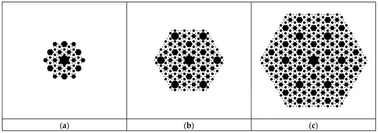
Figure 1. Increasing domain (i.e., number of triangular grid-point located settlements, n), six-tier urban place population directly proportional to graduated filled circle sizes—Christaller K = 3 central place landscapes within a fixed geographic region extent. Left (a) n = 127 (too-small n purges Tier 5). Middle (b): n = 397. Right (c): n = 919.

Table 1. MESF NB specifications for purely contiguous SA latent in Christallerian K = 3 central place geographic distributions of population.

n	Moran Eigenvector Spatial Filters							NB Dispersion Parameter		Residual H0 Probability ⸸
	Positive SA †			Negative SA †			Pseudo-R2
	# of Vectors	ESF zMC	ESF zGR	# of Vectors	ESF |zMC|	ESF zGR		SA	no SA	zMC	zGR
127	0 (34)	N/A	N/A	4 (64)	8.9	3.7	0.85	1.73	0.32	0.2	1.9
271	1 (70)	15.5	6.0	8 (136)	12.3	4.6	0.81	1.77	0.43	0.3	4.0
331	1 (83)	19.5	7.4	9 (165)	14.5	5.7	0.93	1.64	0.23	−0.1	−0.7
397	2 (103)	20.3	7.3	12 (199)	15.9	6.8	0.91	1.50	0.16	0.2	0.5
919	3 (238)	20.4	10.6	11 (468)	25.8	10.4	0.85	1.18	0.20	−0.1	0.8

NOTE: # and N/A respectively denote number and “not applicable”; candidate eigenvector counts in parentheses. ^† the nature of each selected vector; z_MC and z_GR denote the z-scores of the MC and the GR. ⸸ bold font denotes the presence of statistically significant SA.

Autoregressive models provided the first SA tools that were more sophisticated than basic quantitative indices solely gauging the nature and degree of SA, such as the MC and GR reported in Table 1. These were among the original innovative statistics that launched SA hypothesis testing. Their primary weakness is that their only truly successful specification is the auto-normal model, restricting spatial analysis to a normal curve theory inferential foundation even after its golden age came to an end in the 1970s. One major advantage of MESF is that it overcomes this obstacle, supplying an alternative SA tool capable of properly executing non-normal data analyses. Kindred autoregressive instruments include the MC and the Moran scatterplot. Table 2 tabulates, and Figure 2 portrays, these specific renditions of this generic SA tool category. Table 2 results corroborate those summarized in Table 1: K = 3 central place population distributions exhibit a positive-negative SA mixture in which negative SA dominates. Figure 2 reinforces this impression: the Moran scatterplots almost exclusively picture negative SA (i.e., clouds of points—comprising only five or six distinct tier-related quantities—concentrate in the second and fourth quadrants of the graph). Table 2 and Figure 2 also highlight that autoregression can be an inferior tool (e.g., S-W strongly implies non-normal data, the data type for counts, and the multiplicity of point values dramatically diminishes the scatterplot spread, suggesting markedly reduced conventional information content). In other words, the availability of a suite of distinctive SA tools helps spatial analysts tune into delicate intricacies and discerning features of a georeferenced dataset, revealing map pattern aspects that may be elusive to probes by one of these methods alone.

Table 2. SA estimation: two-parameter auto-normal approximation.

n	LN (Population + ő)				SARMA SA Parameters			Pseudo-R2	Residuals
	ő	S-W †	zMC	−zGR	SAR: $\widehat{\mathsf{\rho }}$	${\mathbf{r}}_{\widehat{\mathsf{\rho }}\widehat{\mathsf{\vartheta }}}$	−MA: $-\widehat{\mathsf{\theta }}$		zMC	−zGR
127	0.0	0.65	−5.5	−1.5	−1.71	0.91	1.10	0.775	−0.3	0.5
271	0.0	0.63	−7.9	−1.6	−1.81	0.72	1.38	0.772	−0.7	1.5
331	0.2	0.62	−10.0	−4.4	−1.75	0.87	1.26	0.739	−1.2	−1.1
397	0.0	0.62	−11.5	−4.9	−1.80	0.74	1.39	0.707	−1.4	−1.2
919	0.0	0.64	−18.6	−7.6	−1.84	0.55	1.42	0.672	−2.4	−1.6

^† S-W denotes the Shapiro–Wilk normality diagnostic statistic, whose target value is 1. NOTE: Because the GR and the MA parameter θ have inverse relationships with negative SA, they have been multiplied by −1; none of the parameter correlations are problematic.

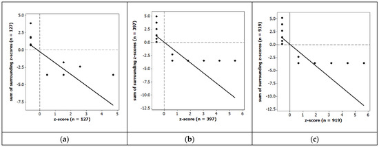
Figure 2. Moran scatterplots for selected Figure 1 central place landscape city populations, revealing only high-low and low-high LISA (signifying negative SA); solid black straight lines denote MC trendlines. Left (a): n = 127. Middle (b): n = 397. Right (c): n = 919.

The third prominent general SA tool applied in this georeferenced data analysis example, namely the semivariogram model, comes from geostatistics and is closely aligned with the GR index: a GR correlogram tends to mimic a semivariogram plot. Of note is that engineering a Geary eigenvector spatial filtering SA tool is feasible, but proves to be inferior to its MESF opponent, which, as its eponymous name proclaims, relates to the MC and the Moran scatterplot. As an enlightening aside, Borcard et al. [78,79] exploit relationships between geostatistics and MESF. Meanwhile, the most appropriate semivariogram model for central place landscapes is the wave-hole (aka hole effect, oscillating, and periodic) specification (e.g., [80,81]). This SA instrument is uniquely suitable for capturing contrasts between neighboring triangular grid location attribute values, making it ideal for central place datasets exhibiting both positive and negative SA. Unlike standard monotonic models (e.g., spherical, exponential, K Bessell), which assume exclusively positive spatial dependence/correlation, and therefore cannot represent negative SA, this wave-hole model accommodates periodic oscillations in semivariance materializing after a relatively short-distance positive SA radius. Rising semivariance over relatively small lag distances that approaches a sill reflects similarity among nearby values (i.e., positive SA), whereas the subsequent characteristic troughs/holes indicate larger separation distances at which higher-order nearest neighbors are systematically dissimilar (i.e., negative SA). The wavelength parameter (e.g., see Table 3) in this model specifies the geographic scale at which these sign changes occur, enabling a precise description of alternating map patterns embedded in spatial structure. Fitting a wave-hole model when negative SA dominates can quantify both the strength of local contrasts and the scale of geographic fluctuation, providing a coherent framework for spatial prediction, simulation, and SA inference in geographic landscapes where negative SA meaningfully organizes their georeferenced data. When positive SA dominates in such mixture scenarios, the wave-hole model becomes part of a valid linear combination ([82], p. 24) that also includes a specification emphasizing positive SA (e.g., the K Bessell). Nevertheless, Figure 3 demonstrates that geostatistical analysis here is deficient. Only the n = 127 case exposes an appropriate wave-hole description, although all three graphics exhibit some amount of oscillation. Table 3 records a non-zero nugget for the other four cases, and autonomous deductions that each fails to generate an eloquent cross-tabulation scatterplot.

Table 3. Estimated wave-hole semivariogram model parameters.

n	Nugget	Sill	Range/Wavelength	RMSE †	Cross-Validation
127	0	472	1.95	25.9	linear trend entirely absent
271	271	92	8.96	19.9	linear trend entirely absent
331	246	53	9.85	17.9	linear trend entirely absent
397	215	36	10.77	16.3	linear trend entirely absent
919	111	11	4.02	11.3	linear trend entirely absent

^† RMSE denotes root mean squared error.

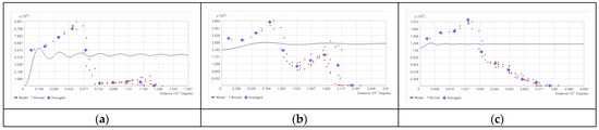
Figure 3. Estimated wave-hole model plots superimposed on empirical semivariograms for Figure 1 central place populations. Left (a): n = 127. Middle (b): n = 397. Right (c): n = 919.

As the showcased empirical example documents, the spatial structure concept plays a central role in clarifying map pattern relationships implanted in geospatial datasets, aligning directly with the framing introduced earlier in this paper. Spatial structure provides the observable form through which SA becomes manifest within theoretical constructs as well as geotagged data. Whether expressed as gradients, clusters, contrasts, hierarchies, or networks, spatial structure represents the patterned outcome of spatial dependence/correlation operating within theoretical and contextual geographical landscape constraints. In this sense, emphasized by the immediately prior SA tools output, spatial structure should not be viewed as a parallel or ancillary concern, but rather as the mechanism through which spatial dependence/correlation is rendered visible, interpretable, and theoretically meaningful. Aligning spatial structure with SA strengthens coherence between geographic theory, real-world empirical observation, and spatial statistical inference. Methodologically, a wide range of analytical approaches—such as the preceding proximity indices, MESF, lattice-based autoregressive models, and geostatistical techniques—operationalize SA as a data analytic tool in different ways, depending upon georeferenced data type, scale, and/or research objectives. These approaches differ in implementation, but collectively they function as lenses for revealing spatial structure rather than as substitutes for the theoretical assumptions that give rise to spatial dependence/correlation. Taken together, these contentions and empirical analyses suggest that SA occupies a dual role within geographic inquiry: it routinely is generated by spatial processes embedded in theory, yet often is rendered latent by the very constraints that make theory operational. This tension helps explain both the ubiquity of SA across geographic domains and its relative invisibility in theoretical discourse. Recognizing this duality motivates a more explicit engagement with SA’s conceptual implications, which forms the basis of the call to action outlined in this paper.

Therefore, the takeaway here is that jointly explicating SA dependency/correlation in theories and SA correlation artifacts via methodology establishes a coherent route from conceptual establishment to coordinated adoption. Theories become more realistic. Empirical analyses become more accurate and robust. Qualitative insights become geographically regulated. Spatial sampling designs become more defensible, efficient, and repeatable, replicable, and reproducible because of simple random sampling corruption by SA (e.g., [83]), a viewpoint aggressively disputed by some (e.g., [84]). SA emerges not merely as a statistical afterthought, but rather as a unifying principle linking together the intellectual architectures of human and physical/environmental geography, cartographic, and spatial sampling theories. By embracing SA as a core property, when suitable, as opposed to strictly an anomaly to correct (e.g., see [85,86]), geospatial scholars stand to expand the explanatory power, methodological coherence, and cross-subfield and cognate field integration of the discipline’s epistemology and analytic toolkit. This latter collection presently comprises three distinct techniques capable of factoring in SA. The hypothetical central place example in this section ranks them as follows: (1) MESF is preferable; (2) autoregression is marginally acceptable; and (3) geostatistics is somewhat unhelpful. In contrast, if this illustration concerned physical geography digital elevation model (DEM [63], Ch. 3) or soil (e.g., [87,88,89,90]) elements, the ranking almost certainly would be: (1) geostatistics is preferable; (2) MESF is marginally acceptable; and, (3) autoregression most likely is unhelpful (e.g., see [76]).

8. Concluding Comments, Implications, and Some Future Research

This paper demonstrates that SA is neither a peripheral statistical curiosity/inconvenience nor a methodological spatial data property nuisance. Instead, it constitutes a structurally embedded and theoretically consequential feature of virtually all georeferenced phenomena that has long shaped explanation, representation, and inference across the discipline. Surprisingly and lamentably, it has been largely overlooked—suffering a form of inattentional blindness—in geographic theories to date. SA governs the distribution of too-often falsely assumed independent information across space, shaping quantitative postulates and sampling efficiency, qualitative saturation, and the interpretive reach of humanistic inquiries. Throughout human, physical, and cartographic geography theories, the presence of SA fundamentally constrains how landscapes are represented, analyzed, and understood, linking proximate observations via latent dependencies/correlations while revealing map patterns that frequently are masked in naïve geospatial data examinations.

8.1. Implications

The recognition of SA as a common ingredient in spatial constructs carries profound theoretical, methodological, and empirical implications. Conceptually, it reframes the understanding of geographic trends and processes: nearby locations are rarely independent, and spatial dependencies/correlations mediate diffusion, persistence, and regional coherence across geographic scales and resolutions. Ignoring SA risks misrepresenting variation, inflating apparent precision, and overlooking the underlying spatial logic that unites diverse geographic phenomena—from settlement hierarchies to environmental gradients to cultural clustering to spatial interpolation.

Methodologically, SA underscores the necessity of explicitly spatially informed devices and analyses. Quantitative studies benefit from SA-exploiting data collection by way of tessellation-stratified random sampling, variogram-based kriging instituted upon a carefully crafted geographic landscape coverage by sample points, and MESF to exploit mimicked independent information, adequately address the seemingly universal positive-negative SA mixtures where negative SA should be interpreted as informative contrasts rather than pathological artifacts (e.g., [91]), and optimize inferential accuracy. Qualitative and mixed-method approaches gain from awareness of spatial structuring in sample selection and saturation assessments, ensuring that culturally, socially, and ecologically meaningful variation is adequately encapsulated. Together, these approaches elevate methodological rigor, reduce redundancy, and enhance interpretive credibility and trustworthiness across the discipline of geography.

Empirically, SA’s pervasiveness is evident across canonical and contemporary exemplifications. For example, from Christaller-style central place hierarchies to the Asheville, NC, Southern Highland Craft Guild network in human geography, from DEM-based terrain surfaces to soil attribute distributions in physical geography, and from proper design-based quantitative evidence gathering to census-driven racial identity patterns in spatial sampling, SA shapes the very fabric of geospatial reality. Accounting for SA allows geospatial researchers to reveal previously obscured geographic heterogeneity, improve predictive modeling, and generate robust, repeatable/reproducible/replicable empirical evidence and findings.

8.2. A Call to Action

Arguments developed in this paper transmit a need for more explicit engagement with SA across geographic research. First, geographic theorists need to be encouraged to identify explicitly how SA is induced and absorbed within theoretical frameworks. Doing so clarifies the spatial logic underlying core assumptions and strengthens theory testing by distinguishing expected structure from unexplained dependence and artifactual correlation. Second, spatial analysts and quantitative modelers need to treat residual SA not solely as a specification problem to be corrected, but also as a potentially informative signal of missing covariates, scale mismatches, and/or theoretical incompleteness. In particular, mixtures of positive and negative spatial dependence/correlation may encode meaningful geographic contrasts that warrant interpretation rather than automatic correction.

Meanwhile, researchers working in qualitative, interpretive, and place-based traditions may benefit from recognizing how spatial structuring underlies clustering, differentiation, and experiential coherence. Explicit awareness of SA can strengthen case selection, interpretation, and spatial grounding without constraining methodological pluralism. Finally, educators and methodologists need to be encouraged to integrate SA more fully into geographic training, treating it as a foundational conceptual principle rather than a specialized technical topic. Such integration will better equip future geographers to design spatially robust studies, and to render critical interpretations of patterned geographic variation.

Looking forward, further work, as detailed in the next subsection, should explore multiscale, anisotropic, and nonstationary forms of SA, among other topics, revisit additional geographic theories through an explicitly SA-informed lens, and continue to bridge theory, data, and method. Making SA explicit transforms it from an unspoken assumption into a central component of geographic inquiry—one that enriches theory, sharpens inference, and strengthens coherence across the discipline.

8.3. Future Research

Building upon the foundation this paper erects, several avenues merit further attention. First, and foremost, refinement and expansion of all spatial theories, supplementing those dissected in this paper, is essential. Efforts to capture multiscale, anisotropic, and nonstationary spatial processes (e.g., [92]), as well as temporal evolution of spatial dependence/correlation, will enhance theoretical fidelity and empirical relevance. Integrating SA into predictive frameworks, including machine learning and network-based approaches, represents a frontier for SA in the context of spatially aware analytics.

Second, conceptual elaboration of SA remains critical. Clarifying the mechanisms underpinning positive, negative, and their mixtures of SA, and linking these patterns explicitly to diffusion, segregation, optimization, and hierarchical processes, among other themes, will strengthen the explanatory power of geographic theories. This conceptual refinement also will support cross-subfield dialog, bridging quantitative, qualitative, and geohumanities traditions under a coherent spatial framework.

Third, pedagogical and functional integration is imperative. Developing instructional materials, reproducible workflows, and software tools that foreground SA as a core principle will cultivate a new generation of quantitative and qualitative geographers alike who are capable of designing more spatially robust studies. Likewise, codifying SA-aware best practices in sampling, modeling, and visualization will ensure consistent methodological adoption across applied and theoretical geospatial domains.

Finally, interdisciplinary engagement offers additional fertile opportunities. As spatial data proliferate in criminology, demography, economics, environmental management, public health, urban planning, and other medical, natural, and social sciences, explicit incorporation of SA will enhance cognate inference, improve decision-making, and clarify spatial mechanisms in complex, coupled human–environment interactions and systems.

In conclusion, bringing SA to the forefront transforms it from a latent statistical property to a unifying, operationally central principle in geography. Embracing SA enriches theoretical coherence, strengthens methodological integrity, and amplifies empirical insight, providing a durable foundation for future research across geography’s human, physical, cartographic, and methodological horizons. Many geographic theories afford fertile topics for inquiry because they still have not been demystified through a SA prism!

References

- Tobler, W.R. A computer movie simulating urban growth in the Detroit region. Econ. Geogr. 1970, 46, 234–240. [Google Scholar] [CrossRef]
- Griffith, D.A.; Chun, Y.; Kim, H. Spatial autocorrelation informed approaches to solving location–allocation problems. Spat. Stat. 2022, 50, 100612. [Google Scholar] [CrossRef]
- Griffith, D. Spatial autocorrelation is everywhere—Even in poetry. GeoHumanities 2025. forthcoming. [Google Scholar]
- Griffith, D.; Li, B. Spatial Autocorrelation: A Fundamental Property of Geospatial Phenomena; Elsevier: Amsterdam, The Netherlands, 2025. [Google Scholar]
- Griffith, D.; Layne, L. Uncovering relationships between geo-statistical and spatial autoregressive models. In 1996 Proceedings on the Section on Statistics and the Environment; American Statistical Association: Alexandria, VA, USA, 1997; pp. 91–96. [Google Scholar]
- Griffith, D.; Fischer, M.; LeSage, J. The spatial autocorrelation problem in spatial interaction modelling: A comparison of two common solutions. Lett. Spat. Resour. Sci. 2017, 10, 75–86. [Google Scholar] [CrossRef]
- Lee, C.; Griffith, D.A.; Chun, Y.; Kim, H. Effects of geographically stratified random sampling initial solutions on solving a continuous surface p-median location problem using the ALTERN heuristic. Spat. Stat. 2023, 57, 100768. [Google Scholar] [CrossRef]
- Kim, H.; Chun, Y.; Griffith, D. An efficient solution approach for the p-median problems with spatially autocorrelated weights. Ann. Am. Assoc. Geogr. 2025. forthcoming. [Google Scholar]
- Sen, A.; Smith, T. Gravity Models of Spatial Interaction Behavior; Springer: Berlin/Heidelberg, Germany, 1995. [Google Scholar]
- O’Sullivan, D.; Unwin, D. Geographic Information Analysis; Wiley: Hoboken, NJ, USA, 2010. [Google Scholar]
- Assunção, R.M.; Neves, M.C.; Câmara, G.; Da Costa Freitas, C. Efficient regionalization techniques for socio-economic geographical units using minimum spanning trees. Int. J. Geogr. Inf. Sci. 2006, 20, 797–811. [Google Scholar] [CrossRef]
- Hägerstrand, T. Innovation Diffusion as a Spatial Process; University of Chicago: Chicago, IL, USA, 1967. [Google Scholar]
- Gould, P. Spatial Diffusion; Resource Paper No. 4; American Association of Geographers: Washington, DC, USA, 1969. [Google Scholar]
- Blaikie, P. The theory of the spatial diffusion of innovations: A spacious cul-de-sac. Prog. Hum. Geogr. 1978, 2, 268–295. [Google Scholar] [CrossRef]
- Cliff, A.; Ord, J. Spatial Autocorrelation; Pion: London, UK, 1973. [Google Scholar]
- Morrill, R.; Gaile, G.; Thrall, G. Spatial Diffusion; SAGE: Thousand Oaks, CA, USA, 1988. [Google Scholar]
- Valente, T.W.; Yon, G.G.V. Diffusion/contagion processes on social networks. Health Educ. Behav. 2020, 47, 235–248. [Google Scholar] [CrossRef]
- Bokányi, E.; Novák, M.; Jakobi, Á.; Lengyel, B. Urban hierarchy and spatial diffusion over the innovation life cycle. R. Soc. Open Sci. 2022, 9, 211038. [Google Scholar] [CrossRef]
- Griffith, D. Spectral geometry and Riemannian manifold mesh approximations: Some autocorrelation lessons from spatial statistics. J. Math. Arts 2023, 17, 293–313. [Google Scholar] [CrossRef]
- Griffith, D.A. Getis’s spatial filtering legacy: Spatial autocorrelation mixtures in geospatial agricultural datasets. J. Spat. Econ. 2023, 4, 1–33. [Google Scholar] [CrossRef]
- Griffith, D. Spatial autocorrelation and central place theory. Cybergeo 2025. under review. [Google Scholar]
- Stoddart, D. Historical geography of physical geography. In Directions in Geography; Chorley, R., Ed.; Methuen: London, UK, 1975; pp. 57–78. [Google Scholar]
- Gurnell, A. Twenty-five years of progress in physical geography: A personal view of its antecedents and trajectory. Geography 2018, 103, 122–136. [Google Scholar] [CrossRef]
- Descombes, P.; Leprieur, F.; Albouy, C.; Heine, C.; Pellissier, L. Spatial imprints of plate tectonics on extant richness of terrestrial vertebrates. J. Biogeogr. 2017, 44, 1185–1197. [Google Scholar] [CrossRef]
- Moustafa, S.; Yassien, M.; Metwaly, M.; Faried, A.; Elsaka, B. Applying geostatistics to understand seismic activity patterns in the Northern red sea boundary zone. Appl. Sci. 2024, 14, 1455. [Google Scholar] [CrossRef]
- Leighly, J. Climatology since the year 1800. Eos 1949, 30, 658–672. [Google Scholar]
- Mock, C. Climatology: History. In International Encyclopedia of Geography; Richardson, D., Castree, N., Goodchild, M., Kobayashi, A., Liu, W., Marston, R., Eds.; Wiley: Hoboken, NJ, USA, 2016; pp. 1–5. [Google Scholar] [CrossRef]
- Winkler, J. Climatology. In The International Encyclopedia of Geography; Richardson, D., Castree, N., Goodchild, M., Kobayashi, A., Liu, W., Marston, R., Eds.; Wiley: Hoboken, NJ, USA, 2017; pp. 1–12. [Google Scholar] [CrossRef]
- Mauelshagen, F. Climate as a scientific paradigm—Early history of climatology to 1800. In The Palgrave Handbook of Climate History; White, S., Pfister, C., Mauelshagen, F., Eds.; Palgrave Macmillan: London, UK, 2018; pp. 565–588. [Google Scholar]
- Kottek, M.; Rubel, F. Global daily precipitation fields from bias-corrected rain gauge and satellite observations. Part I: Design and development. Meteorol. Z. 2007, 16, 525–540. [Google Scholar] [CrossRef]
- Hutton, J. Theory of the Earth; or an Investigation of the Laws Observable in the Composition, Dissolution, and Restoration of Land upon the Globe. Trans. R. Soc. Edinb. 1788, 1, 209–304. [Google Scholar] [CrossRef]
- Sauer, F.; Uthmeier, T. Geomorphological diversity and habitat variability. A model of late Palaeolithic catchment composition in Northern Bavaria: Geomorphologische diversität und habitatvariabilität. Ein modell der spätpaläolithischen catchment in Nordbayern. Quartär—Int. Jahrb. Erforsch. Eiszeitalt. Steinzeit 2020, 67, 85–103. [Google Scholar]
- Kim, D.; Šamonil, P.; Jeong, G.; Tejnecký, V.; Drábek, O.; Hruška, J.; Park, S. Incorporation of spatial autocorrelation improves soil–landform modeling at A and B horizons. Catena 2019, 183, 104226. [Google Scholar] [CrossRef]
- Jenny, H. Factors of Soil Formation: A System of Quantitative Pedology; Dover: Dutchess, NY, USA, 1941. [Google Scholar]
- Robinson, A. The genealogy of the isopleth. Cartogr. J. 1971, 8, 49–53. [Google Scholar] [CrossRef]
- Friendly, M. The golden age of statistical graphics. Stat. Sci. 2008, 23, 502–535. [Google Scholar] [CrossRef]
- Monmonier, M. Air Apparent: How Meteorologists Learned to Map, Predict, and Dramatize Weather; University of Chicago Press: Chicago, IL, USA, 2000. [Google Scholar]
- Wu, X.; Zurita-Milla, R.; Kraak, M. Visual discovery of synchronisation in weather data at multiple temporal resolutions. Cartogr. J. 2013, 50, 247–256. [Google Scholar] [CrossRef]
- Snyder, J. Flattening the Earth: Two Thousand Years of Map Projections; University of Chicago Press: Chicago, IL, USA, 1997. [Google Scholar]
- Bertin, J. Sémiologie Graphique: Les Diagrammes, les Réseaux, les Cartes (Semiology of Graphics: Diagrams, Networks, Maps); Berg, W., Translator; Esri Press: Redlands, CA, USA, 2010. [Google Scholar]
- Tolman, E. Cognitive maps in rats and men. Psychol. Rev. 1948, 55, 189–208. [Google Scholar] [CrossRef]
- Golledge, R.; Jacobson, R.; Kitchin, R.; Blades, M. Cognitive maps, spatial abilities and human wayfinding. Geogr. Rev. Jpn. Ser. B. 2000, 73, 93–104. [Google Scholar]
- Gould, P.; White, R. Mental Maps, 2nd ed.; Routledge & Kegan Paul: Ithaca, NY, USA, 1986. [Google Scholar]
- Christaller, W. Die Zentralen Orte in Süddeutschland: Eine Ökonomisch-Geographische Untersuchung Über die Gesetzmäßigkeit der Verbreitung und Entwicklung der Siedlungen mit Städtischen Funktionen (Central Places in Southern Germany); Gustav Fischer: Jena, Germany, 1933. [Google Scholar]
- Lösch, A. Die Räumliche Ordnung der Wirtschaft, 2nd ed.; Gustav Fischer: Jena, Germany, 1944. [Google Scholar]
- Moran, P. Notes on continuous stochastic phenomena. Biometrika 1950, 37, 17–23. [Google Scholar]
- Geary, R. The contiguity ratio and statistical mapping. Incorp. Stat. 1954, 5, 115–146. [Google Scholar]
- Tomlin, C. Map algebra: One perspective. Landsc. Urban Plan. 1994, 30, 3–12. [Google Scholar] [CrossRef]
- Groves, R.; Fowler, F.; Couper, M.; Lepkowski, J.; Singer, E.; Tourangeau, R. Survey Methodology, 2nd ed.; Wiley: Hoboken, NJ, USA, 2009. [Google Scholar]
- Patton, M. Qualitative Research & Evaluation Methods, 4th ed.; Sage: Thousand Oaks, CA, USA, 2015. [Google Scholar]
- Creswell, J.; Creswell, J. Research Design: Qualitative, Quantitative, and Mixed Methods Approaches, 6th ed.; Sage: Thousand Oaks, CA, USA, 2022. [Google Scholar]
- Griffith, D.; Plant, R. Statistical analysis in the presence of spatial autocorrelation: Selected sampling strategy effects. Stats 2022, 5, 1334–1353. [Google Scholar] [CrossRef]
- Guillot, G.; Leblois, R.; Coulon, A.; Frantz, A. Statistical methods in spatial genetics. Mol. Ecol. 2009, 18, 4734–4756. [Google Scholar] [CrossRef]
- Olsson, G. Explanation, prediction, and meaning variance: An assessment of distance interaction models. Econ. Geogr. 1970, 46, 223–233. [Google Scholar] [CrossRef]
- Cliff, A.; Ord, J. The problem of spatial autocorrelation. In London Papers in Regional Science 1, Studies in Regional Science; Scott, A., Ed.; Pion: London, UK, 1969; pp. 25–55. [Google Scholar]
- Cressie, N. Statistics for Spatial Data; Wiley: Hoboken, NJ, USA, 1993. [Google Scholar]
- Legendre, P. Spatial autocorrelation: Trouble or new paradigm? Ecology 1993, 74, 1659–1673. [Google Scholar] [CrossRef]
- Bailey, T.; Gatrell, A. Interactive Spatial Data Analysis; Longman Scientific & Technical: Harlow, UK, 1995. [Google Scholar]
- Haining, R. Spatial Data Analysis: Theory and Practice; Cambridge University Press: Cambridge, UK, 2003. [Google Scholar]
- Griffith, D. Art, geography/GIScience, and mathematics: A surprising interface. Ann. Assoc. Am. Geogr. 2023, 113, 1–12. [Google Scholar] [CrossRef]
- Acosta, J.; Vallejos, R.; Griffith, D. On the effective geographic sample size. J. Stat. Comput. Simul. 2018, 88, 1958–1975. [Google Scholar] [CrossRef]
- Webster, R.; Oliver, M. Geostatistics for Environmental Scientists, 2nd ed.; Wiley: Hoboken, NJ, USA, 2007. [Google Scholar]
- Chun, Y.; Griffith, D. Spatial Statistics & Geostatistics; SAGE: Thousand Oaks, CA, USA, 2013. [Google Scholar]
- Griffith, D. Effective geographic sample size in the presence of spatial autocorrelation. Ann. Am. Assoc. Geogr. 2005, 95, 740–760. [Google Scholar] [CrossRef]
- Schelling, T. Models of segregation. Am. Econ. Rev. 1969, 59, 488–493. [Google Scholar]
- Schelling, T. Dynamic models of segregation. J. Math. Sociol. 1971, 1, 143–186. [Google Scholar] [CrossRef]
- Cliff, A.; Ord, J. Spatial Processes: Models & Applications; Pion: London, UK, 1981. [Google Scholar]
- Openshaw, S. A geographical solution to scale and aggregation problems in region-building, partitioning and spatial modelling. Trans. Inst. Br. Geogr. 1977, 2, 459–472. [Google Scholar] [CrossRef]
- Hartshorne, R. The concept of geography as a science of space, from Kant and Humboldt to Hettner. Ann. Assoc. Am. Geogr. 1958, 48, 97–108. [Google Scholar] [CrossRef]
- Hill, M. Positivism: A ‘hidden’ philosophy in geography. In Themes in Geographic Thought; Harvey, M., Holly, B., Eds.; Croom Helm: London, UK, 1981; pp. 38–60. [Google Scholar]
- Goodchild, M. Questions, tools or paradigms: Scientific geography in the 1980s. Ont. Geogr. 1985, 25, 3–14. [Google Scholar]
- Martin, G. American Geography and Geographers; Toward Geographical Science: Oxford, NY, USA, 2015. [Google Scholar]
- Agbebaku, H. A review of the evolution of geography from non-science to science discipline since the history of geographic thought. West Afr. J. Open Flex. Learn. 2020, 9, 103–122. [Google Scholar]
- Kourtit, K.; Nijkamp, P.; Suzuki, S. The science of space: New endeavours in regional science. Asia-Pac. J. Reg. Sci. 2021, 5, 149–153. [Google Scholar] [CrossRef]
- Griffith, D.; Fischer, M. Constrained variants of the gravity model and spatial dependence: Model specification and estimation issues. J. Geogr. Syst. 2013, 15, 291–317. [Google Scholar] [CrossRef]
- Cressie, N.; Kaiser, M.; Daniels, M.; Aldworth, J.; Lee, J.; Lahiri, S.; Cox, L. Spatial analysis of particulate matter in an urban environment. In Proceedings of the geoENV II—Geostatistics for Environmental Applications Proceedings, Second European Conference on Geostatistics for Environmental Applications, Valencia, Spain, 18–20 November 1998; Gómez-Hernández, J., Soares, A., Froidevaux, R., Eds.; Springer: Dordrecht, The Netherlands, 1999; pp. 41–52. [Google Scholar]
- Griffith, D.; Li, B.; Millones, M.; Injoque, F.; Quispe, B.; Villarino, A. A second spatial autocorrelation mechanism: Geographic hierarchies and urban systems. Glob. Chall. Reg. Sci. 2025, 4, 100022. [Google Scholar] [CrossRef]
- Borcard, D.; Legendre, P. All-scale spatial analysis of ecological data by means of principal coordinates of neighbour matrices. Ecol. Model. 2002, 153, 51–68. [Google Scholar] [CrossRef]
- Borcard, D.; Legendre, P.; Avois-Jacquet, C.; Tuomisto, H. Dissecting the spatial structure of ecological data at multiple scales. Ecology 2004, 85, 1826–1832. [Google Scholar] [CrossRef]
- Journel, A.; Froidevaux, R. Anisotropic hole-effect modeling. Math. Geol. 1982, 14, 217–239. [Google Scholar]
- Pyrcz, M.; Deutsch, C. The Whole Story on the Hole Effect; Searston, S., Ed.; Newsletter 18; Geostatistical Association of Australasia: West Perth, Australia, 2003; 16p, Available online: https://ccg-server.engineering.ualberta.ca/CCG%20Publications/Other/CVD%20Papers/02-Conference/2003/holeEffectpaper.pdf (accessed on 5 February 2026).
- Deutsch, C.; Journel, A. GSLIB: Geostatistical Software Library and User’s Guide, 2nd ed.; Oxford University Press: New York, NY, USA, 1998. [Google Scholar]
- Griffith, D. Establishing qualitative geographic sample size in the presence of spatial autocorrelation. Ann. Assoc. Am. Geogr. 2013, 103, 1107–1122. [Google Scholar] [CrossRef]
- Brus, D. Statistical approaches for spatial sample survey: Persistent misconceptions and new developments. Eur. J. Soil Sci. 2021, 72, 686–703. [Google Scholar] [CrossRef]
- Cliff, A. Quantitative methods: Spatial diffusion. Prog. Hum. Geogr. 1979, 3, 143–152. [Google Scholar] [CrossRef]
- Goodchild, M. What problem? Spatial autocorrelation and geographic information science. Geogr. Anal. 2009, 41, 411–417. [Google Scholar] [CrossRef]
- Burgess, T.; Webster, R. Optimal interpolation and isarithmic mapping of soil properties: I The semi-variogram and punctual kriging. J. Soil Sci. 1980, 31, 315–331. [Google Scholar] [CrossRef]
- Goovaerts, P. Geostatistics in soil science: State-of-the-art and perspectives. Geoderma 1999, 89, 1–45. [Google Scholar] [CrossRef]
- Lark, R. Towards soil geostatistics. Spat. Stat. 2012, 1, 92–99. [Google Scholar] [CrossRef]
- Heuvelink, G.; Webster, R. Spatial statistics and soil mapping: A blossoming partnership under pressure. Spat. Stat. 2022, 50, 100639. [Google Scholar] [CrossRef]
- Hu, L. Negative Spatial Autocorrelation and Its Impacts on Georeferenced Data Analyses: With Case Studies of Cancer Incidences. Ph.D. Thesis, University of Texas at Dallas, Richardson, TX, USA, 2020. [Google Scholar]
- Gelfand, A.; Diggle, P.; Guttorp, P.; Fuentes, M. Handbook of Spatial Statistics; CRC: Boca Raton, FL, USA, 2010. [Google Scholar]
Disclaimer/Publisher’s Note: The statements, opinions and data contained in all publications are solely those of the individual author(s) and contributor(s) and not of MDPI and/or the editor(s). MDPI and/or the editor(s) disclaim responsibility for any injury to people or property resulting from any ideas, methods, instructions or products referred to in the content. |
© 2026 by the author. Published by MDPI on behalf of the International Society for Photogrammetry and Remote Sensing. Licensee MDPI, Basel, Switzerland. This article is an open access article distributed under the terms and conditions of the Creative Commons Attribution (CC BY) license.