Article

Urban Air Pollutant Monitoring through a Low-Cost Mobile Device Connected to a Smart Road

1
ENEA, Robotics and AI Laboratory, Casaccia Research Centre, 00123 Rome, Italy
2
ENEA, Analysis and Protection of Critical Infrastructures Laboratory, Casaccia Research Centre, 00123 Rome, Italy
3
EISAC.it, Italian Node of the European Infrastructure Simulation and Analysis Centre, Via di Vigna Murata 651, 00143 Rome, Italy
*
Author to whom correspondence should be addressed.
ISPRS Int. J. Geo-Inf. 2022, 11(2), 132; https://doi.org/10.3390/ijgi11020132
Submission received: 20 January 2022 / Revised: 9 February 2022 / Accepted: 12 February 2022 / Published: 14 February 2022

Abstract

:
Air pollutant monitoring is a basic issue in contemporary urban life. This paper describes an approach based on the diffused use of low-cost sensors that can be mounted on board urban vehicles for more abundant and distributed measures. The system exchanges data, exploiting a “Smart Road” infrastructure, with a central computing facility, the CIPCast platform, a GIS-based Decision Support System designed to perform real-time monitoring and interpolation of data with the aim of possibly issuing alarms with respect to different town areas. Experimental data gathering in the Rome urban area and subsequent processing results are presented. Algorithms for data fusion among different simulated monitoring systems and interpolation of data for a geographically denser map were utilised. Thus, in the framework of the Smart Road, protocols for data exchange were designed. Finally, air pollutant distribution maps were produced and integrated into the CIPCast platform. The feasibility of a full system architecture from the sensors to the real-time pollutant maps is shown.

1. Introduction

Human health is adversely affected by exposure to air pollutants with chronic and long-term ailments ranging from upper respiratory irritation to deadly morbidities such as lung cancer and heart diseases [1]. The underlining cause is represented by the ever-increasing consumption of energy, most of it in the form of the burning of fossil fuels. This produces huge amounts of carbon dioxide (CO2), contributing to the warming of our planet, and, at the same time, outputs a series of air pollutants that have a direct and harmful influence on human health: carbon monoxide (CO), sulphur dioxide (SO2), nitrogen oxides (NOx), and particulate matters of several sizes (PM-1, PM-2.5, and PM-10). In addition, long-term exposure has been linked to premature mortality [2].
This problem has been tackled at a legislative level with the installation of monitoring systems in urban areas. Current systems are usually sparsely distributed in the urban area with a very low spatial resolution. As an example, in the area of Rome there are 13 monitoring stations, managed by ARPA, the Lazio environmental agency [3], of which 10 are inside the “Grande Raccordo Anulare” (GRA, the beltway around the town). If an average radius of 9 km is assumed for the GRA, then each station covers a surface of 25 km2 if evenly distributed. If the whole surface of the municipality is considered (1285 km2), and all the available systems, this figure rises to 99 km2. A similar situation can be found in most large towns around the world, e.g., in Beijing there are 22 stations, each covering 113 km2, and in London there are 14 stations, each covering 112 km2 [4].
The sparseness of the data has produced, as a consequence, a need for estimates of the pollutants in unmeasured areas using a variety of methods, e.g., spatial averaging, nearest neighbour, Inverse Distance Weighting (IDW), Spline interpolation, Kriging, Land-Use Regression (LUR) modelling, dispersion modelling, and neural network methods [4].
In recent years, the availability of smaller pollution sensing devices and the Global Navigation Satellite System (GNSS) have opened the way to small-size mobile systems for the monitoring of air pollutants [5]. This increases the density of data, but it does not solve the sparseness problem, since the mobile measurements are usually performed along the streets or in specific areas. In order to obtain a larger view, the same methods previously developed for the interpolation of data from monitoring stations have been applied also in the case of mobile air pollution data [4].
The aim of this paper is to describe an air pollutant monitoring system composed of three different elements: a mobile small-sized device accommodating low-cost sensors (LCSs), a road infrastructure for the communication of data (the Smart Road), and a central computing facility [6]. The sensing device can be easily carried by vehicles in the urban area, e.g., private cars, mass transport buses, and municipality service vehicles. In this work, we analysed the case where several LCSs are geographically dispersed in an urban environment, collecting air quality data and relaying them to an urban centralised processing platform. The communication backbone is furnished by an intelligent infrastructure, namely a Smart Road (SR), which, among other capabilities, can convey the collected data to the central computing facility. This runs a GIS-based Decision Support System (DSS), called Critical Infrastructures Protection risk analysis and foreCAST (CIPCast), designed to perform real-time monitoring, processing, and interpolation of data with the aim of possibly issuing alarms with respect to different areas of the town [7].
In the following, the system is described using the AlphaSense OPC-N2, a well-known and reliable LCS for particulate data. Besides its good features, the particulate concentration is one of the key parameters for the monitoring of air quality and the consequent possibility of reducing or completely eliminating vehicular traffic in urban zones.
Geovisualisation techniques can provide information about various and heterogenous spatial data in an integrated and visual way, allowing us to analyse and better understand environmental phenomena and dynamics [8,9]. In particular, the use of a GIS-based DSS opens the way to a friendly interaction with the particulate data collected in the urban area. It allows us, as an example, to display the historical series in a given location or inspect other relevant geographical information in the area in an interactive way as in [9,10]. The DSS can also effectively support GIS multicriteria decision analysis (MCDA) techniques and Analytic Hierarchy Process (AHP)-based techniques in order to allow for the visualisation and interpretation of the spatial distribution of air pollution impacts [11]. In other approaches [12], GIS-based applications were used to support the best siting of monitoring networks and the qualitative assessment of their spatial representativeness of pollutant emissions and variability. Finally, 3D methods can improve the visualisation capabilities and allow us to assess diffusion by calculating visible and obstructed volumes [13].
In Section 2, the different parts composing the overall system are described. In particular, in the first subsection the LCSs are illustrated with a particular focus on the sensor used in this work. In the second subsection, the features of the SR and the ones relevant to the air monitoring task are described. In the third subsection, the GIS-based CIPCast system is described. A preliminary sensor characterisation is presented in the fourth subsection. In the fifth subsection, the data acquisition campaign is described, and in the sixth subsection the data processing centrally performed in the GIS-based DSS is explained.
In Section 3, the results of these activities are reported. In Section 4, a brief discussion is provided, and in Section 5 our conclusions and some comments are given together with future research directions.

2. Materials and Methods

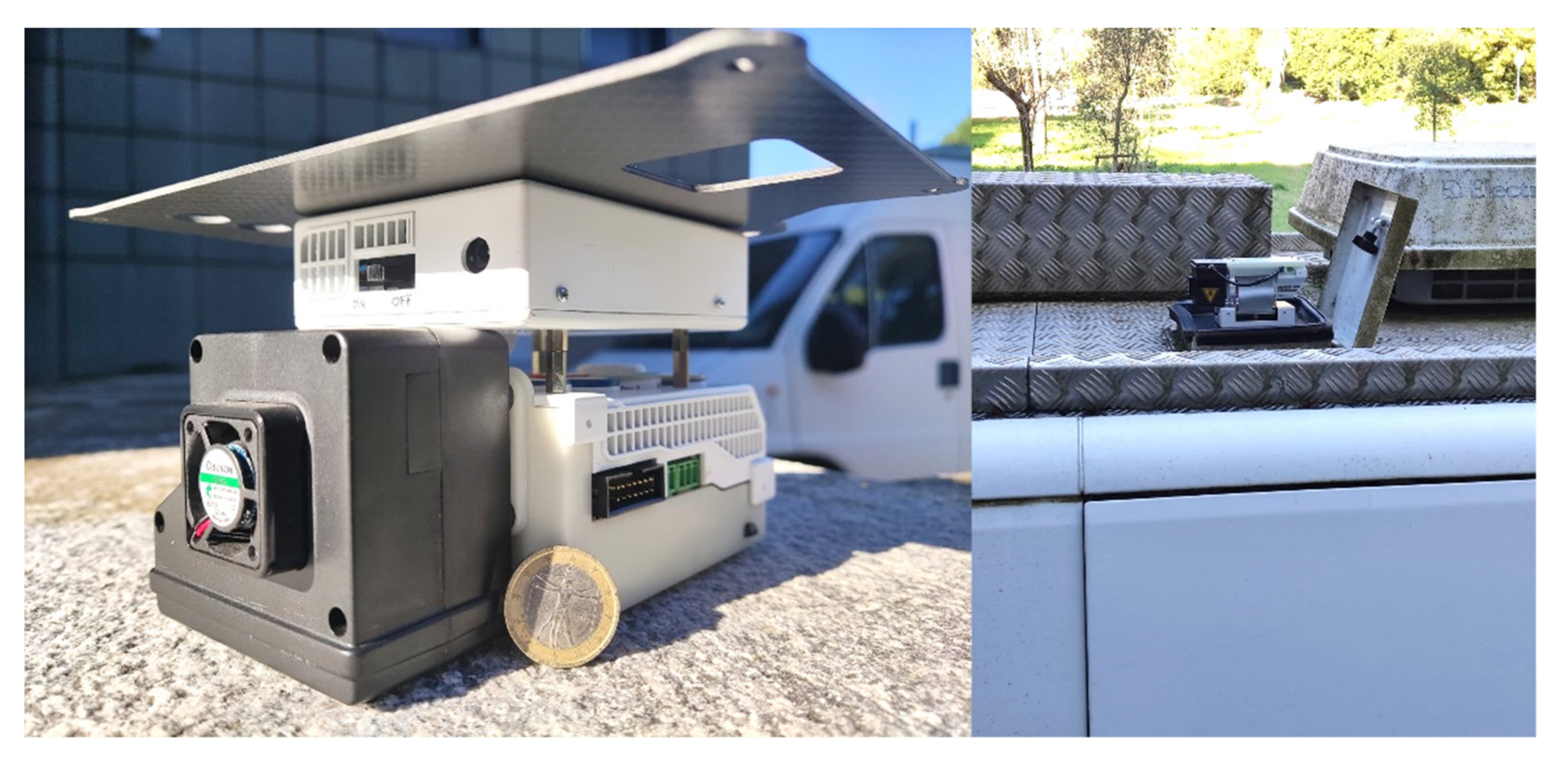
2.1. Low-Cost Sensors
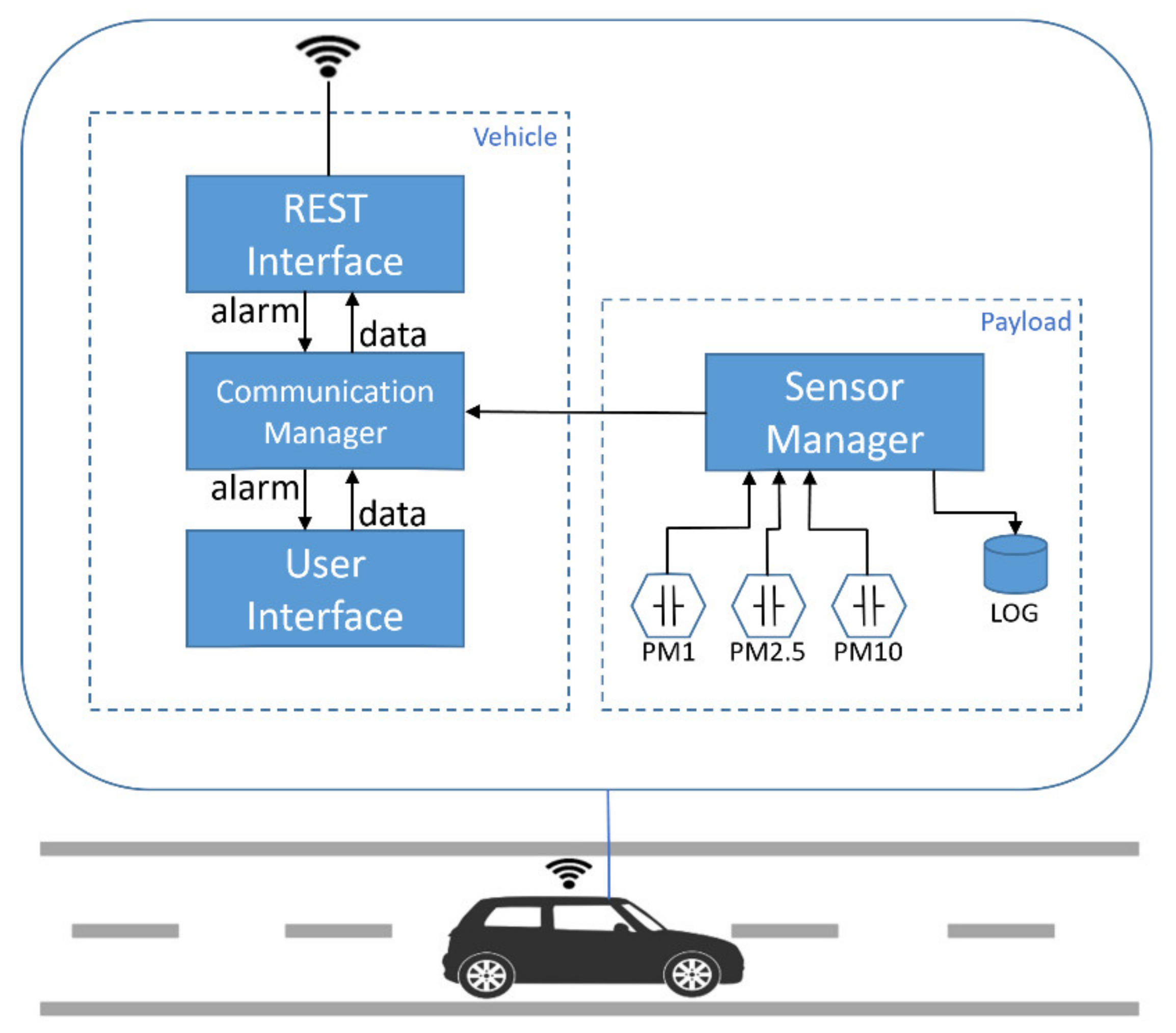
In recent years, miniaturization, other technological advances, and cost reductions have brought to market a number of low-cost sensors designed to measure atmospheric gases and particulate matter. This abundance has fostered the adoption of LCSs by both public authorities and citizen science initiatives [14]. Although LCSs cannot replace traditional reference methods, these sensors have created new opportunities to broaden access to ambient air quality monitoring for applications such as personal health and sub-regional air quality assessment, e.g., to gather neighbourhood-level data to illustrate air quality issues affecting local communities. In addition, the use of standard reference methods implies the use of skilled operators for maintenance and calibration, while LCSs, which do not need skilled personal, open the possibility for broader use [15,16].
Even if the availability of LCSs has dramatically increased, research on the use of this wealth of data in terms of processing, visualisation, and interpretation is still ongoing. Moreover, the characterisation of these sensors with respect to changing environmental conditions is still a subject of study and the research related to sensor aging is still a very open subject [17].
Accuracy and reliability have become unifying research topics. Several papers have been published that tested different LCSs and compared their performances [18]. Protocols have been developed for such testing by different research institutes in the absence of an internationally accepted standardized one.
There are clear indications that the accuracy of LCSs may be low when compared with reference measurements. The main source of inaccuracy is linked to the low selectivity of gas sensors that may measure currents of electrons produced by different redox reactions from different gas species (cross-sensitivity). Moreover, the calibration is performed in some given reference conditions that may introduce biases when used in sensibly different air composition or meteorological conditions. Regarding the particulate matter sensors, these measure light scattering, which is affected by the particle density and hygroscopicity [19].
A further issue is that of aging. Electrochemical sensors, which measure chemical concentrations, usually have a lifetime expectancy as low as 12 to 18 months, but there is very limited research available on their irreversible degradation behaviour. The particulate matter sensors use a physical method, light scattering, to compute concentrations; this allows for a longer lifespan of the sensor and for a possible reset to near factory conditions with a little cleaning.
In this study, in order to demonstrate the proposed monitoring system, an optical particulate matter sensor was used: the Alphasense OPC-N2, which has been evaluated and discussed in [20]. The reasons for such a choice are the above-mentioned longer lifespan of the sensor, its features, and the observation that the particulate content is one of the basic measures used by municipal administrations to make decisions on traffic restrictions or blocks.
The particulate matter sensors are sensitive to high ambient relative humidity (RH > 85%), and in [20] the following correction was introduced:
C = 1 + k 1.65 1 + 1 a w   and   P M c o r r e c t e d = P M m e a s u r e d C
where a w is RH/100 and k is a parameter that describes the degree of hygroscopicity of a particle, which is dependent on the particle’s composition and is around 0.3 ÷ 0.4.
The monitoring system used in this work is shown in Figure 1 (left panel). It is capable of detecting several chemical compounds, particulates (in the three sizes of PM-1, PM-2.5, and PM-10), and some atmospheric physical parameters such as temperature, humidity, and pressure. At the same time, it is equipped with a GPS sensor, thus yielding georeferenced values. A single-board Raspberry Pi computer takes care of the interrogation of the sensors and provides the data to the end user via a Wi-Fi Internet connection by implementing a web service that can be remotely accessed or may autonomously broadcast data. The size of the device is about 10 × 17 × 9 cm, with a weight of around 500 g. It needs a power source in the range of 7–36 V and about 3 W of power. The device was mounted on the laboratory van through the cable hole on the roof of the vehicle (see Figure 1, right panel) in order to model the actual data collection by several devices on board different vehicles.

2.2. The Smart Road

The Smart Road (SR) is a rather fuzzy concept that has been in the limelight in recent years following the smart wave; we are accustomed to the concepts of Smart Cities, Smart Districts, Smart Buildings, and Smart Homes. They all describe the idea of pervasive computing; in other words, all the parts of modern life can be made smart with the help of some processing power, communication capabilities, and, above all, data. The trigger (and at the same time effect) of this smart wave is the so-called Internet of Things (IoT), i.e., the possibility of equipping nearly every electronic device with communication and elaborative powers, together with ever-decreasing costs of computing power and storage memory.
A given road can be made smart in several different respects and, while this idea has been instantiated and implemented in diverse ways in different places, it is intimately linked to the Intelligent Transportation System (ITS) framework [21]. The suggestion is that transport and mobility must be reconsidered as an integrated and, above all, dynamic system where control, information, and management operate synergistically and synchronously [22].
For example, in Sweden the SR is considered as a form of infrastructure able to recharge electric vehicles while they are moving on it [23,24]. In Italy, the main road administrator, ANAS, is currently making some sections of the Italian road network smart with an approach centred on the safety of the journey. They are equipping roadside streetlights with sensors and with a wireless network to communicate with cars and passengers for traffic-related warnings and to monitor the road status [25].
The authors are currently involved in a project to set up an experimental SR in order to study applications and solutions for a better quality of life and energy saving [26]. Through a wireless communication network housed in the roadside lamps, the end users (vehicles, bicyclists, and pedestrians) are able to carry on a dialogue with the Smart City computing centre. This exchange conveys relevant data for different services and applications. As an example, a vehicle may obtain real-time information that it cannot directly and locally access, e.g., an alarm condition on the planned path to be followed or a meteorological alert of some kind. Furthermore, the vehicle can receive instructions concerning its recharging, e.g., where and when, compatible with the overall status of the electrical grid and the wishes of the vehicle itself, such as being near to the trip’s destination. The SR is thus a communication link between the city’s central authority and the single end user that can also be used in the reverse, centripetal way. Any end user may furnish data obtained with proprioceptive sensors (e.g., position, speed, battery charge) or exteroceptive sensors (e.g., air temperature, pollution, road surface conditions) acting as a mobile sensor device and increasing the detail of the description of the current state of the city. In Figure 2 is shown the case in which a vehicle provides data concerning particulate matter.
In the Casaccia Research Centre (Rome), a SR is under construction. It runs for about 700 m and is composed of 22 streetlights. Each pole is equipped with a remotely controlled dimmable LED lamp and may also be equipped with one of the following fixed sensors: a noise sensor, a CO2 sensor, or a particulate matter sensor and a camera that can autonomously control the illumination level through a TAI/FAI approach (TAI, Traffic Adaptive Installation, which controls the illumination on the basis of the traffic intensity; FAI, Full Adaptive Installation, which also adds illumination control on the basis of weather conditions).
On the foot of the street poles runs a fibre link and three access points (APs) are interfaced with it: one at the beginning of the road, one in the middle of the road, and one at the other end of the road. On the Smart Road, an experimental electric vehicle circulates that carries several sensors for the description of the urban environment. For the sake of the present paper, it carries the air monitoring payload described at the end of Section 2.1.
In this work, the LCS represents the IoT device relaying its data to the city’s central processing facility for integrating the data collected from official fixed systems for a higher degree of detail in the monitoring of air pollutants. The idea is that some vehicles in the town are equipped with a mobile air pollutant monitoring system. This system checks the particulate content at a given frequency and then automatically transmits the data back to the city’s central facility. The prototype system is small and light and can conceivably be mounted on almost any vehicle; however, in operational conditions, it may mostly be mounted on board mass transit buses or other service vehicles of the municipality. Thus, the city gathers data from the different mobile systems and interpolates the data both spatially and temporally, greatly increasing the real-time awareness of the pollution situation in the town.
The chosen LCS is the Alphasense OPC-N2, which was mounted on the air monitoring payload and measured the atmospheric particulate content. Through the payload’s Raspberry Pi, the following data can be retrieved: geographical coordinates, time, temperature, barometric pressure, humidity, PM1, PM2.5, PM10, and some internal data (the OPC-N2 bin counts). The total load is circa 300 bytes with an acquisition frequency of 0.5 Hz, i.e., once every two seconds; thus, the data throughput is very low. In the fully deployed SR, the Wi-Fi link may be thought of as being continuous; at present, the payload is able to buffer data locally and transmit them whenever a Wi-Fi AP becomes available. Since the Casaccia Smart Road is not yet complete, the described experimental campaign was carried out in an urban area to demonstrate the feasibility of the conceived approach. During the experimental campaign, the data were stored on board the device and downloaded only at the end.

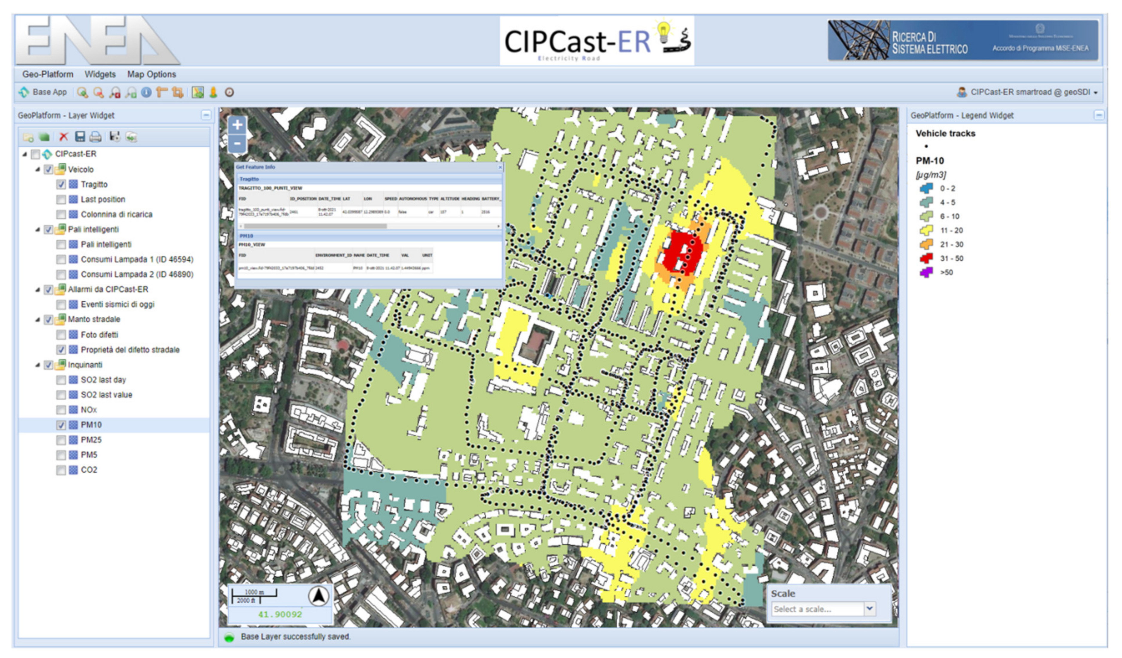
2.3. The CIPCast Platform

The CIPCast platform is a GIS-based DSS conceived and developed by ENEA to support the monitoring, risk analysis, and management of urban infrastructures [7]. It includes and manages more than 400 geospatial data layers for spatial analysis, the protection of infrastructures, and increasing urban assets’ resilience. Moreover, CIPCast implements algorithms and procedures for multicriteria decision processes in order to support interactive monitoring, urban planning, and decision-making [27,28,29,30,31].
CIPCast interacts with the SR infrastructure to perform risk analysis due to extreme natural events, malfunctions, or alerts detected by means of distributed sensors or sensors located in situ. In the latter case, it can receive and integrate data from vehicles, such as spatialised and processed location, status, and air quality data, to provide maps and generate alarms.
All the above-described functions are accessible through the CIPCast interactive geographical interface, a WebGIS application that represents the graphical front-end [31] of the data and information provided and/or produced.
Figure 3 shows a diagram of the software architecture of CIPCast, which can be represented according to the Model View Controller (MVC) paradigm:
-
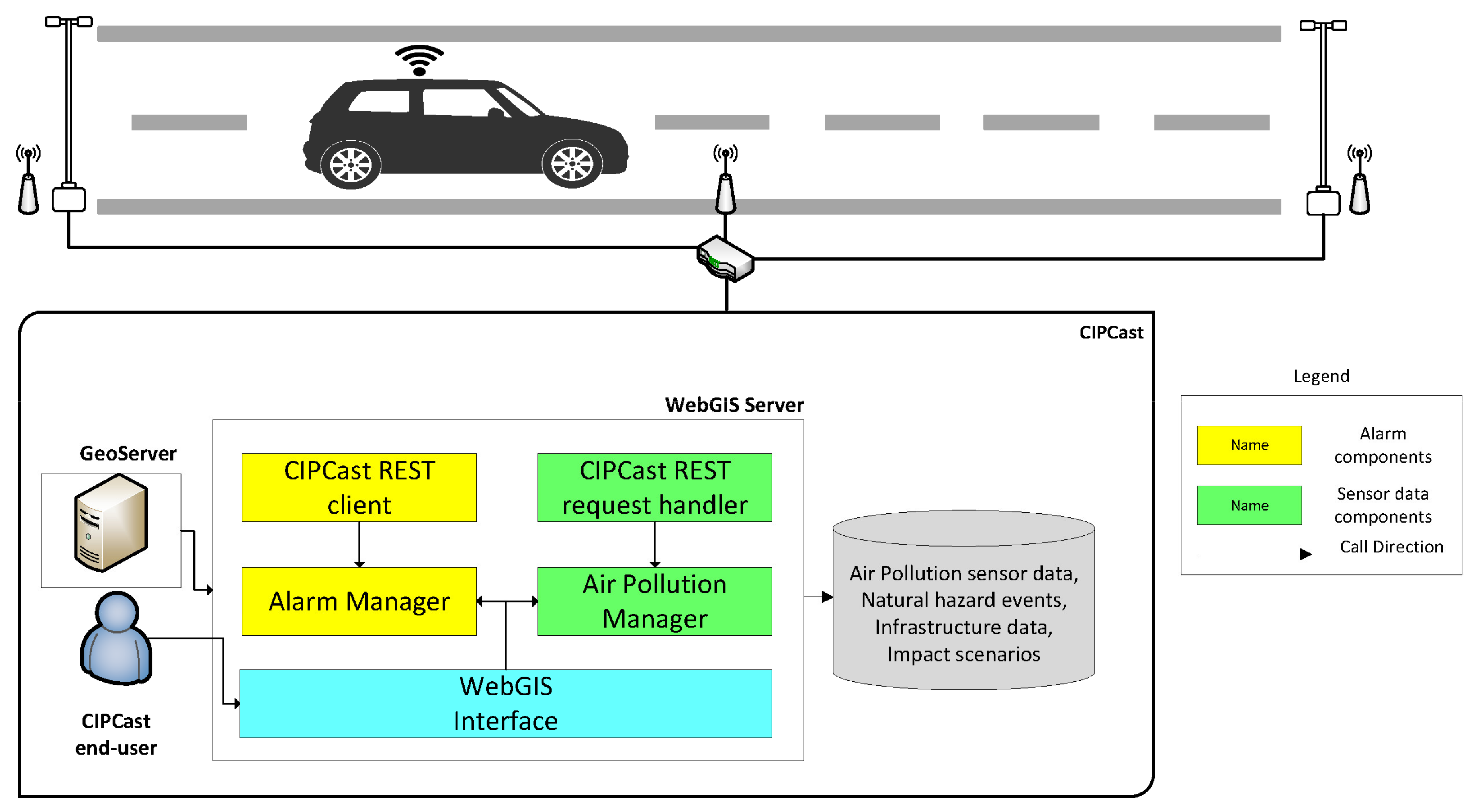
Model: this includes the database that stores the field data acquired from the different sensors and the risk analysis results. Such data are characterised by the time of acquisition, the sensor, and the concentration;
-
View: this provides the Graphical User Interface (GUI) that can support the final end-user by providing her/him the set of GIS layers (e.g., field data, impact scenarios) and the real-time sequence of events in a timeline window; and
-
Controller: this represents the software components that are responsible for acquiring sensor data from the vehicle and for raising alarms when pollution concentration thresholds are exceeded. The communication between CIPCast and the vehicle is performed through the use of REST web services. In particular, the REST Request handler and the REST client represent components responsible for the acquisition of sensor data and for sending alarms to the vehicle, respectively.
In order to manage and process the data collected by the LCS, CIPCast interacts with specific elements of the Smart Road (SR), represented by the roadside lamps. The vehicles circulating in the SR connect to the network through access points installed on some lamps and therefore can communicate data from the LCS directly to CIPCast via TCP/IP protocols using JSON messages carrying the relevant information. Appendix A shows an example of such a message.

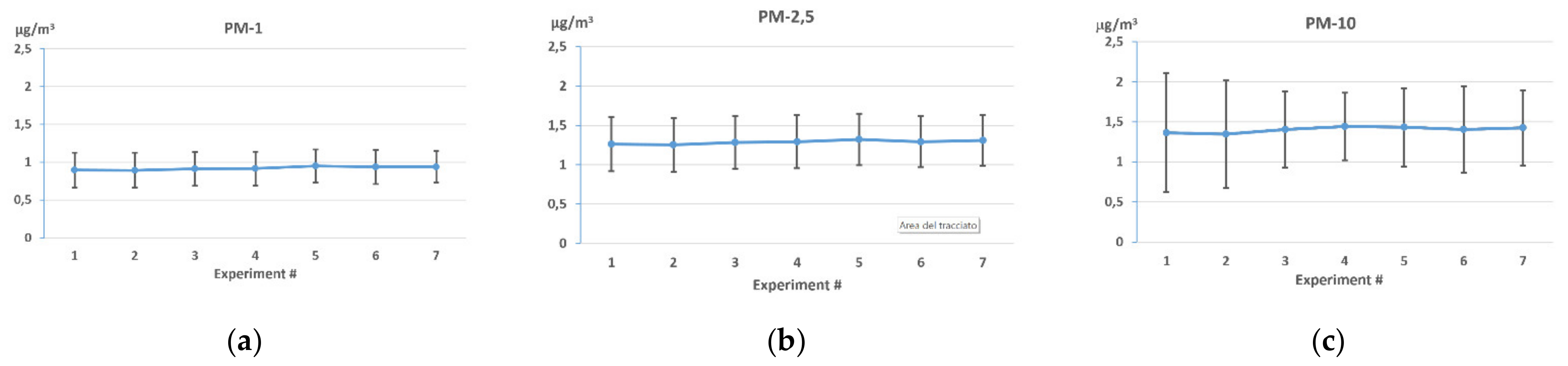
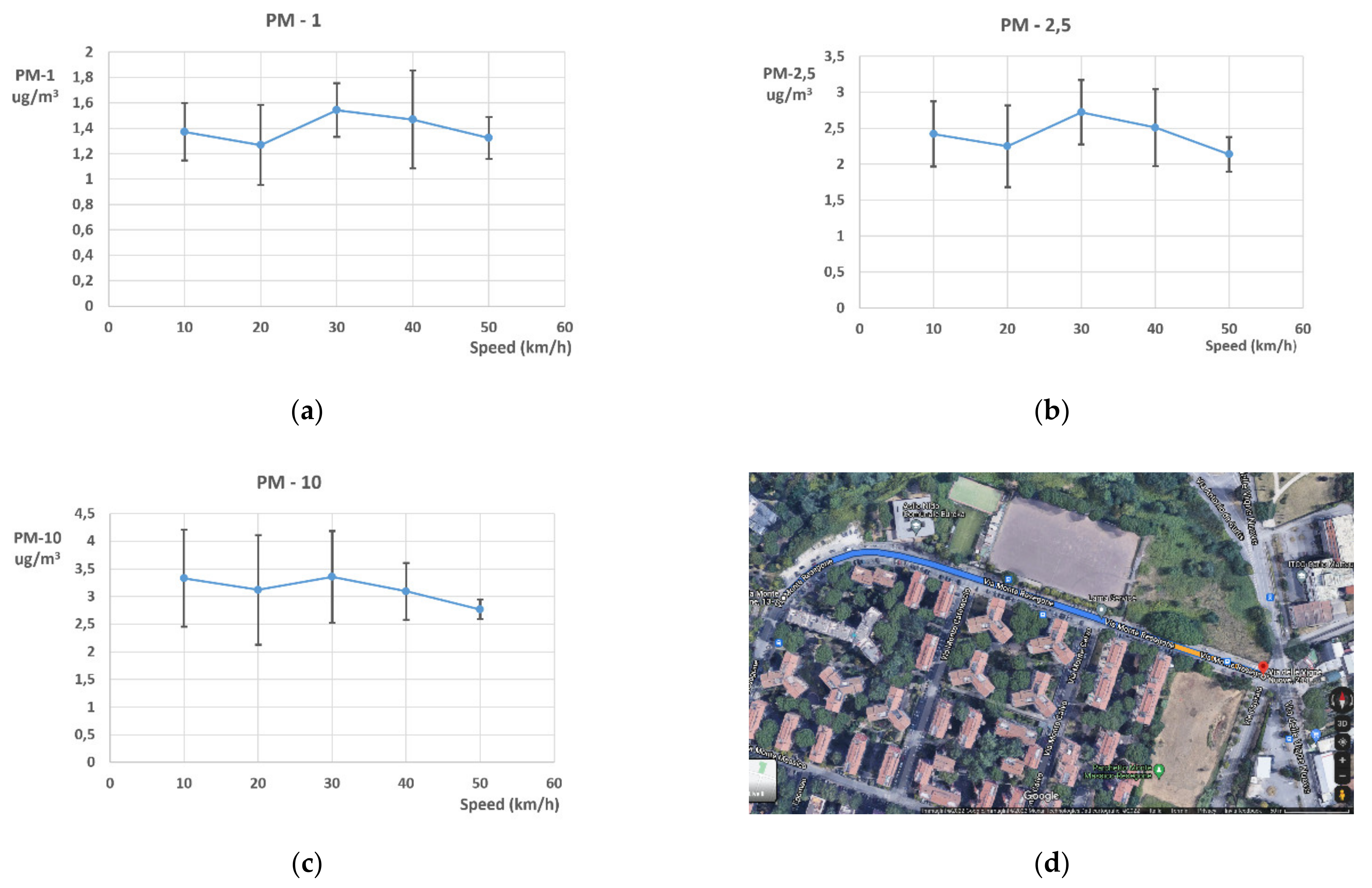
2.4. Preliminary Experimental Data Processing: Sensor Characterisation

Some preliminary measurements were performed before the actual experimental campaign. In detail, an assessment of the stability of measures was carried out. The PM LCS was placed in a closed room with no ventilation and a series of measures were collected. This was done in order to make the sensor measure a stable signal, with no changes due to ventilation, which greatly influences the particulate content. In each experiment, the system measured the particulate content on average for 15 min, with a single datum once every two seconds. The average values with the standard deviation for the seven experiments performed are reported in Figure 4 for the three particulate species PM-1, PM-2.5, and PM-10. Two observations can be made. In each plot, the standard deviations are very similar and the measure is fundamentally the same on a time span of about two hours, showing the stability of measurements of the device. If the coefficient of variance, i.e., the ratio between the standard deviation and the mean value, is computed, the values obtained are 0.24 ± 0.01, 0.26 ± 0.01, and 0.34 ± 0.02, respectively for PM-1, PM-2.5, and PM-10. These values are in good agreement with those in [20], where several Alphasense OPC-N2 sensors are compared.
Once we were in the geographical area where the campaign was conducted and once we had mounted the LCS onto the van, before the actual experimentation, we performed a set of measurements in order to check the variability in the signal with respect to the velocity of the vehicle. The LCS employed possesses a small fan, which ensures a more or less constant flow of air in the sensor. Since the LCS was mounted on board a moving vehicle, it would be interesting to determine whether the air flux caused by the vehicle’s motion would affect the measurements and to what degree.
In order to check this, the van was driven on a low-traffic street, repeating the trajectory, i.e., the same side of the street and the same direction, but at different speeds as indicated by the vehicle’s instrumentation. The considered velocities were 10, 20, 30, 40, and 50 km/h. Among all the recorded PM data, only those recorded at the correct speed were retained, i.e., the acceleration and deceleration phases were discarded. Figure 5 shows the average and standard deviation of the measured data as a function of speed for the three PM values. The measures are very similar, pointing to a substantial degree of independence from the vehicle speed. For PM-10, above 30 km/h the standard deviation decreases, indicating better stability at higher velocities, possibly linked to the more stable air fluxes around the van. It is important to stress that the used street was peripheral and had almost no traffic, under the assumption that the PM content was largely constant; nonetheless, some variability in the PM content there could always exist across the different experimental series, being that the measurements were taken at different times. The measurements were performed in a time window of less than 5 min in order to limit as much as possible the variation in the measured quantity.

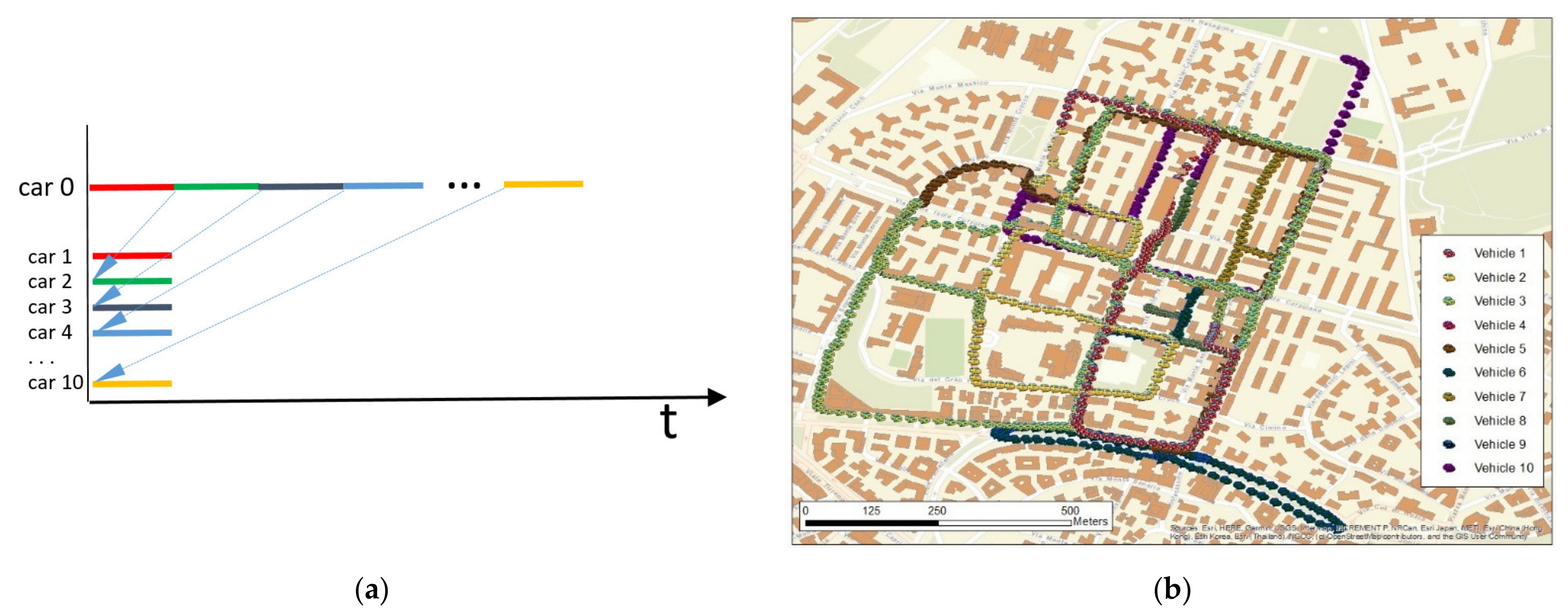
2.5. Experimental Campaign

Some experimental data collection was performed by mounting the system on the roof of a vehicle and driving it through Rome in the neighbourhood of one of the fixed air pollution analysers deployed by the municipality. Several routes that crisscross the area were recorded. The data are particulate concentrations and GPS coordinates, recorded every two seconds on the vehicle’s route. The various paths are plotted in Figure 6b.
The data were recorded via the on-board software by polling all the sensors, saved on the on-board mass memory (an SD card), and downloaded at the end via a Wi-Fi REST interrogation of the system.
The recorded data were rearranged in order to simulate the contemporary recording of data as collected by several different vehicles, each equipped with a sensor, as shown by the coloured dots in Figure 6. The number of simulated vehicles is 10. In order to remove some outliers in the measured data, a threshold was placed at 80 μg/m3 and a centred moving average, of sample window 5, was used to reduce noise. The data were also corrected in accordance with Equation (1) even if the relative humidity while collecting data was low.
In Table 1, the relevant data for the 10 simulated vehicles are presented. The data recording was made with the vehicle moving at an average speed of 17.3 km/h with a minimum of 10.8 km/h and a maximum of 20.6 km/h. The relative sample density was on average 99.6 samples per km with a minimum of 86.7 samples per km and a maximum of 128.6 samples per km, depending on the speed. The total travel length was about 14.1 km, in 48:38, and with 1398 samples recorded that add up to 584 kB of data, as shown in the rightmost column.
As mentioned above, one of the problems related to LCSs is aging. The particulate matter sensors are less prone to this issue as compared with chemical ones. The aging of the sensor can be correlated to a decrease in the reliability of the measure; thus, a simple law was devised to describe this decrease with time from the latest sensor calibration. It is assumed that the sensor’s trustworthiness is a linear function of time:
R e l = R e l 0 k t ,   with   R e l > 0
where R e l 0 is the reliability of the sensor when calibrated, k is an experimental constant to be evaluated, and t is the time since the last calibration. For the sake of demonstration of the idea, different ages were assigned to the different simulated sensors, ranging from 1 (for a new or a newly calibrated sensor) to 5 years, with a decrease in reliability with k = 0.05 and t measured in years. In other words, each simulated sensor measured on the route the concentrations of particulate matter, relaying them to the GIS-based DSS for further processing together with the time of the sensor’s last calibration.

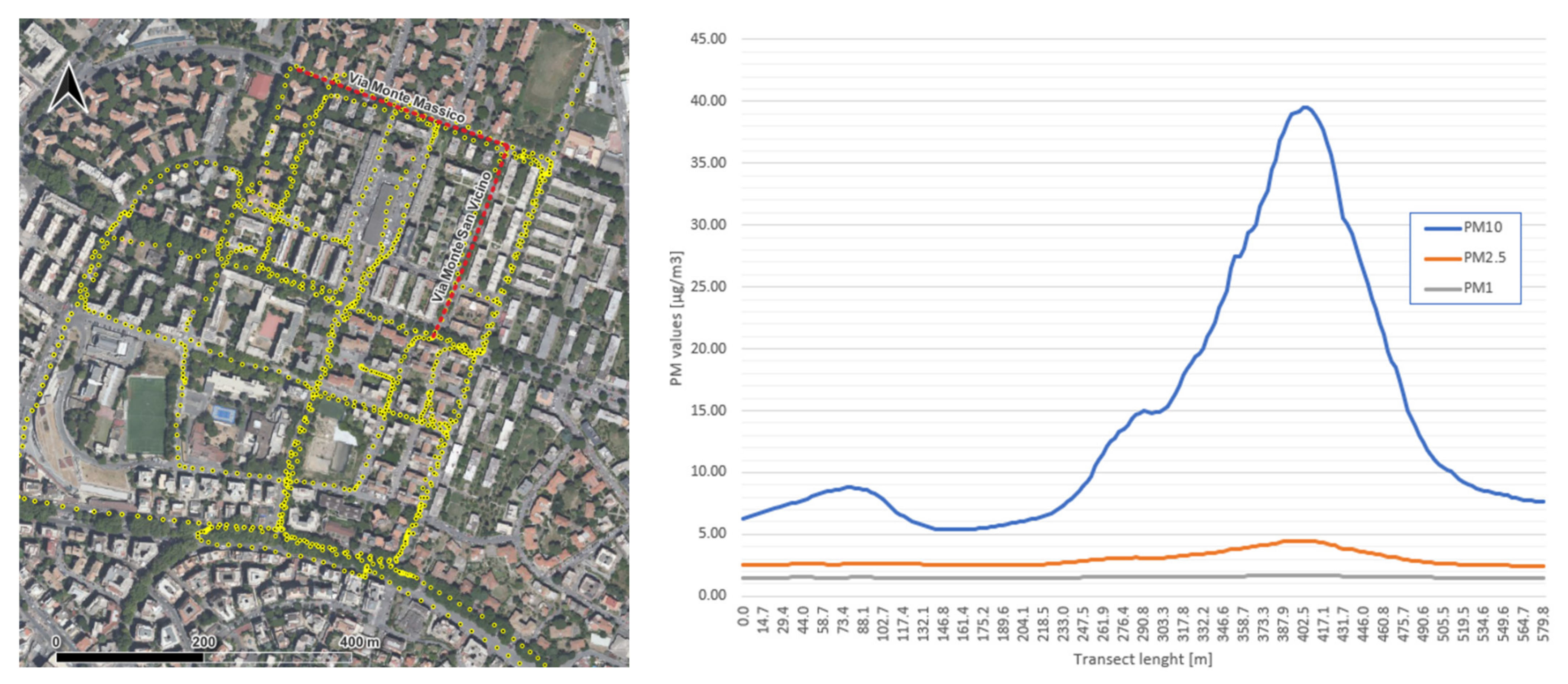
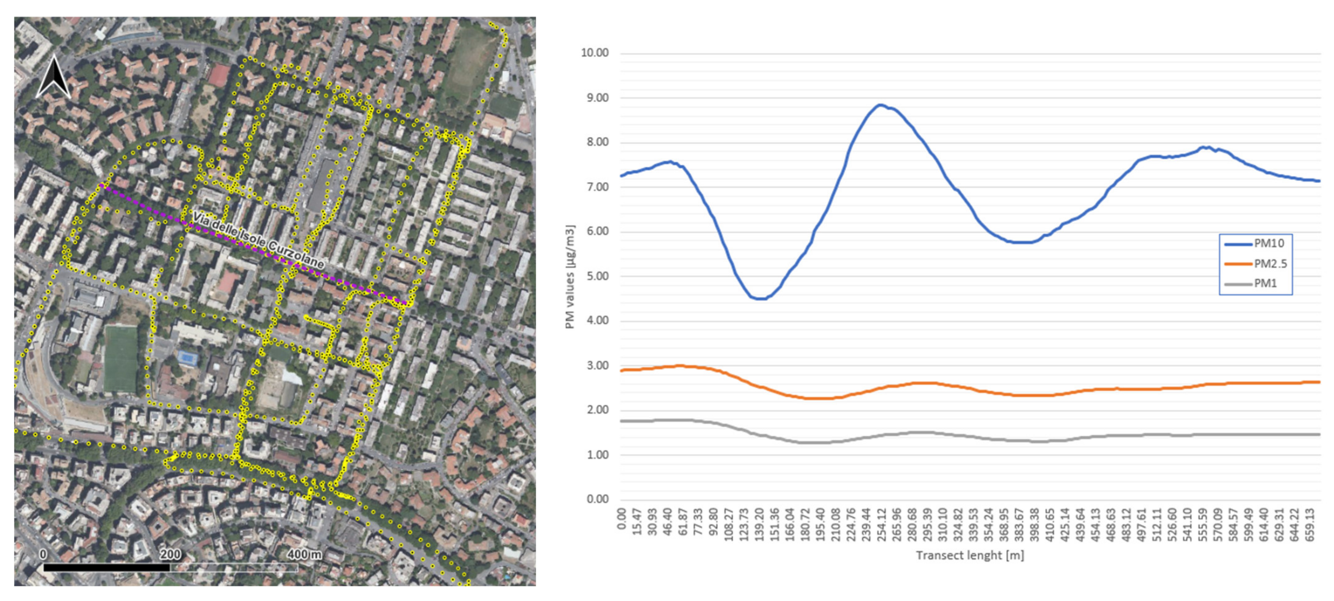
2.6. GIS-Based Data Processing
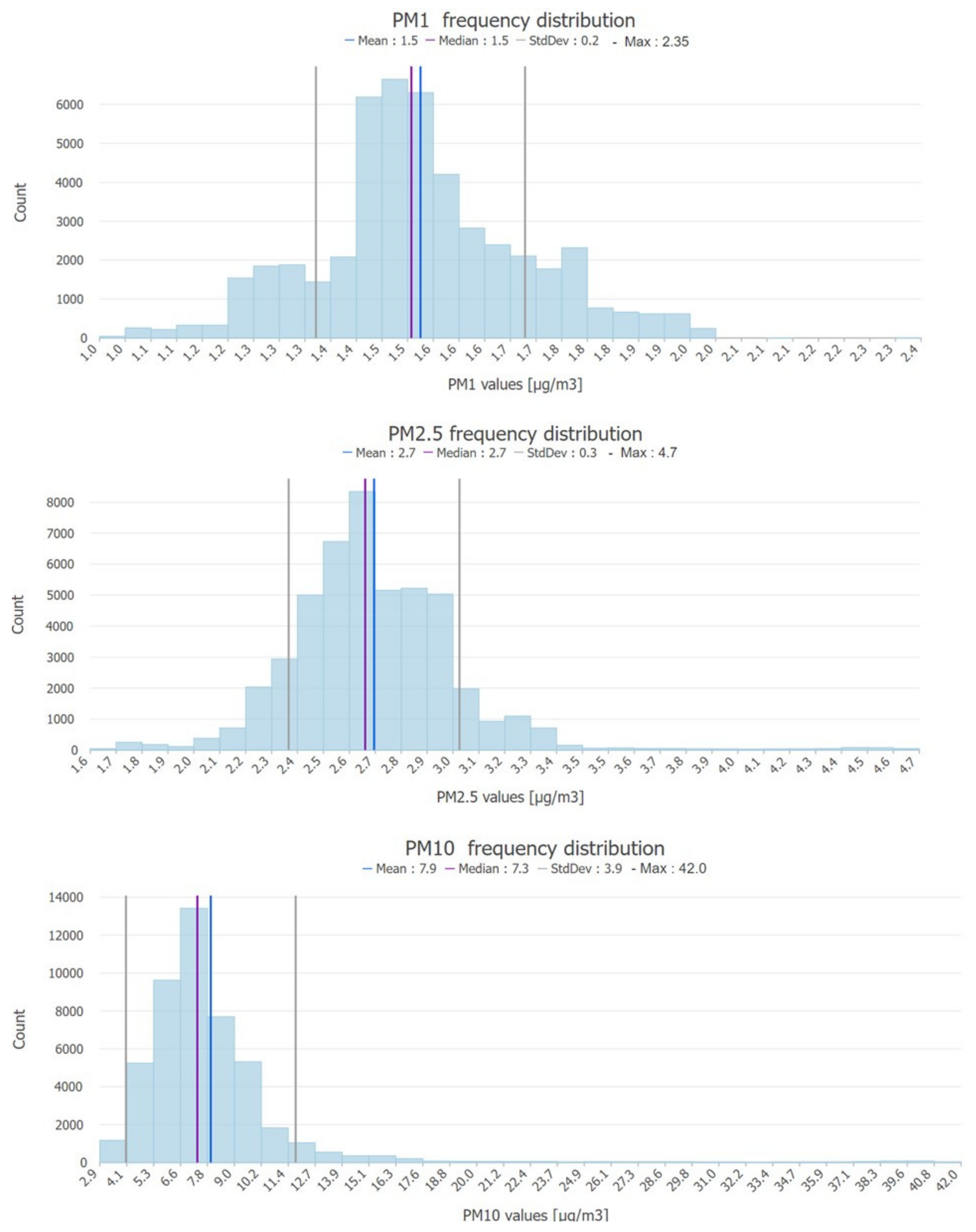
The GIS-based approach used in the present case study to process the measured air quality parameters allows for the spatial assessment and delimitation of areas with similar characteristics (concentration levels, statistical properties of the measured data, etc.) [12]. In addition to the assessment of the spatial representativeness of air pollutant measurements, GIS-based processing can provide tools to model their concentration [32].
The pollutant data (e.g., PM-1, PM-2.5, and PM-10) measured by the LCS installed on board the vehicle and sent to CIPCast consists of a series of georeferenced points along with their characteristics. Once those data are acquired by CIPCast, they are transformed into a standard GIS format. Hence, the WebGIS application is able to manage them, allowing us to query and display the information acquired at each point, which is shown in a pop-up window containing all the descriptive attributes available (timestamp, sensor characteristics, latitude and longitude, pollutant concentration, temperature, etc.).
Subsequently, CIPCast processes the point data transmitted by the sensors in order to produce interpolated maps of particulate concentrations. Numerous interpolation methods are available: a comprehensive overview and discussion are presented in [33] and [34]. Nevertheless, the most commonly used methods (the inverse distance weighting method, the ordinary kriging method, and the spline method), which have been proven to provide reliable and spatially continuous results, are usually implemented in the main GIS software suites. In the present case study, the data were considered using the above-mentioned reliability index (Equation (2)), i.e., a weighted interpolation of the data on the basis of the sensor’s age. Considering the spatio-temporal distribution of the sensors and the characteristics of the monitored area, data were processed using diffusion interpolation with barriers provided by the ESRI ArcGIS suite [35]. Diffusion interpolation refers to the fundamental solution of the heat equation, which describes how heat or particles diffuse with time in a homogeneous medium. Such a prediction is able to gently flow around barriers such as the buildings in the present case. Concerning the surface characteristics, the possible mitigating role of urban green areas was not considered, since the surveys were carried out in a densely built-up neighbourhood.
The data gathered from the vehicles are considered in a time window of 10 min. This means that all the data concur with the interpolation with their own time-from-last-calibration characteristics inside the 10-min window. Any data collected after this time window will be analysed and will be part of the next time window. Thus, the time evolution of the air quality is evaluated six times per hour.

3. Results

The main result of the present work is represented by the definition of a multi-faceted methodology for the assessment of the air quality in an urban context. We have presented a system composed of a lightweight device equipped with a LCS for the measurement of particulate matter, an urban infrastructure for the relay of data among end users, either vehicles or humans, a central facility (a Smart Road), and a GIS-based Decision Support System (the CIPCast-ER platform) able to process real-time data with the aim of possibly issuing local area alarms concerning the air quality.

Particulate Matter Mapping

Data about PM surveys acquired from sensors and sent to CIPCast are processed in the GIS environment as described in the previous section. Then, the PM interpolated maps are produced, as depicted in Figure 7, and stored as GIS layers in the CIPCast geospatial database. In Figure 7, the white polygonal areas correspond to the buildings that were considered to be barriers during the interpolation process. Here, it is possible to observe that in the upper right part of the map for PM-10 there is an anomalous situation, which is also confirmed in the PM-2.5 map.
To this end, it is possible to draw a line on the visualised map and define a transect from which we can obtain the PM values in the interpolated map and then represent them in a graph. As an example, in the present case two transects were sketched. In Figure 8 and Figure 9 are reported the graphs with the different PM trends along each defined transect.
Finally, considering the distribution of PM values in the mapped layers, the application can compute basic statistics such as those reported in Figure 10.
It is important to stress that these data are real time or near real time, allowing for a more accurate study of the pollutants and the possibility of issuing health-related alarms to the local population.
The experimental campaign presented here is relative to a single time window of 10 min, but it can be repeatedly performed to follow the time evolution of the particulate content since the SR would be continuously relaying data to the CIPCast platform and allowing for six pollution status assessments per hour.
For the sake of comparison, the available official ARPA data from the local fixed monitoring station report an average value over the entire day of 18 µg/m3 for the PM-10 content only. The here-reported data, besides also analysing the PM-1 and PM-2.5 content, are relative to a time window of 10 min around 11:00 AM and for the PM-10 content give an average value of about 12 µg/m3 near the ARPA station.

4. Discussion

The central idea presented in this article concerns the availability of a much larger dataset than what would usually be available, gathered with lightweight and small mobile monitoring systems. This, together with the possibility of exploiting a GIS-based DSS for the processing of data in near real time, yields the possibility of monitoring the air quality in an urban area in a more detailed and continuous way.
In many applications, the availability of a large quantity of data, even if they are of a lower quality, yields a non-trivial contribution to the description of a state. The concept of data fusion in many different applications is an example of this approach; to estimate a measurement, several different sensors of different characteristics and precisions can be exploited, all contributing in different degrees to the final value [36,37].
The results here reported show the viability of such an approach to the gathering of neighbourhood-level data in almost real time, allowing for a higher data resolution.
Currently, the data are binned in a given time window (typically 10 min) and the typical duration of the processing is in the order of 10 s. In other words, all the measurements from the different vehicles in this time window are considered to be simultaneous and, consequently, are jointly processed.
Several studies [38,39,40] have measured urban pollution with mobile platforms with the same basic components: a vehicle, some sensors, a GPS unit, and battery power, and collected data on pre-defined routes for a limited period of time. In [41,42], the units were mounted on municipality service vehicles and used to collect large quantities of data each day (see also [43]).
With respect to previous related works (see [4] and references therein), the system here presented, being composed of sensing, communication, and processing parts, has the following strengths.
It considers the direct connection of the sensors to the central elaborative power through a Smart Road, allowing for continuous and timely monitoring of the overall situation in near real time. It currently works by processing data in time windows, assessing the situation several times per hour with geographically denser data, and yielding more precise and timely monitoring results.
One of the components of the system is a DSS (Figure 11) that may issue alarms related to the infringement of pollutant limits. At the same time, the DSS allows us to store data, build historical time-series, and make them available to the end user for further off-line processing or other possible elaborations of pollution data that could be performed on a local neighbourhood scale (e.g., optimal positioning of fixed measurement stations).

5. Conclusions

A system for the monitoring of the particulate content in an urban environment was presented. This system has three main components: a device based on the Alphasense OPC-N2 sensor mounted on board vehicles moving in the area; a Smart Road acting as the link between the city on one side and the vehicles on the other; and a Decision Support System based on a GIS able to elaborate on the data in near real time for the sake of helping the city’s administrators.
We conducted an experimental field campaign to collect data in real time from a neighbourhood in the city of Rome and simulate the contemporary circulation of ten different vehicles with differently aged sensors.
The data load is limited (see Table 1); thus, it is suitable for the Smart Road infrastructure in particular and to any kind of wireless network in general.
The collected data are processed and made available to a GIS, which is conceived of as a DSS for the territory’s managers. The system provides a user-friendly display of maps in given layers of the GIS (similarly to [9,10]), local spatial analysis along given routes of particular importance, and the possibility of setting alarm thresholds.
In this sense, it is possible to consider the whole platform as providing near-real-time monitoring that allows an end user to monitor the atmospheric particulate content in a denser way both in space and in time, opening the way to the possibility of issuing traffic blocks in a more targeted and timely way.
A further research issue involves the processing of measurements in time in order to assess whether the aforementioned time window can be made smaller or to slide in time instead of being a time step.
At present, the system has no memory, i.e., the output of the processing of the current time window does not depend on the previous ones. Further work will aim to determine whether the implementation of memorization capabilities in the platform may provide better results. Another important issue refers to the refining of the data fusion algorithm. For better results, the existing coarse weighted average method will be compared to more refined approaches, such as Kalman filtering or neural networks.

Author Contributions

Conceptualization, Sergio Taraglio and Maurizio Pollino; methodology, Maurizio Pollino and Sergio Taraglio; software, Stefano Chiesa and Antonio Di Pietro; data curation, Stefano Chiesa and Sergio Taraglio; writing—original draft preparation, Sergio Taraglio; writing—review and editing, Sergio Taraglio and Maurizio Pollino; visualization, Maurizio Pollino; supervision, Sergio Taraglio and Maurizio Pollino. All authors have read and agreed to the published version of the manuscript.

Funding

This work was partially funded by the Italian Ministry of Ecologic Transition in the framework of the Triennial Plan 2019–2021 of the Research on the National Electrical System (Piano Triennale 2019–2021 della Ricerca di sistema elettrico nazionale).

Informed Consent Statement

Not applicable.

Acknowledgments

The authors are indebted to Federico Karagulian for discussions on low-cost sensors and their current characteristics and limitations for air pollution measurements. The authors acknowledge the support of Luigi La Porta in addressing WebGIS-related issues and programming. The authors wish to thank the anonymous Referees for their extremely detailed and valuable comments that helped to improve the clarity of the manuscript.

Conflicts of Interest

The authors declare no conflict of interest.

Appendix A

Figure A1 shows an example of a JSON message produced by a vehicle. It consists of four sections:
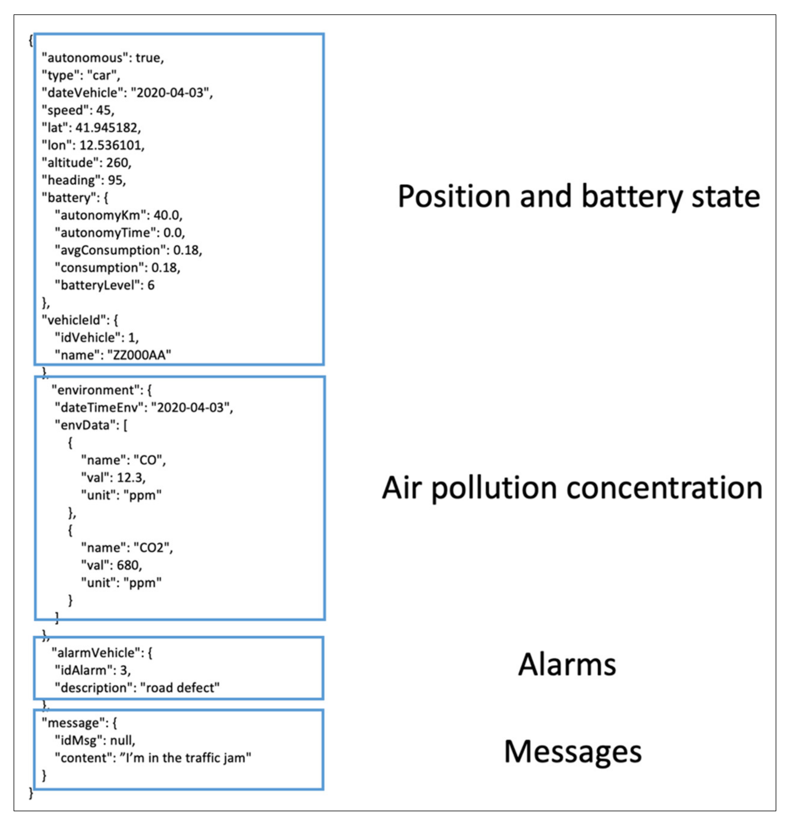
  • Section 1: this section contains general information on the vehicle: the vehicle identifier, latitude, longitude, altitude (m), speed (Km/h), date of acquisition, and autonomous mode;
  • Section 2: this section contains the pollutant concentration values acquired by the sensors;
  • Section 3: this section contains the alarms that can be raised by the vehicle; and
  • Section 4: this section contains possible messages that can be sent autonomously by the vehicle or by the vehicle’s driver.
Figure A1. Example of a JSON message produced by the vehicle and acquired by CIPCast.
Ijgi 11 00132 g0a1

References

  1. Raaschou-Nielsen, O.; Andersen, Z.J.; Beelen, R.; Samoli, E.; Stafoggia, M.; Weinmayr, G.; Hoffmann, B.; Fischer, P.; Nieuwenhuijsen, M.J.; Brunekreef, B.; et al. Air pollution and lung cancer incidence in 17 European cohorts: Prospective analyses from the European Study of Cohorts for Air Pollution Effects (ESCAPE). Lancet Oncol. 2013, 14, 813–822. [Google Scholar] [CrossRef]
  2. European Commission. Material for Clean Air; European Commission: Brussels, Belgium, 2017. [Google Scholar]
  3. ARPA Lazio (Agenzia Regionale per la Protezione Ambientale della Regione Lazio). Available online: https://www.arpalazio.it/ (accessed on 25 September 2021).
  4. Xie, X.; Semanjski, I.; Gautama, S.; Tsiligianni, E.; Deligiannis, N.; Rajan, R.T.; Pasveer, F.; Philips, W. A Review of Urban Air Pollution Monitoring and Exposure Assessment Methods. ISPRS Int. J. Geo-Inf. 2017, 6, 389. [Google Scholar] [CrossRef] [Green Version]
  5. Minet, L.; Liu, R.; Valois, M.-F.; Xu, J.; Weichenthal, S.; Hatzopoulou, M. Development and Comparison of Air Pollution Exposure Surfaces Derived from On-Road Mobile Monitoring and Short-Term Stationary Sidewalk Measurements. Environ. Sci. Technol. 2018, 52, 3512–3519. [Google Scholar] [CrossRef] [PubMed]
  6. Chiesa, S.; Pollino, M.; Taraglio, S. A Mobile Small Sized Device for Air Pollutants Monitoring Connected to the Smart Road: Preliminary Results. In Computational Science and Its Applications—ICCSA 2020; Lecture Notes in Computer Science; Gervasi, O., Murgante, B., Misra, S., Garau, C., Blečić, I., Taniar, D., Apduhan, B.O., Rocha, A.M., Tarantino, E., Torre, C.M., et al., Eds.; Springer: Cham, Switzerland, 2020; Volume 12253, pp. 517–525. [Google Scholar] [CrossRef]
  7. Taraglio, S.; Chiesa, S.; La Porta, L.; Pollino, M.; Verdecchia, M.; Tomassetti, B.; Colaiuda, V.; Lombardi, A. Decision Support System for smart urban management: Resilience against natural phenomena and aerial environmental assessment. Int. J. Sustain. Energy Plan. Manag. 2019, 24, 135–146. [Google Scholar] [CrossRef]
  8. Rhyne, T.; MacEachren, A.M.; Gahegan, M.; Pike, W.; Brewer, I.; Cai, G.; Lengerich, E.; Hardisty, F. Geovisualization for knowledge construction and decision support. IEEE Comput. Graph. Appl. 2004, 24, 13–17. [Google Scholar] [CrossRef] [Green Version]
  9. Balla, D.; Zichar, M.; Tóth, R.; Kiss, E.; Karancsi, G.; Mester, T. Geovisualization Techniques of Spatial Environmental Data Using Different Visualization Tools. Appl. Sci. 2020, 10, 6701. [Google Scholar] [CrossRef]
  10. Pasquaré Mariotto, F.; Antoniou, V.; Drymoni, K.; Bonali, F.L.; Nomikou, P.; Fallati, L.; Karatzaferis, O.; Vlasopoulos, O. Virtual Geosite Communication through a WebGIS Platform: A Case Study from Santorini Island (Greece). Appl. Sci. 2021, 11, 5466. [Google Scholar] [CrossRef]
  11. Banerjee, P.; Ghose, M.K.; Pradhan, K. AHP-based Spatial Air Quality Impact Assessment Model of vehicular traffic change due to highway broadening in Sikkim Himalaya. Ann. GIS. 2018, 24, 287–302. [Google Scholar] [CrossRef] [Green Version]
  12. Righini, G.; Cappelletti, A.; Ciucci, A.; Cremona, G.; Piersanti, A.; Vitali, L.; Ciancarella, L. GIS based assessment of the spatial representativeness of air quality monitoring stations using pollutant emissions data. Atmos. Environ. 2014, 97, 121–129. [Google Scholar] [CrossRef]
  13. Chmielewski, S. Towards Managing Visual Pollution: A 3D Isovist and Voxel Approach to Advertisement Billboard Visual Impact Assessment. ISPRS Int. J. Geo-Inf. 2021, 10, 656. [Google Scholar] [CrossRef]
  14. Kumar, P.; Morawska, L.; Martani, C.; Biskos, G.; Neophytou, M.; Di Sabatino, S.; Bell, M.; Norford, L.; Britter, R. The rise of low-cost sensing for managing air pollution in cities. Environ. Int. 2015, 75, 199–205. [Google Scholar] [CrossRef] [PubMed] [Green Version]
  15. Castell, N.; Dauge, F.R.; Schneider, P.; Vogt, M.; Lerner, U.; Fishbain, B.; Broday, D.; Bartonova, A. Can commercial low-cost sensor platforms contribute to air quality monitoring and exposure estimates? Environ. Int. 2017, 99, 293–302. [Google Scholar] [CrossRef]
  16. Schneider, P.; Castell, N.; Vogt, M.; Dauge, F.R.; Lahoz, W.A.; Bartonova, A. Mapping urban air quality in near real-time using observations from low-cost sensors and model information. Environ. Int. 2017, 106, 234–247. [Google Scholar] [CrossRef] [PubMed]
  17. Clements, A.L.; Griswold, W.G.; RS, A.; Johnston, J.E.; Herting, M.M.; Thorson, J.; Collier-Oxandale, A.; Hannigan, M. Low-Cost Air Quality Monitoring Tools: From Research to Practice (A Workshop Summary). Sensors 2017, 17, 2478. [Google Scholar] [CrossRef] [PubMed] [Green Version]
  18. Karagulian, F.; Barbiere, M.; Kotsev, A.; Spinelle, L.; Gerboles, M.; Lagler, F.; Redon, N.; Crunaire, S.; Borowiak, A. Review of the Performance of Low-Cost Sensors for Air Quality Monitoring. Atmosphere 2019, 10, 506. [Google Scholar] [CrossRef] [Green Version]
  19. Di Antonio, A.; Popoola, O.A.M.; Ouyang, B.; Saffell, J.; Jones, R.L. Developing a Relative Humidity Correction for Low-Cost Sensors Measuring Ambient Particulate Matter. Sensors 2018, 18, 2790. [Google Scholar] [CrossRef] [PubMed] [Green Version]
  20. Crilley, L.R.; Shaw, M.; Pound, R.; Kramer, L.J.; Price, R.; Young, S.; Lewis, A.C.; Pope, F.D. Evaluation of a low-cost optical particle counter (Alphasense OPC-N2) for ambient air monitoring. Atmos. Meas. Tech. 2018, 11, 709–720. [Google Scholar] [CrossRef] [Green Version]
  21. Giannopoulos, G.A.; Mitsakis, E.; Salanova, J.M. Overview of Intelligent Transport Systems (ITS) Developments in and across Transport Modes; JRC Scientific and Policy Reports; Publications Office of the European Union: Luxembourg, Germany, 2012. [Google Scholar] [CrossRef]
  22. Directive 2010/40/EU of the European Parliament and of the Council of 7 July 2010. Available online: https://eur-lex.europa.eu/legal-content/EN/TXT/?uri=CELEX%3A02010L0040-20180109 (accessed on 25 September 2021).
  23. Smart Road “eRoadArlanda”. Available online: https://eroadarlanda.se/ (accessed on 25 September 2021).
  24. Smart Road “Gotland”. Available online: https://www.smartroadgotland.com/ (accessed on 25 September 2021).
  25. ANAS S.p.A. Direzione Operation e Coordinamento Territoriale Infrastruttura Tecnologica e Impianti. In SMART ROAD “La Strada All’avanguardia che Corre Con Il Progresso”; ANAS: Rome, Italy, 2018. (In Italian) [Google Scholar]
  26. Taraglio, S.; Chiesa, S.; Nanni, V.; Pieroni, F.; Pollino, M.; Di Pietro, A.; Montorselli, S.; Bellocchio, E.; Costante, G.; Fravolini, M.L.; et al. The Smart Road Project in ENEA. In Proceedings of the I-RIM 2020 Second Italian Conference on Robotics and Intelligent Machines, Online, 10–13 December 2020; pp. 272–273. [Google Scholar] [CrossRef]
  27. Giovinazzi, S.; Pollino, M.; Kongar, I.; Rossetto, T.; Caiaffa, E.; Pietro, A.D.; Porta, L.L.; Rosato, V.; Tofani, A. Towards a Decision Support Tool for Assessing, Managing and Mitigating Seismic Risk of Electric Power Networks. In Computational Science and Its Applications—ICCSA 2017; Lecture Notes in Computer Science; Gervasi, O., Murgante, B., Misra, S., Garau, C., Blečić, I., Taniar, D., Apduhan, B.O., Rocha, A.M., Tarantino, E., Torre, C.M., et al., Eds.; Springer: Cham, Switzerland, 2017; Volume 10406. [Google Scholar] [CrossRef]
  28. Pollino, M.; Di Pietro, A.; La Porta, L.; Fattoruso, G.; Giovinazzi, S.; Longobardi, A. Seismic Risk Simulations of a Water Distribution Network in Southern Italy. In Computational Science and Its Applications—ICCSA 2021; Lecture Notes in Computer Science; Gervasi, O., Murgante, B., Misra, S., Garau, C., Blečić, I., Taniar, D., Apduhan, B.O., Rocha, A.M., Tarantino, E., Torre, C.M., et al., Eds.; Springer: Cham, Switzerland, 2021; Volume 12951. [Google Scholar] [CrossRef]
  29. Modica, G.; Pollino, M.; La Porta, L.; Di Fazio, S. Proposal of a Web-Based Multi-criteria Spatial Decision Support System (MC-SDSS) for Agriculture. In Innovative Biosystems Engineering for Sustainable Agriculture, Forestry and Food Production; MID-TERM AIIA 2019; Lecture Notes in Civil Engineering; Coppola, A., Di Renzo, G., Altieri, G., D’Antonio, P., Eds.; Springer: Cham, Switzerland, 2020; Volume 67. [Google Scholar] [CrossRef]
  30. Coletti, A.; De Nicola, A.; Di Pietro, A.; La Porta, L.; Pollino, M.; Rosato, V.; Vicoli, G.; Villani, M.L. A comprehensive system for semantic spatiotemporal assessment of risk in urban areas. J. Contingencies Crisis Manag. 2020, 28, 178–193. [Google Scholar] [CrossRef]
  31. Di Pietro, A.; Lavalle, L.; La Porta, L.; Pollino, M.; Tofani, A.; Rosato, V. Design of DSS for Supporting Preparedness to and Management of Anomalous Situations in Complex Scenarios. In Managing the Complexity of Critical Infrastructures; Studies in Systems, Decision and Control; Setola, R., Rosato, V., Kyriakides, E., Rome, E., Eds.; Springer: Cham, Switzerland, 2016; Volume 90. [Google Scholar] [CrossRef] [Green Version]
  32. Vicente, A.B.; Juan, P.; Meseguer, S.; Serra, L.; Trilles, S. Air Quality Trend of PM10. Statistical Models for Assessing the Air Quality Impact of Environmental Policies. Sustainability 2019, 11, 5857. [Google Scholar] [CrossRef] [Green Version]
  33. Li, J.; Heap, A.D. A review of comparative studies of spatial interpolation methods in environmental sciences: Performance and impact factors. Ecol. Inform. 2011, 6, 228–241. [Google Scholar] [CrossRef]
  34. Lepot, M.; Aubin, J.-B.; Clemens, F.H.L.R. Interpolation in Time Series: An Introductive Overview of Existing Methods, Their Performance Criteria and Uncertainty Assessment. Water 2017, 9, 796. [Google Scholar] [CrossRef] [Green Version]
  35. ESRI ArcGIS. Available online: https://www.esri.com/en-us/arcgis/about-arcgis/overview (accessed on 25 September 2021).
  36. Durrant-Whyte, H. Multi Sensor Data Fusion; Australian Centre for Field Robotics, The University of Sydney: Sydney, NSW, Australia, 2001. [Google Scholar]
  37. Bertino, L.; Evensen, G.; Wackernagel, H.H. Sequential data assimilation techniques in oceanography. Int. Stat. Rev. 2003, 71, 223–241. [Google Scholar] [CrossRef]
  38. Wallace, J.; Corr, D.; Deluca, P.; Kanaroglou, P.; McCarry, B. Mobile monitoring of air pollution in cities: The case of Hamilton, Ontario, Canada. J. Environ. Monit. 2009, 11, 998–1003. [Google Scholar] [CrossRef]
  39. Wang, M.; Zhu, T.; Zheng, J.; Zhang, R.; Zhang, S.; Xie, X.; Han, Y.; Li, Y. Use of a mobile laboratory to evaluate changes in on-road air pollutants during the Beijing 2008 Summer Olympics. Atmos. Chem. Phys. 2009, 9, 8247–8263. [Google Scholar] [CrossRef] [Green Version]
  40. Shi, Y.; Lau, K.K.L.; Ng, E. Developing street-level PM2.5 and PM10 land use regression models in high-density Hong Kong with urban morphological factors. Environ. Sci. Technol. 2016, 50, 8178–8187. [Google Scholar] [CrossRef] [PubMed]
  41. Shirai, Y.; Kishino, Y.; Naya, F.; Yanagisawa, Y. Toward On-Demand Urban Air QualityMonitoring using Public Vehicles. In Proceedings of the 2nd International Workshop on Smart, Trento, Italy, 12–16 December 2016; ACM: New York, NY, USA, 2016; p. 1. [Google Scholar] [CrossRef]
  42. Gao, Y.; Dong, W.; Guo, K.; Liu, X.; Chen, Y.; Liu, X.; Bu, J.; Chen, C. Mosaic: A low-cost mobile sensing system for urban air quality monitoring. In Proceedings of the IEEE INFOCOM 2016—The 35th Annual IEEE International Conference on Computer Communications, San Francisco, CA, USA, 10–14 April 2016; IEEE: Piscataway, NJ, USA, 2016; pp. 1–9. [Google Scholar] [CrossRef]
  43. Hasenfratz, D.; Saukh, O.; Walser, C.; Hueglin, C.; Fierz, M.; Thiele, L. Pushing the spatio-temporal resolution limit of urban air pollution maps. In Proceedings of the 2014 IEEE International Conference on Pervasive Computing and Communications (PerCom), Budapest, Hungary, 24–28 March 2014; IEEE: Piscataway, NJ, USA, 2014; pp. 69–77. [Google Scholar] [CrossRef]
Figure 1. Air monitoring payload and its location on the roof of the van.
Ijgi 11 00132 g001
Figure 2. The Smart Road: a vehicle may carry on a dialogue with the city by exchanging data and alarm conditions.
Ijgi 11 00132 g002
Figure 3. CIPCast–ER software architecture diagram.
Ijgi 11 00132 g003
Figure 4. Stability measures in seven experiments (the error bars are standard deviations): (a) PM-1; (b) PM-2.5; (c) PM-10.
Ijgi 11 00132 g004
Figure 5. PM sensor measurements as a function of velocity (the error bars are standard deviations): (a) PM-1; (b) PM-2.5; (c) PM-10; (d) the trajectory along which the data were collected.
Ijgi 11 00132 g005
Figure 6. The experimental campaign: (a) the rearrangement of the data from a single recording to several smaller recordings; (b) the resulting location of data points on the map.
Ijgi 11 00132 g006
Figure 7. The results of the interpolation with barriers: (a) PM-1; (b) PM-2.5; (c) PM-10.
Ijgi 11 00132 g007
Figure 8. PM-1 (gray), PM-2.5 (orange), and PM-10 (blue) trends along transect 1 (Via Monte Massico–Via Monte S. Vicino, depicted in red on the map. PM acquisitions are depicted in yellow).
Ijgi 11 00132 g008
Figure 9. PM-1 (gray), PM-2.5 (orange), and PM-10 (blue) trends along transect 2 (Via delle isole Curzolane, depicted in violet on the map. PM acquisitions are depicted in yellow).
Ijgi 11 00132 g009
Figure 10. Frequency distribution of interpolated PM-1, PM-2.5, and PM-10 values in the area of interest.
Ijgi 11 00132 g010
Figure 11. The CIPCast DSS: an example of a visualisation of the PM-10 map within the WebGIS interface.
Ijgi 11 00132 g011
Table 1. Characteristics of the simulated vehicles’ trips.
Trip IDSample CountDuration (mm:ss)Distance (m)Samples/kmSpeed (km/h)Size (kB)
11183:57128891.619.643
21264:13136392.419.451
330210:09314096.218.6109
41555:12178886.720.661
51545:111363113.015.856
61645:301546106.116.966
7551:4958194.719.221
8581:5564889.520.322
91294:201003128.613.947
101374:42141397.018.0108
Publisher’s Note: MDPI stays neutral with regard to jurisdictional claims in published maps and institutional affiliations.

