Abstract
Averaging GPS trajectories is needed in applications such as clustering and automatic extraction of road segments. Calculating mean for trajectories and other time series data is non-trivial and shown to be an NP-hard problem. medoid has therefore been widely used as a practical alternative and because of its (assumed) better noise tolerance. In this paper, we study the usefulness of the medoid to solve the averaging problem with ten different trajectory-similarity/-distance measures. Our results show that the accuracy of medoid depends mainly on the sample size. Compared to other averaging methods, the performance deteriorates especially when there are only few samples from which the medoid must be selected. Another weakness is that medoid inherits properties such as the sample frequency of the arbitrarily selected sample. The choice of the trajectory distance function becomes less significant. For practical applications, other averaging methods than medoid seem a better alternative for higher accuracy.
1. Introduction
Averaging time series signals is an open problem for which solutions are needed in many practical applications such as trajectory clustering [1,2] and extraction of road segments from Global Positioning System (GPS) recordings [3,4,5]; see Figure 1 and Figure 2. Average can be defined as the point in the data space that minimizes the squared distance from all data points. However, to find the optimal average for sequences is time consuming because there is an exponential number of candidates for the average. It has been shown to be a computationally difficult (NP-hard) problem in the case of DTW space [6], which would require exponential time to solve optimally.
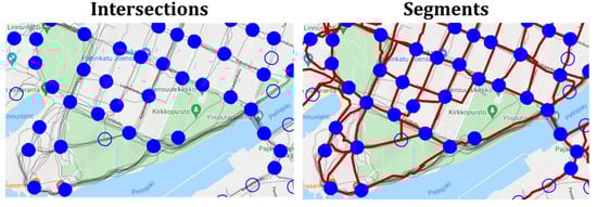
Figure 1.
Extracting road network from GPS trajectories needs segment averaging to convert a set of trajectories between two intersections to a road segment.
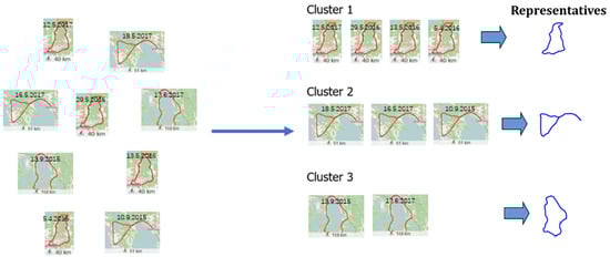
Figure 2.
Averaging is needed to find representatives for trajectory clusters. This can be challenging as the trajectories may have complex shapes.
GPS sequences differ from time series in that the pointwise alignment is performed in 2-d geographical space (latitude, longitude) instead of 1-d time space. Spatial locations of the points form the data and their time stamps are here excluded. If included, the problem would become averaging of sequences in 3-d space. The GPS trajectories can also be very noisy due to GPS errors [7]. Thus, the two main challenges of the averaging problem are that (1) the individual points do not align, and (2) the number of points can vary significantly between the different sequences. Even the simplified 1-d version with fixed-length signal is a computationally difficult, NP-hard problem.
Medoid is a practical alternative for averaging. It has been widely used in many applications in spatial data mining, text categorization, vehicle routing, and clustering just to name few [8,9,10,11]. It is defined as the object in the set for which the average distance to all the objects of the cluster is minimal [12]. It is a similar concept to mean with the difference that mean can be any point in the data space while medoid is restricted to be one of the objects in the set. Medoid is used when mean cannot be easily defined, or when simple averaging can create artificial combinations that do not appear in real life. Medoid has two main benefits compared to mean. First, there are only k candidates to choose from, which makes it computationally solvable. Second, it is expected to be less biased by outliers in the data.
In clustering, medoid has been used to replace the well-known k-means algorithm [13,14] by its more robust variant called k-medoids [15], motivated by the assumption that it is more robust to noise. Similarly to k-means, it first selects clusters representatives at random. Second, the nearest representatives are searched, and each point is partitioned to the cluster with closest representative. A new set of representatives are then calculated as the medoids for each cluster. The process is iterated similarly as in k-means.
K-means itself is only a local fine-tuner and it performs poorly if the number of clusters is high. Using a cleverer initialization method or re-starting the algorithm multiple times can improve the result, but only if the clusters are not completely separated [16]. This can be overcome by a simple wrapper around the k-means, called random swap [17], which swaps the centroids in a trial-and-error manner but manages to find the correct centroid location whenever the data have clusters [18]. A similar extension to k-medoid has also been applied by a method called partitioning around the medoid (PAM) [15].
Another interesting result was found in [19] when comparing performance of k-means and random swap with noisy data. Random swap worked significantly better with the clean data but when the amount of noise increases it removed the superiority of random swap and both algorithms performed equally poorly. In fact, k-means benefitted from the noise because it creates more overlap between the clusters, which helps k-means to move the centroids between the clusters [20]. These findings indicate that noise robustness of any method is all but self-evident and the effect can be something other than what one might expect by common sense.
The difference between mean and medoid is illustrated in Figure 3 with a set of four trajectories. Medoid is one of the input trajectories, which can restrict its usefulness in the case of small sets. In this case, the optimal location of the mean is somewhere in between, but there is no suitable candidate trajectory to choose from; medoid is just the best among the available choices. Medoid is expected to work well if there are sufficient trajectories in the set to choose from. Medoid also has other problems. Since it is one sample from the input set, it will carry all the properties of the selected sample (both good and bad). It does minimize the distance to the other trajectories, but it does not average the other properties such as sample frequency, length, or shape of the trajectories. These might deteriorate its performance in practice.
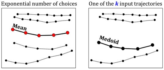
Figure 3.
Examples of using mean (left) and medoid (right) for segment averaging.
Despite the potential benefits of medoid, practical results in [7] were quite discouraging. All studied averaging heuristics performed significantly better than medoid regardless of the distance function. However, medoid was used merely as a reference method and not really considered seriously, while all the heuristics were carefully tuned submissions to the segment-averaging challenge. It is therefore an open question whether medoid is really so poor or whether it could also be tuned for better performance by applying the same pre-processing and outlier-removal tricks that were used within the other methods. To find answers to these questions, we conducted a systematic study of the usefulness of medoid for the averaging problem. Our goal was to answer the following questions:
- What is the accuracy of the medoid?
- When does it work and when not?
- Does it work better than existing averaging techniques in the case of noisy data?
- Which similarity function works best, and how much does the choice matter?
The rest of the paper is organized as follows. The problem is defined in Section 2, describing several alternatives. Medoid is defined in Section 3 and a brief review is given on existing works using medoid. Data sets and the tools used for the experiments are described in Section 4. Main results are then reported in Section 5, followed by more detailed analysis in Section 6. Conclusions drawn in Section 7.
2. Segment Averaging
The averaging task is seemingly simple as calculating average of numbers is trivial, and it is easy to generalize from scalar to vectors in multivariate data analysis. However, averaging time series is significantly more challenging as the sample points do not necessarily align. It is possible to solve the averaging problem by using mean, which is defined as any possible sequence in the data space that minimizes the sum of squared distances to all the input sequences [7]:
Here, X = {x1, x2, …, xk} is the sample input set and C is their mean, which is also called centroid. However, the search space is huge and an exhaustive search by enumeration is not feasible. Some authors consider the problem so challenging that they think it is not self-evident that the mean would even exist [6,21]. However, their reduction theorem showed that mean exists for a set of dynamic time warping (DTW) spaces [6] and the existing heuristics have, therefore, theoretical justification. An exponential time algorithm for solving the exact DTW-mean was recently proposed in [22]. GPS trajectories differ from time series in a few ways. First, the alignment of the time series is performed in the time domain, whereas the GPS points need to be aligned in geographical space. Second, GPS data can be very noisy, which means that mean might not even be the best solution to the averaging problem.
2.1. Heuristics for Finding Segment Mean
Due to the difficulty of finding the optimal mean, several faster but sub-optimal heuristics have been developed. In [13], average segments (called centerline) were used for k-means clustering of the GPS trajectories to detect road lanes. The averaging method was not defined in the paper, but it was later described in [23] as piecewise linear regression. The points are considered as an unordered set and piecewise polynomials are fit with continuity conditions at the knot points [24]. The disadvantage of the regression approach is that the order of the points is lost, and it can make the problem even harder to solve.
The CellNet segment-averaging method [25] selects the shortest path as the initial solution [26], which is iteratively improved by the majorize–minimize algorithm [1]. Trajectory box plot is a similar iterative approach, which divides the trajectories into sub-segments by clustering and, then, at each step, performs piecewise averaging of the sub-segments [27]. Kernelized time elastic averaging (iTEKA) is another iterative algorithm for the averaging problem [28]. It considers all possible alignment paths and integrates a forward and backward alignment principle jointly. There are several reasonable algorithms in literature, although many of them suffer from quadratic time complexity and their implementation can be rather complicated.
The problem was addressed in a recent segment-averaging challenge (http://cs.uef.fi/sipu/segments/, accessed on 24 November 2021) where several heuristic methods were submitted and compared against each other. A new baseline was also constructed by synthesis of the best components of the methods from the competition, as summarized in Figure 4. The first step is to re-order the trajectories to make them invariant to the travel order. Outlier removal is applied in the second step to reduce the effect of noisy trajectories. These steps reduce the problem to a standard sequence averaging problem and the majorize–minimize algorithm [1] is then applied. The last step (optional) is merely to simplify the final representation by the Douglas–Peucker polygonal algorithm [29].
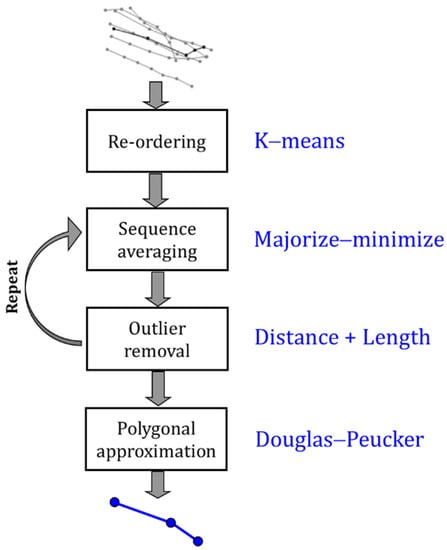
Figure 4.
General structure of the methods from the segment-averaging competition [7]. A new baseline (shown by blue) was constructed by synthesis of these methods.
2.2. Medoid
Median is often used instead of mean because it is less sensitive to noise. In the case of scalar values, median can be easily obtained by first sorting the n data values and then selecting the middle value from the sorted list. However, multivariate data lack natural ordering, which makes it difficult to find the “middle” value. Spatial median [30] constructs the median for each scalar value separately and the result is the concatenation of the independent scalar medians. However, GPS trajectories can have variable lengths and the individual points cannot be trivially aligned to match the points from which the median should be calculated.
It is possible to define median also as a minimization problem so that median is the input point which has minimum average distance to all the other points in the set. A generalization of this to multivariate data is known as medoid. It is defined as the input data object whose total distance to all other observations is minimal. Its main advantage is that the problem then reduces the linear search problem: find the input object that satisfies this minimization objective. Formally, we define medoid as [7]:
where D is a distance or similarity function between two GPS trajectories xi and xj. In other words, medoid is defined as an optimization problem, similar to how we defined mean in Equation (1). The difference is that, instead of allowing any possible trajectory in the space, medoid is restricted to be one of the input trajectories. This reduces the search space significantly, and theoretical time complexity of finding medoid can be as low as O(nk2), where k is the number of trajectories, and n is the number of points in the longest trajectory.
The definition also requires that we have a meaningful distance function between the data objects. This increases the time complexity as calculating distances between trajectories is not trivial. Given k trajectories of n points each, most distance functions take O(n2) time, which makes the time complexity of medoid O(k2n2). However, some of the measures have faster variants such as Fast-DTW [31], which can reduce this to O(k2n).
2.3. Hybrid of Heuristics and Medoid
In [32], a hybrid method was proposed by combining a simple averaging heuristic for linear segments and another method for more complex curves. The linear model uses three descriptors: source (S), median (M), and destination (D). The method first analyzes the complexity of the segment based on the three descriptors to estimate whether the simple linear model can be used, or the more complex alternative should be used. Medoid was used as the alternative method in the variant called RapSeg-B. Figure 5 (left) shows the general structure of the hybrid method.
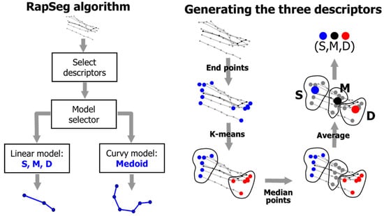
Figure 5.
Overall structure of the RapSeg algorithm [32] and the creation of the three descriptors.
The method creates three separate sets. Endpoints of each trajectory are first collected and clustered by k-means to form two sets: source set and destination set. The travel direction is ignored but the idea itself generalizes even if the directions were preserved. The third set, called median set, is created from the middle points of the trajectories. The centroids are then calculated for each of the three sets to create the three descriptors (S, M, D), as in Figure 5 (right). To decide whether the linear model can be used, a straight-line SD is compared against the three-point polygon SMD which makes a detour via the middle point M. The more the detour deviates from the direct connection, the less likely a simple linear model is suitable to describe this segment. This is measured by cosine of the angle ∠SDM and ∠DSM; if it is smaller than a threshold, then medoid is used.
3. Similarity Measures
Medoid is defined as the trajectory in the set that minimizes the total distance (or maximizes the total similarity) to all other trajectories in the set. For this, we need to choose a distance or similarity measure. Dynamic time warping is probably the most common, but it is sensitive to sub-sampling, noise, and point shifting. It also does not correlate well with human judgement, according to [5]. We will next briefly describe the measures and then perform extensive comparison of the segment averaging using all these measures. The measures and their properties are summarized in Table 1.

Table 1.
Summary of the considered distance measures. The properties are taken from [5], except IRD and HC-SIM, which we added here using our subjective understanding. Human score is the correlation of the measure with human evaluation made in [7]. Most of the measures are also found in the web tool: http://cs.uef.fi/mopsi/routes/similarityApi/demo.php (accessed on 24 November 2021).
3.1. Cell Similarity (C-SIM)
Cell similarity (C-SIM) uses a grid to calculate the similarity. It first creates the cell representation of the trajectories and then counts how many common cells the two trajectories share relative to the total number of unique cells they occupy [5]. An advantage of the method is that it is much less affected by change in sampling rate, point shifting, and noise. A drawback is that the method ignores the travel order, but a recent extension to make it direction-sensitive is proposed in [41].
3.2. Hierarchical Cell Similarity (HC-SIM)
Hierarchical cell similarity (HC-SIM) extends C-SIM to multiple zoom levels. The idea is that small differences can be tolerated if the curves have good match at the higher levels; see Figure 6. C-SIM uses a grid of 25 × 25 m and counts how many cells the segment shares relative to the total number of cells they occupy. HC-SIM uses six zoom levels, with the grid sizes of 25 × 25 m, 50 × 50 m, 100 × 100 m, 200 × 200 m, 400 × 400 m, and 800 × 800 m. In the case of data normalized to the (0,1) scale, the following sizes are used: 0.5%, 1%, 2%, 4%, 8%, 16%. The individual counts are then summed up. Given two trajectories A and B, their hierarchical cell similarity (with L zoom levels) is calculated as follows [7]:
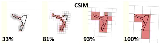
Figure 6.
Hierarchical cell-similarity measure (HC-SIM) is constructed by summing up CSIM-values using different zoom levels. In the example, the two trajectories have only one short detour and minor differences showing only at the densest zoom level. At the highest zoom level, the curves are considered identical.
3.3. Euclidean Distance
Euclidean distance [39] is one of the simplest possible methods. It calculates the distance between the points having the same index. Its main advantages are the simplicity and invariance to the travel order. The only challenge is that the GPS points (latitude and longitude) must be converted into Cartesian coordinates first. The measure is likely to fail when the sampling rates of the two trajectories are very different, or when the two trajectories are otherwise similar but one of them is much longer. The problem is the lack of any alignment of the points, which is addressed in all of the other measures in one way or another.
3.4. Longest Common Subsequence (LCSS)
Longest common subsequence (LCSS) was originally designed for string similarity. The longest common subsequence for strings GETEG, GEGTG, GEGET is GET. The main benefit of LCSS distance between two trajectories is that it allows leaving of far-away (noisy) GPS points as unmatched, with only a minor penalty in the score [42]. Such noise points can have major impact on distance measures that require pair-matching of every point.
3.5. Edit Distance on Real Sequence (EDR)
Edit distance on real sequence (EDR) [35] is derived from the Levenshtein edit distance [43]. It counts how many insert, delete, and replace operations are needed to convert one string to another. For example, when converting bitter to sitting, we first replace “b” to “s” (sitter), then “e” with “i” (sittir), “r” with “n” (sittin), and finally insert “g” and at the end (sitting). The Levenshtein distance is therefore 4. EDR applies edit distance to trajectories by declaring two points identical if they are within the distance ε from each other. In this paper, the value of ε is 0.05. Compared to Euclidean distance, it reduces the effect of noise but both LCSS and EDR are very sensitive to sub-sampling.
3.6. Dynamic Time Warping (DTW)
Dynamic time warping (DTW) [44] is similar to edit distance but instead of exact matching, it calculates the distance between the matched points. It is commonly used to calculate the distance of time series with various lengths and applies straightforwardly to GPS trajectories as well. The drawback of DTW is that it is sensitive to the sampling rate.
3.7. Edit Distance with Real Penalty (ERP)
Edit distance with Real Penalty [37] is a metric variant of EDR that resembles DTW. It calculates the distance between the matched points. However, in the case of a non-match situation, it uses constant 1 rather than using binary value (0/1) as EDR or calculating distance to the neighboring points as DTW. This modification makes the measure metric and allows utilization of triangular inequality property in searches and making efficient indexing structures such as B+ trees.
3.8. Fréchet and Hausdorff Distances
Hausdorff distance [45] is the maximum distance of all nearest points in the two trajectories. It only cares about the longest distance and is therefore sensitive to noise, differences in sampling rate, and point shifting. A single noise point can make the distance very large even if the trajectories would be otherwise a perfect match. Fréchet distance [40] is the same as Hausdorff but the points cannot be matched to those in the past. Fréchet therefore enforces the order of the travel whereas Hausdorff is invariant to it.
3.9. Interpolated Route Distance (IRD)
Interpolation route distance (IRD) [33] is similar to DTW, with two main differences. First, it pairs points from the two trajectories A and B by using interpolation when the other trajectory has fewer samples along some part of the route. This can provide a significantly more accurate distance estimate when the two trajectories have different sampling rates. Second, it has linear time implementation, which makes it significantly faster than the straightforward implementation of DTW taking quadratic time.
4. Experimental Setup
We experiment the averaging with medoid using the data available from the segment-averaging competition [7]; see Table 2. The data consist of segments extracted from four trajectory datasets: Joensuu 2015 [5], Chicago [3], Berlin, and Athens [4]. Joensuu 2015 contains mostly walking, running, and bicycle trajectories collected by Mopsi users. It has high point frequency, 3 s on average, and the data are noisy because of slow movement and low-end smartphones used for the data collection. Chicago contains longer and simpler segments collected by a university shuttle bus. Some segments are noisy due to the tall buildings alongside the route which cause the GPS signal to bounce. The data in Athens and Berlin sets were collected by car with much lower point frequency, 42 s (Berlin) and 61 s (Athens). These segments are simpler, containing only a few points.
Table 2.
Summary of the data used in the experiments. The data were divided into two parts: 100 sets for training (10%) and 901 sets for testing (90%). In total, there are k = 10,480 trajectories with N = 90,231 points. The training data were publicly available in the segment-averaging competition [7], while the testing data were published only afterwards. They are both available here: http://cs.uef.fi/sipu/segments (accessed on 24 November 2021).
All experiments were run using Dell R920 machine with 4 × E7-4860 (total 48 cores), 1 TB, 4 TB SAS HD. The processing time of medoid with all the similarity measures took more than one hour (>1 h) in all cases, while the comparative method (baseline) took only seconds. For this reason, we did not record the exact times, as medoid is clearly slower.
We test the performance of medoid with eleven similarity measures as follows. First, we generate segment averages for each set using medoid with the selected distance measure. The result is compared against ground truth using HC-SIM, which was found to correlate best to human judgment in [7]. The higher the similarity, the better is the result. We also test the effects of two pre-processing techniques: re-ordering of the points and outlier removal. The re-ordering is expected to remove the effect of the travel order and improve measures affected by it. Outlier removal is expected to help when averaging noisy sets.
We use Mopsi web tools (see Figure 7) and the related API in the experimentation: http://cs.uef.fi/sipu/mopsi/ (accessed on 24 November 2021). These include various web pages to demonstrate the operation of a method. Some allow uploading of own data and others provide APIs to be used by those with sufficient programming skills. The following tools, at least, are available:
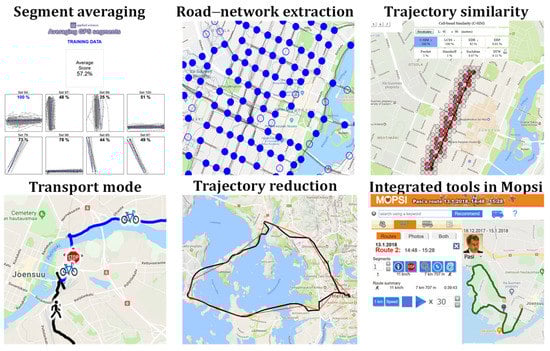
Figure 7.
Summary of the Mopsi web tools available for others to test the segment averaging and related methods.
- Segment averaging [7]http://cs.uef.fi/sipu/segments/training.html (accessed on 24 November 2021)
- Road-network extraction [25]http://cs.uef.fi/mopsi/routes/network (accessed on 24 November 2021)
- Similarity of trajectories [5]http://cs.uef.fi/mopsi/routes/similarityApi/demo.php (accessed on 24 November 2021)
- Transport-mode detection [46]http://cs.uef.fi/mopsi/routes/transportationModeApi (accessed on 24 November 2021)
- Trajectory reduction [47]http://cs.uef.fi/mopsi/routes/reductionApi (accessed on 24 November 2021)
- Tools integrated in Mopsihttp://cs.uef.fi/mopsi/ (accessed on 24 November 2021)
The segment-averaging web page is the most relevant as it allows users to test their own algorithm with the training data by uploading segmentation results in text format. The tool visualizes the uploaded average segments and calculates their HC-SIM scores, but it is limited to 100 training data only. The test data are available, but not via this interactive tool. The road-network extraction tool demonstrates the resulting intersections and segments in between five algorithms. It demonstrates an application where the segment averaging is needed. The trajectory-similarity tool demonstrates the performance of 8 distance measures (lacking only the most recent measures, IRD and HC-SIM) with seven pre-selected datasets. Unfortunately, it does not currently allow testing with users’ own data.
The transport-mode-detection tool allows users to upload their own trajectories and it outputs the detected segments and their predicted stop points and movement types (car, bicycle, run, walk). The trajectory-reduction tool performs polygonal approximation for user-input trajectory with five different quality levels. There are several other tools integrated directly in the Mopsi system without specific interfaces, including C-SIM-based similarity search [5] and gesture-based search where user inputs approximate route by free-hand drawing [48]. In summary, while most results in this paper have been obtained by inhouse implementations, there are APIs and useful web tools available for the reader to perform their own experiments directly related to GPS trajectory processing.
5. Results
The overall results of the training data and test data without pre-processing are summarized in Table 3, sorted from best to worst (training data). Results from the baseline segment averaging are also included from [7]. The three main observations from the results are:
Table 3.
Evaluation of medoid accuracy with various similarity measures on trajectories data with and without pre-processing. Results are given separately for the training and testing data. The corresponding results for the baseline segment averaging [7] are 66.9% (training) and 62.1% (testing).
- HC-SIM performs best with the training data.
- The choice of distance function has only a minor effect.
- The results of medoid are significantly worse than the baseline averaging [7].
The first observation is not surprising. It is expected that optimizing for the same measure that is used in the evaluation will perform best, and it is, therefore, logical to use HC-SIM as the similarity measure with medoid. The second observation, however, is more important. The difference between the best (HC-SIM = 59.9%) and the worst (Euclidean = 56.7%) is only 3.2%-unit for the training data without pre-processing. The difference (55.7% vs. 54.1%) becomes even smaller with the test data (1.7%-unit). Their score distributions are also similar; medoid with LCSS, DTW, EDR, C-SIM, and Euclidean has more poor segments (<30%) than HC-SIM but most segments are still within the 40–70% interval (varying from 434 to 474); see Table 4 and Figure 8. The third observation is the most important: all these results are significantly worse than the baseline averaging result, which is 66.9% for training data and 62.1% for testing data [7]. This demonstrates that the root cause for the performance is medoid itself, not the similarity measure.
Table 4.
Frequency distribution of the scores (901 test datasets) without pre-processing.
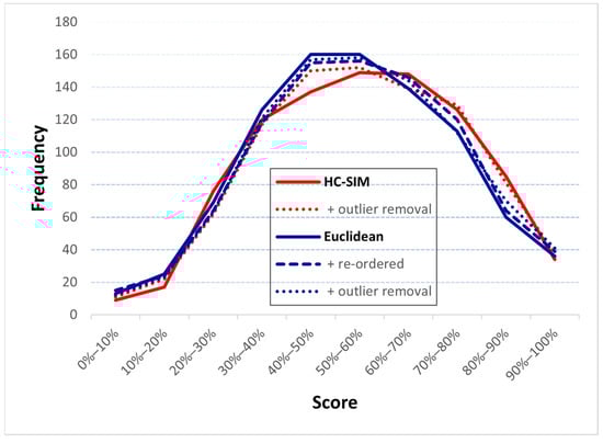
Figure 8.
Frequency histograms of the scores when using HC-SIM (red) and Euclidean (blue).
We also analyze the effect of re-ordering and outlier removal. For these, we use the techniques from the baseline in [7]: k-means for re-ordering, and distance and length criterion for outlier removal. Note that medoid does not necessarily need re-ordering if the distance measure is invariant to the travel order. This is the case with Hausdorff, C-SIM, and HC-SIM. However, the other distance functions are sensitive to the point order: DTW, ERD, ERP, LCSS, Fréchet, and Euclidean. If these are employed, re-ordering might become necessary. However, the results in Table 3 show that, while pre-processing improves the results in most cases, the overall effect remains moderate. Re-ordering slightly improves Fréchet, and Euclidean, especially on a data set whose segment-averaging score falls between 40% and 90% (Table 4). Outlier detections improve the results of EDR, DTW, FastDTW, and LCSS for averaging scores between 70% and 90%. On average, the average performance of medoid improves from 54.8% to 54.9%, but the results are still significantly worse than the baseline segment-averaging method in [7] (62.1%), which shows that these two techniques are not enough to compensate for the weaknesses of medoid.
The IRD result shows that outlier removal does not have a significant effect on many of the GPS data sets. On a few occasions, outlier removal has some positive effects, but not significantly. Re-ordered average scores for C-SIM, HC-SIM and Hausdorff remain the same.
6. Detailed Analysis
We next analyze the effect of various parameters such as noise and set size, and pre-processing techniques including re-ordering, outlier removal, and normalization by resampling.
6.1. Noise
Figure 9 shows a few examples where the chosen medoid has unusual properties that do not describe the data very well. As a reference, the first example (left) is a case where medoid works very well. The distance to ground truth reaches 100% and there is no visible difference between them. This set has plenty of samples and medoid manages to select the trajectory that is also visually pleasing. The other cases, however, demonstrate different problems.
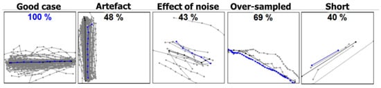
Figure 9.
Examples of sets of k trajectories (gray lines) averaged by medoid with DTW distance (blue line). Black line is the ground truth.
The second example (Artefact) in Figure 9 might be a reasonable choice as it is in the middle of the samples, even if slightly offset from the ground truth. However, the chosen trajectory has an unwanted artefact at the top by having a small peak towards the right. The third example (Noise) shows the effect of noise. While medoid is expected to be more robust to noise than mean, this is not the case in practice. The one far-away sample is enough to pull the medoid from the centre line, decreasing the score to 43%. The fourth example (Over-sampled) has a reasonably good score and is visually close to the ground truth. The problem is that it has an overwhelming number of sample points even if it might have good averaging properties otherwise. The last example (Short) shows the phenomenon where the shortest segment is chosen as the medoid despite it being outermost among all choices.
6.2. Re-Ordering and Outlier Removal
Selected sets are shown in Figure 10 to demonstrate some of the effects of re-ordering and outlier removal. Re-ordering and outlier removal can help occasionally especially when LCSS is used but the effect with HC-SIM seems almost random. The outlier removal failed to detect many obvious outliers. The main reason is that it only analyzes the points but not the entire trajectories. This is a potential future improvement for segment averaging in general, not only with medoid.
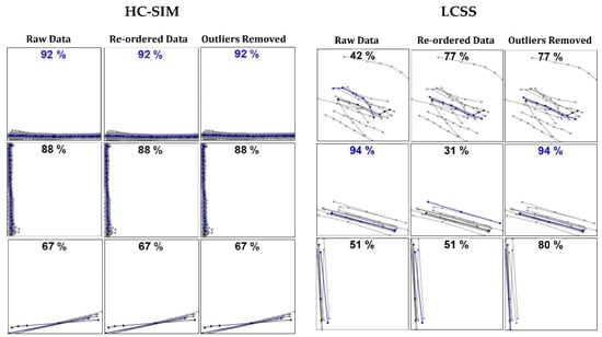
Figure 10.
Selected examples of medoid with HC-SIM and LCSS similarity measures. Blue line is the average result, and black line is the ground truth.
6.3. Normalizing
We next study the effect of normalizing the trajectories by re-sampling before selecting medoid. Figure 11 shows four examples when the input data are first processed so that each trajectory consists of the same number of points (10). We can see that, in all these cases, the result is better both visually and according to the numerical score. The result still copies the artefacts of the selected trajectory but, due to the post-processing, most severe artefacts such as oversampling and zig–zag effect have been eliminated.
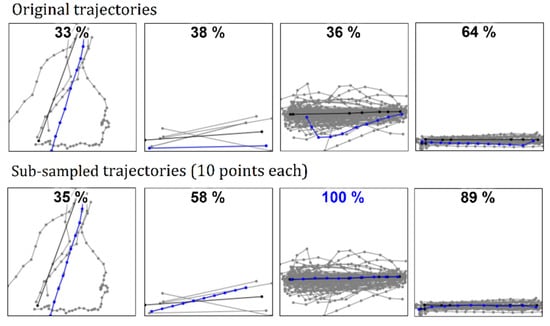
Figure 11.
Pre-processing the trajectories by re-sampling can overcome some issues of medoid. LCSS measure was used in these examples. The re-sampling (to 10 points) is shown only for the segment average (blue line).
6.4. Size of Sets
The main deficiency of medoid originates from the lack of data to choose a good medoid. HC-SIM, IRD, and Hausdorff are the three similarity measures that perform best with training data, while HC-SIM, C-SIM, and IRD perform best with test data, in terms of being closest to the ground truth. However, they also have the fewest segments with a score lower than 40%. Figure 12 shows a few cases when the score is below 30%. We can see that all cases have only a few samples. However, the first case (Set 27) has only three trajectory samples, which are too few to capture the real road segment (black line), which is offset from the samples. The second case (Set 87) has similar offset, but the third example (Set 35) shows tendency of medoid to select the shortest segment despite the fact that the longer segment in the middle would be more sensible. An important observation is that all three methods make the same choices, so the behavior can be attributed mainly to the medoid itself, not to the choice of the distance measure.
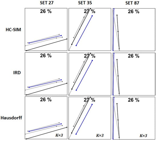
Figure 12.
Examples where medoid provides low score with the three best-performing distance measures. The number of trajectories is very small in all cases: k = 3.
6.5. Number of Points
Results for selected sets with HC-SIM and DTW are plotted in Figure 13 and Figure 14 to demonstrate the effect of the set size and outlier removal. Here, the number with the circle shows the number of trajectories, and x-axis is the logarithmic value of the number of points in the set. The results show that the performance of medoid increases with the data size. The sets with a large number of points have significantly higher scores, and most of the low-scoring sets are those with only few trajectories and points. We observe that the number of trajectories in the set, and the number of points in each trajectory, affect the performance of medoid. The more = points and trajectories there are, the better the score. Outlier removal improves the performance of some of those sets that have few trajectories and points.
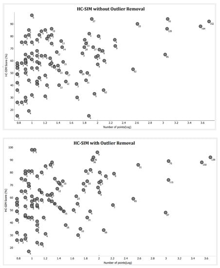
Figure 13.
Result of 100 datasets plotted as a function of the number of points (log scale) in the set. Results are for HC-SIM before outlier removal (above) and HC-SIM after outlier removal (below). Each dot represents one set and the number shows how many trajectories are in the set.
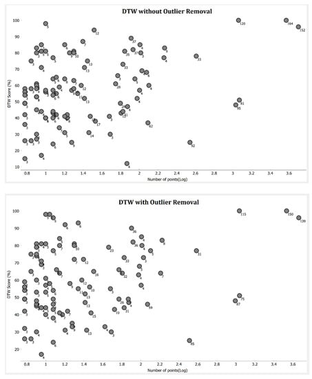
Figure 14.
Result of 100 datasets plotted as a function of the points (log scale) in the set. Results are for DTW before outlier removal (above) and DTW after outlier removal (below). Each dot represents one set and the number shows how many trajectories are in the set.
7. Conclusions
It would be tempting to use medoid for averaging GPS segments because of its simplicity and presumed resistance for outliers. In reality, however, it suffers from several problems that restrict its usefulness in practice. We list here the following weaknesses observed in our experiments:
- Accuracy of medoid is clearly inferior to the best averaging heuristics (baseline).
- Contrary to expectations, medoid is vulnerable to noise.
- Medoid tends to select short segments.
- Medoid copies the (sometimes unwanted) properties of the original trajectory.
- It is slow (averaging of all sets takes >1 h).
Medoid provides quality scores of 59.9% (training) and 54.7% (test) when using the HC-SIM similarity measure without pre-processing of dataset. This is much lower than that of the baseline segment averaging with 66.9% (training) and 62.1% (test). Medoid works poorly especially when there are only few samples to choose from. If the size of the set is large, there are better chances of finding a more accurate representative. Medoid also tends to select short segments. It averages only the overall shape but ignores other features such as segment length and number of sample points. These will be arbitrarily chosen from the original data and the quality of medoid therefore depends a lot on the quality of data.
For these reasons, we do not recommend using medoid, and the existing averaging heuristics seems more promising. Medoid should be avoided especially when the number of samples is low. Some of its deficiencies can be overcome by noise removal and normalizing the input trajectories by re-sampling. These steps are also included in the other averaging heuristics. The other main design question would be the choice between fast sequence averaging, such as the majorize–minimize algorithm, or the time-consuming brute-force algorithm required by medoid. From the efficiency point of view, there is no reason to use medoid; it is fast only when the number of samples is low, but this is also the case when its quality is low.
The effect of similarity measure was of secondary importance. HC-SIM performed best, but the results became very close to each other when the pre-processing techniques were applied. The average scores of the five best-performing measures (C-SIM, HC-SIM, IRD, EDR, LCSS) are only within 0.3%-unit from each other (56.0%, 55.9%, 55.9%, 55.7%, 55.7%). To sum up, the problem of medoid is not the choice of the similarity measure but the general limitation of the medoid itself, as it is restricted to selecting one of the input trajectories as the average. This limitation is likely to appear in other applications where medoid is used.
Author Contributions
Conceptualization, Radu Mariescu-Istodor and Pasi Fränti; methodology, Radu Mariescu-Istodor and Pasi Fränti; software, Radu Mariescu-Istodor; validation, Biliaminu Jimoh; investigation, Biliaminu Jimoh and Pasi Fränti; writing—original draft preparation, Biliaminu Jimoh; writing—review and editing, Pasi Fränti; visualization, Biliaminu Jimoh and Pasi Fränti; supervision, Pasi Fränti. All authors have read and agreed to the published version of the manuscript.
Funding
This research received no external funding.
Institutional Review Board Statement
Not applicable.
Informed Consent Statement
Not applicable.
Data Availability Statement
https://cs.uef.fi/sipu/segments/ (accessed on 24 November 2021).
Conflicts of Interest
The authors declare no conflict of interest.
References
- Hautamäki, V.; Nykanen, P.; Fränti, P. Time-series clustering by approximate prototypes. In Proceedings of the International Conference on Pattern Recognition, Tampa, FL, USA, 8–11 December 2008; pp. 1–4. [Google Scholar]
- Buchin, K.; Driemel, A.; van de L’Isle, N.; Nusser, A. Klcluster: Center-based Clustering of Trajectories. In Proceedings of the 27th ACM SIGSPATIAL International Conference on Advances in Geographic Information Systems (SIGSPATIAL ’19), Chicago, IL, USA, 5–8 November 2019; pp. 496–499. [Google Scholar]
- Biagioni, J.; Eriksson, J. Inferring road maps from global positioning system traces: Survey and comparative evaluation. Transp. Res. Rec. 2012, 2291, 61–71. [Google Scholar] [CrossRef] [Green Version]
- Ahmed, M.; Karagiorgou, S.; Pfoser, D.; Wenk, C. A comparison and evaluation of map construction algorithms using vehicle tracking data. GeoInformatica 2015, 19, 601–632. [Google Scholar] [CrossRef] [Green Version]
- Mariescu-Istodor, R.; Fränti, P. Grid-based method for GPS route analysis for retrieval. ACM Trans. Spat. Algorithms Syst. (TSAS) 2017, 3, 8. [Google Scholar] [CrossRef]
- Jain, B.J.; Schultz, D. Sufficient conditions for the existence of a sample mean of time series under dynamic time warping. Ann. Math. Artif. Intell. 2020, 88, 313–346. [Google Scholar] [CrossRef]
- Fränti, P.; Mariescu-Istodor, R. Averaging GPS segments competition 2019. Pattern Recognit. 2021, 112, 107730. [Google Scholar] [CrossRef]
- Estivill-Castrol, V.; Murray, A.T. Discovering associations in spatial data—An efficient medoid based approach. In Research and Development in Knowledge Discovery and Data Mining; Lecture Notes in Artificial Intelligence; Springer: Berlin/Heidelberg, Germany, 1998; Volume 1394. [Google Scholar]
- Mukherjee, A.; Basu, T. A medoid-based weighting scheme for nearest-neighbor decision rule toward effective text categorization. SN Appl. Sci. 2020, 2, 1–9. [Google Scholar] [CrossRef]
- Fränti, P.; Yang, J. Medoid-Shift for Noise Removal to Improve Clustering. In Proceedings of the International Conference on Artificial Intelligence and Soft Computing, Zakopane, Poland, 3–7 June 2018; Springer: Cham, Switzerland, 2018; pp. 604–614. [Google Scholar]
- Park, H.-S.; Jun, C.-H. A simple and fast algorithm for K-medoids clustering. Expert Syst. Appl. 2019, 36, 3336–3341. [Google Scholar] [CrossRef]
- Kaufman, L.; Rousseeuw, P.J. Finding Groups in Data: An Introduction to Cluster Analysis; John Wiley & Sons: Hoboken, NJ, USA, 2009; Volume 344. [Google Scholar]
- Wagstaff, K.; Cardie, C.; Rogers, S.; Schroedl, S. Constrained k-means clustering with background knowledge. In Proceedings of the International Conference on Machine Learning (ICML), Williamstown, MA, USA, 28 June–1 July 2001; Volume 1, pp. 577–584. [Google Scholar]
- Krishna, K.; Murty, M.N. Genetic K-means algorithm. IEEE Trans. Syst. Man Cybern. Part B (Cybern.) 1999, 29, 433–439. [Google Scholar] [CrossRef] [Green Version]
- Van der Laan, M.; Pollard, K.; Bryan, J. A new partitioning around medoids algorithm. J. Stat. Comput. Simul. 2003, 73, 575–584. [Google Scholar] [CrossRef] [Green Version]
- Fränti, P.; Sieranoja, S. How much can k-means be improved by using better initialization and repeats? Pattern Recognit. 2019, 93, 95–112. [Google Scholar] [CrossRef]
- Fränti, P. Efficiency of random swap clustering. J. Big Data 2018, 5, 13. [Google Scholar] [CrossRef]
- Rezaei, M.; Fränti, P. Can the Number of Clusters Be Determined by External Indices? IEEE Access 2020, 8, 89239–89257. [Google Scholar] [CrossRef]
- Yang, J.; Rahardja, S.; Fränti, P. Mean-shift outlier detection and filtering. Pattern Recognit. 2021, 115, 107874. [Google Scholar] [CrossRef]
- Fränti, P.; Sieranoja, S. K-means properties on six clustering benchmark datasets. Appl. Intell. 2018, 48, 4743–4759. [Google Scholar] [CrossRef]
- Schultz, D.; Jain, B. Nonsmooth analysis and subgradient methods for averaging in dynamic time warping spaces. Pattern Recognit. 2018, 74, 340–358. [Google Scholar] [CrossRef] [Green Version]
- Brill, M.; Fluschnik, T.; Froese, V.; Jain, B.; Niedermeier, R.; Schultz, D. Exact mean computation in dynamic time warping spaces. Data Min. Knowl. Discov. 2019, 33, 252–291. [Google Scholar] [CrossRef] [Green Version]
- Schroedl, S.; Wagstaff, K.; Rogers, S.; Langley, P.; Wilson, C. Mining GPS traces for map refinement. Data Min. Knowl. Discov. 2004, 9, 59–87. [Google Scholar] [CrossRef]
- Piegl, L.; Tiller, W. The NURBS Book, 2nd ed.; Springer: Berlin/Heidelberg, Germany, 1997. [Google Scholar]
- Mariescu-Istodor, R.; Fränti, P. Cellnet: Inferring road networks from GPS trajectories. ACM Trans. Spat. Algorithms Syst. (TSAS) 2018, 4, 1–22. [Google Scholar] [CrossRef]
- Fathi, A.; Krumm, J. Detecting road intersections from GPS traces. In Proceedings of the International Conference on Geographic Information Science, Zurich, Switzerland, 14–17 September 2010; Springer: Berlin/Heidelberg, Germany, 2010; pp. 56–69. [Google Scholar]
- Etienne, L.; Devogele, T.; Buchin, M.; McArdle, G. Trajectory Box Plot: A new pattern to summarize movements. Int. J. Geogr. Inf. Sci. 2016, 30, 835–853. [Google Scholar] [CrossRef]
- Marteau, P.F. Times Series Averaging and Denoising from a Probabilistic Perspective on Time–Elastic Kernels. Int. J. Appl. Math. Comput. Sci. 2019, 29, 375–392. [Google Scholar] [CrossRef] [Green Version]
- Douglas, D.H.; Peucker, T.K. Algorithms for the reduction of the number of points required to represent a digitized line or its caricature. Cartographica 1973, 10, 112–122. [Google Scholar] [CrossRef] [Green Version]
- Drezner, Z.; Klamroth, K.; Schöbel, A.; Wesolowsky, G.O. The weber problem. In Facility Location: Applications and Theory; Springer: Berlin/Heidelberg, Germany, 2002. [Google Scholar]
- Salvador, S.; Chan, P. Toward accurate dynamic time warping in linear time and space. Intell. Data Anal. 2007, 11, 561–580. [Google Scholar] [CrossRef] [Green Version]
- Yang, J.; Mariescu-Istodor, R.; Fränti, P. Three rapid methods for averaging GPS segments. Appl. Sci. 2019, 9, 4899. [Google Scholar] [CrossRef] [Green Version]
- Trasarti, R.; Guidotti, R.; Monreale, A.; Giannotti, F. Myway: Location prediction via mobility profiling. Inf. Syst. 2017, 64, 350–367. [Google Scholar] [CrossRef]
- Vlachos, M.; Gunopulos, D.; Kollios, G. Robust similarity measures for mobile object trajectories. In Proceedings of the 13th IEEE International Workshop on Database and Expert Systems Applications (DEXA’02), Aix-en-Provence, France, 2–6 September 2002; pp. 721–726. [Google Scholar]
- Chen, L.; Özsu, M.T.; Oria, V. Robust and fast similarity search for moving object trajectories. In Proceedings of the 2005 ACM SIGMOD International Conference on Management of Data, Baltimore, MD, USA, 14–16 June 2005; pp. 491–502. [Google Scholar]
- Rockafellar, T.R.; Wets, R.J.-B. Variational Analysis; Springer: Berlin/Heidelberg, Germany, 2009; Volume 317. [Google Scholar]
- Chen, L.; Ng, R. On the marriage of lp-norms and edit distance. In Proceedings of the Thirtieth International Conference on Very Large Data Bases, Toronto, ON, Canada, 31 August–3 September 2004; Volume 30, pp. 792–803. [Google Scholar]
- Zheng, Y.; Zhou, X. Computing with Spatial Trajectories; Springer Science & Business Media: Berlin/Heidelberg, Germany, 2011. [Google Scholar]
- Gradshteyn, I.S.; Ryzhik, I.M. Tables of Integrals, Series, and Products, 6th ed.; Academic Press: San Diego, CA, USA, 2000; pp. 1114–1125. [Google Scholar]
- Eiter, T.; Mannila, H. Computing Discrete Fréchet Distance. In Technical Report CD-TR 94/64; Christian Doppler Laboratory for Expert Systems, TU Vienna: Vienna, Austria, 1994; pp. 636–637. [Google Scholar]
- Nie, P.; Chen, Z.; Xia, N.; Huang, Q.; Li, F. Trajectory similarity analysis with the weight of direction and k-neighborhood for AIS data. ISPRS Int. J. Geo-Inf. 2021, 10, 757. [Google Scholar] [CrossRef]
- Wang, H.; Su, H.; Zheng, K.; Sadiq, S.; Zhou, X. An effectiveness study on trajectory similarity measures. In Proceedings of the Twenty-Fourth Australasian Database Conference, Adelaide, Australia, 29 January–1 February 2013; Volume 137, pp. 13–22. [Google Scholar]
- Yujian, L.; Bo, L. A normalized Levenshtein distance metric. IEEE Trans. Pattern Anal. Mach. Intell. 2007, 29, 1091–1095. [Google Scholar] [CrossRef]
- Müller, M. Dynamic time warping. In Information Retrieval for Music and Motion; Springer: Berlin/Heidelberg, Germany, 2007; pp. 69–84. [Google Scholar]
- Huttenlocher, D.P.; Klanderman, G.A.; Rucklidge, W.J. Comparing images using the Hausdorff distance. IEEE Trans. Pattern Anal. Mach. Intell. 1993, 15, 850–863. [Google Scholar] [CrossRef] [Green Version]
- Waga, K.; Tabarcea, A.; Chen, M.; Fränti, P. Detecting movement type by route segmentation and classification. In Proceedings of the 8th International Conference on Collaborative Computing: Networking, Applications and Worksharing (CollaborateCom), Pittsburgh, PA, USA, 14–17 October 2012. [Google Scholar]
- Chen, M.; Xu, M.; Fränti, P. A fast O(N) multi-resolution polygonal approximation algorithm for GPS trajectory simplification. IEEE Trans. Image Process. 2012, 21, 2770–2785. [Google Scholar] [CrossRef]
- Mariescu-Istodor, R.; Fränti, P. Gesture input for GPS route search. In Proceedings of the Joint International Workshop on Structural, Syntactic, and Statistical Pattern Recognition (S+SSPR 2016), Merida, Mexico, 29 November–2 December 2016; pp. 439–449. [Google Scholar]
Publisher’s Note: MDPI stays neutral with regard to jurisdictional claims in published maps and institutional affiliations. |
© 2022 by the authors. Licensee MDPI, Basel, Switzerland. This article is an open access article distributed under the terms and conditions of the Creative Commons Attribution (CC BY) license (https://creativecommons.org/licenses/by/4.0/).