Abstract
This paper presents a contraction-based learning control architecture that allows for using model learning tools to learn matched model uncertainties while guaranteeing trajectory tracking performance during the learning transients. The architecture relies on a disturbance estimator to estimate the pointwise value of the uncertainty, i.e., the discrepancy between a nominal model and the true dynamics, with pre-computable estimation error bounds, and a robust Riemannian energy condition for computing the control signal. Under certain conditions, the controller guarantees exponential trajectory convergence during the learning transients, while learning can improve robustness and facilitate better trajectory planning. Simulation results validate the efficacy of the proposed control architecture.
1. Introduction
Robotic and autonomous systems often exhibit nonlinear dynamics and operate in uncertain and disturbed environments. Planning and executing a trajectory is one of the most common ways for an autonomous system to achieve a mission. However, the presence of uncertainties and disturbances, together with the nonlinear dynamics, brings significant challenges to safe planning and execution of a trajectory. Built upon contraction theory and disturbance estimation, this paper presents a trajectory-centric learning control approach that allows for using different model learning tools to learn uncertain dynamics while providing guaranteed tracking performance in the form of exponential trajectory convergence throughout the learning phase. Our approach hinges on control contraction metrics (CCMs) and uncertainty estimation.
Related Work: Control design methods for uncertain systems can be roughly classified into adaptive/robust approaches and learning-based approaches. Robust approaches, such as control [1], sliding mode control [2], and robust/tube model predictive control (MPC) [3,4], usually consider parametric uncertainties or bounded disturbances and design controllers to achieve certain performance despite the presence of such uncertainties. Disturbance-observer (DOB) based control and related methods such as active disturbance rejection control (ADRC) [5] usually lump parametric uncertainties, unmodeled dynamics, and external disturbances together as a “total disturbance”, estimate it via an observer such as DOB and extended state observer (ESO) [5], and then compute control actions to compensate for the estimated disturbance [6]. On the other hand, adaptive control methods, such as model reference adaptive control (MRAC) [7] and adaptive control [8], rely on online adaptation to estimate parametric or non-parametric uncertainties and use of the estimated value in the control design to provide stability and performance guarantees. While significant progress has been made in the linear setting, trajectory tracking for nonlinear uncertain systems with transient performance guarantees has been less successful in terms of analytical quantification, yet it is required for safety guarantees of robotic and autonomous systems.
Contraction theory [9] provides a powerful tool for analyzing general nonlinear systems in a differential framework and is focused on studying the convergence between pairs of state trajectories towards each other, i.e., incremental stability. It has recently been extended for constructive control design, e.g., via control contraction metrics (CCMs) [10,11]. Compared to incremental Lyapunov function approaches for studying incremental stability, contraction metrics present an intrinsic characterization of incremental stability (i.e., invariant under change of coordinates); additionally, the search for a CCM can be achieved using the sum of squares (SOS) optimization or semidefinite programming [12] and DNN optimization [13,14]. For nonlinear uncertain systems, CCM has been integrated with adaptive and robust control to address parametric [15] and non-parametric uncertainties [16,17]. The issue of bounded disturbances in contraction-based control has been tackled through robust analysis [12] or synthesis [18,19]. For more work related to contraction theory and CCM for nonlinear stability analysis and control synthesis, the readers can refer to a recent tutorial paper [20] and the references therein.
On the other hand, recent years have witnessed an increased use of machine learning (ML) to learn dynamics models, which are then incorporated into control-theoretic approaches to generate the control law. For model-based learning control with safety and/or transient performance guarantees, most of the existing research relies on quantifying the learned model error and robustly handling such an error in the controller design or analyzing its effect on the control performance [21,22,23]. As a result, researchers have largely relied on Gaussian process regression (GPR) to learn uncertain dynamics, due to its inherent ability to quantify the learned model error [21,22]. Additionally, in almost all the existing research, the control performance is directly determined by the quality of the learned model, i.e., a poorly learned model naturally leads to poor control performance. Deep neural networks (DNNs) were used to approximate state-dependent uncertainties in adaptive control design in [24,25]. However, these results only provide asymptotic (i.e., no transient) performance guarantees at most, and they investigate pure control problems without considering planning. Moreover, they either consider linear nominal systems or leverage feedback linearization to cancel the (estimated) nonlinear dynamics, which can only be done for fully actuated systems. In contrast, this paper considers the planning–control pipeline and does not try to cancel the nonlinearity, thereby allowing the systems to be underactuated. In [23,26], the authors used DNNs for batch-wise learning of uncertain dynamics from scratch; however, good tracking performance cannot be achieved when the learned uncertainty model is poor.
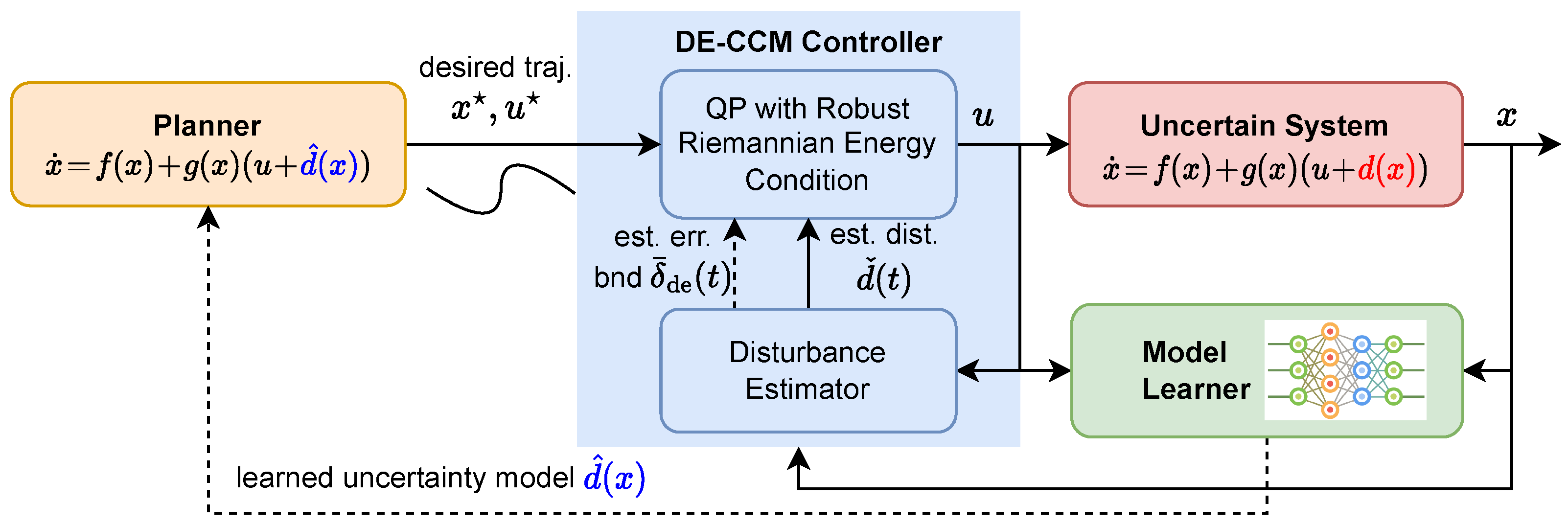
Statement of Contributions: We propose a contraction-based learning control architecture for nonlinear systems with matched uncertainties (depicted in Figure 1). The proposed architecture allows for using different ML tools, e.g., DNNs, for learning the uncertainties while guaranteeing exponential trajectory convergence under certain conditions throughout the learning phase. It leverages a disturbance estimator with a pre-computable estimation error bound (EEB) and a robust Riemann energy condition to compute the control signal. It is empirically shown that learning can help improve the robustness of the controller and facilitate better trajectory planning. We demonstrate the efficacy of the proposed approach using a planar quadrotor example.

Figure 1.
Proposed control architecture incorporating learned dynamics.
This work builds on [16] with several key differences. The authors of [16] introduce a robust tracking controller utilizing CCM and disturbance estimation without involving model learning. In contrast, this work adapts the controller to handle scenarios where machine learning tools are used to learn unknown dynamics, offering tracking performance guarantees throughout the learning phase. Additionally, this research empirically showcases the advantages of integrating learning to improve trajectory planning and strengthen the robustness of the closed-loop system, aspects that are not explored in [16].
Notations. Let and denote the n-dimensional real vector space and the space of real m by n matrices, respectively; 0 and I denote a zero matrix and an identity matrix of compatible dimensions, respectively; and ‖·‖ denotes the ∞-norm and 2-norm of a vector/matrix, respectively. Given a vector y, let denote its ith element. For a vector and a matrix-valued function , let denote the directional derivative of along y. For symmetric matrices P and Q, () means is positive definite (semidefinite); stands for . Finally, we use ⊖ to denote the Minkowski set difference.
2. Preliminaries and Problem Setting
Consider a nonlinear control-affine system
where and are state and input vectors, respectively, and are known functions that are locally Lipschitz, is an unknown function denoting the matched model uncertainties; is assumed to have full column rank for all . Additionally, is a compact set that includes the origin, and is the control constraint set defined as , where and represent the lower and upper bounds of the ith control channel, respectively.
Remark 1.
The matched uncertainty assumption is common in adaptive control [7] or disturbance observer-based control [6] and is made in existing related work.
Assumption 1.
There exist known positive constants , , and such that for any , the following holds:
Remark 2.
Assumption 1 does not assume that the system states stay in (and thus is bounded). We will prove the boundedness of x later in Theorem 1. Assumption 1 merely indicates that is locally Lipschitz with a known bound on the Lipschitz constant and is bounded by a prior known constant in the compact set .
Assumption 1 is not very restrictive as the local Lipschitz bound in for can be conservatively estimated from prior knowledge. Additionally, given the local Lipschitz constant bound and the compact set , we can always derive a uniform bound using Lipschitz property if a bound for for any x in is known. For example, supposing , we have . In practice, leveraging prior knowledge about the system can result in a tighter bound than the one based on Lipschitz continuity. Thus, we assume a uniform bound. Under Assumption 1, it will be shown later (in Section 2.4) that the pointwise value of at any time t can be estimated with pre-computable estimation error bounds (EEBs).
2.1. Learning Uncertain Dynamics
Given a collection of data points with N denoting the number of data points, the uncertain function can be learned using ML tools. For demonstration purposes, we choose to use DNNs, due to their significant potential in dynamics learning attributed to their expressive power and the fact that they have been rarely explored for dynamics learning with safety and/or performance guarantees. Denoting the learned function as and the model error as , the actual dynamics (1) can be rewritten as
where
The learned dynamics can now be represented as
Remark 3.
The above setting includes the special case of no learning, corresponding to .
Note that the performance guarantees provided by the proposed framework are agnostic to the model learning tools used, as long as the following assumption can be satisfied.
Assumption 2.
We are able to obtain a uniform error bound for the learned function , i.e., we could compute a constant such that
Remark 4.
Assumption 2 can be easily satisfied when using a broad class of ML tools. For instance, when Gaussian processes are used, a uniform error bound (UEB) can be computed using the approach in [27]. When using DNNs, we could use spectral-normalized DNNs (SN-DNNs) [28] (to enforce that has a Lispitchz bound in ) and compute the UEB as follows. Obviously, since both and have a local Lipschitz bound in , the model error has a local Lipschitz bound in . As a result, given any point , we have
where is one of the N number of data points. The preceding inequality implies Equation (5) holds with .
2.2. Problem Setting
The learned dynamics Equation (4) (including the special case of ) can be incorporated in a motion planner or trajectory optimizer to plan a desired trajectory to minimize a specific cost function. Suppose Assumptions 1 and 2 hold. The focus of the paper includes
- (i)
- Designing a feedback controller to track the desired state trajectory with guaranteed tracking performance despite the presence of the model error ;
- (ii)
- Empirically demonstrating the benefits of learning in improving the robustness and reducing the cost associated with the actual trajectory.
In the following, we will present some preliminaries on CCM and uncertainty estimation used to build our solution.
2.3. CCM for the Nominal Dynamics
CCM extends contraction analysis [9] to controlled dynamic systems, where the analysis simultaneously seeks a controller and a metric that characterizes the contraction properties of the closed-loop system [10]. According to [10], a symmetric matrix-valued function serves as a strong CCM for the nominal (uncertainty-free) system
in , if there exist positive constants , , and such that
hold for all and .
Assumption 3.
There exists a strong CCM for the nominal system Equation (6) in , i.e., satisfies Equations (7)–(9).
Remark 5.
Similar to the synthesis of Lyapunov functions, given dynamics, a strong CCM can be systematically synthesized using convex optimization, more specially, sum of squares programming [10,12,18].
Given a CCM , a feasible trajectory satisfying the nominal dynamics Equation (6), and the actual state at t, the control signal can be constructed as follows [10,12]. At any , compute a minimal-energy path (termed as geodesic) connecting and , e.g., using the pseudospectral method [29]. Note that the geodesic is always a straight line segment if the metric is constant. Next, compute the Riemann energy of the geodesic, defined as , where . Finally, by interpreting the Riemann energy as an incremental control Lyapunov function, we can construct a control signal such that
where with the dependence on t omitted for brevity, is defined in Equation (6), and . In practice, one may want to compute with a minimal such that Equation (10) holds, which can be achieved by setting with obtained via solving a quadratic programming (QP) problem [10,12]:
at each time t. Problem Equation (11) is commonly referred to as the pointwise minimum-norm control problem and possesses an analytic solution [30]. The performance guarantees provided by the CCM-based controller can be summarized in the following theorem.
Lemma 1
The following lemma from [12] establishes a bound on the tracking control effort from solving Equation (11).
Lemma 2
([12] Theorem 5.2). For all such that for a scalar constant , the control effort from solving Equation (11) is bounded by
where , satisfies , represents the largest eigenvalue, and denotes the smallest non-zero singular value.
2.4. Uncertainty Estimation with Computable Error Bounds
We leverage a disturbance estimator described in [16] to estimate the value of the uncertainty at each time instant. More importantly, an estimation error bound can be pre-computed and systematically reduced by tuning a parameter of the estimator. The estimator comprises a state predictor and an update law. The state predictor is defined by
where denotes the prediction error, is a scalar constant. The estimate, , is given by a piecewise-constant update law:
where T is an estimation sampling time, and . Finally, the value of at time t is estimated as
where is the pseudoinverse of . The following lemma establishes the estimation error bound associated with the disturbance estimator defined by (15) and (16). Lemma 3 can be considered as a simplified version of (Lemma 4 [16]) in the sense that the uncertainty considered in [16] can explicitly depend on both time and states, i.e., represented as , whereas the uncertainty in this paper depends on states only. The proof is similar to that in [16] and is omitted for brevity.
Lemma 3.
Remark 6.
According to Lemma 3, the estimation error after a single sampling interval can be arbitrarily reduced by decreasing T.
Remark 7.
As explained in (Remark 5 [16]), the error bound can be quite conservative primarily due to the conservatives introduced in computing ϕ and . For practical implementation, one could benefit from empirical studies, such as conducting simulations with a selection of user-defined functions of to identify a more refined bound than defined in Equation (19).
3. Disturbance Estimation-Based Contraction Control under Learned Dynamics
This section introduces an approach based on CCM and disturbance estimation to ensure the UES of the uncertain system Equation (2) even when the learned model is poor.
3.1. CCMs and Feasible Trajectories for the True System
The first step is to search for a valid CCM for the uncertain system Equation (2). Due to the special structure of Equation (2) attributed to the matched uncertainty assumption, we have the following lemma. The proof is straightforward by following [15] that considers matched parametric uncertainties and is thus omitted.
Lemma 4.
Define
Equation (22) and Assumption 1 imply that for any . As discussed in Section 2.3, when provided with a CCM and a feasible desired trajectory and , a controller can be designed to exponentially stabilize the actual state trajectory to the desired trajectory . In practice, we only have access to learned dynamics to plan a trajectory. We now present a lemma providing the condition under which planned using the learned dynamics Equation (4) also represents a feasible state trajectory for the true system.
Lemma 5.
3.2. Filtered Disturbance Estimate
Using a small T in the estimation law Equation (16) may introduce high-frequency components into the control signal, which could potentially compromise the robustness of the closed-loop system, e.g., against input delay. This has been demonstrated in the adaptive control literature (Sections 1.3 and 2.1.4 [8]), which shows that a high adaptation rate (corresponding to a small T here) will lead to a reduced time-delay margin. To prevent the high-frequency signal in the estimation loop induced by small T from entering the control loop, we can use a low-pass filter to smooth the estimated uncertainty before using it to compute control signals, as inspired by the adaptive control theory [8]. More specifically, we define the filtered disturbance estimate as
where and denote the Laplace transform and inverse Laplace transform operators, respectively, and is a strictly proper transfer function matrix denoting a stable low pass filter. Notice that is an estimate of the learned model error . Filtering is not necessary because it will not induce high-frequency signals into the control loop, unlike .
For simplicity, we select to be
where () is the filter bandwidth for the jth uncertainty channel. The in Equation (25) can be described by a state-space model , where , and is a matrix with all elements equal to 0 except the element equal to . Define
Leveraging the bound in Equation (19) and solution of state-space systems, we can straightforwardly derive an EEB on , formally stated in the following lemma.
Lemma 6.
Proof.
Notice that Equation (30) can be represented with a state-space model:
where xf(t) is the state vector of the filter. From Equations (19) and (32), we have for any t in ,
where the second inequality is due to the fact that . Additionally, for any t in , since , we have
As a result, we have
On the other hand, since for all t in by assumption, by applying (Lemma A.7.1 [8]) to Equation (31), we have for all t in , where denotes the norm (also known as the induced gain) of a system. Further considering , (due to the specific selected in Equation (25)), Equation (29), and Equation (33), we obtain Equation (27). □
The norm of a linear time-invariant system can be easily computed using the impulse response (Section A.7.1 [8]).
Remark 8.
Remark 9.
As explained in Remark 7, the bound could be quite conservative, which leads to a conservative bound, i.e., , for (defined in Equation (30)). Additionally, the bound on can also be quite conservative due to the use of the norm of a system and the norms of inputs and outputs, e.g., characterized by (Lemma A.7.1 [8]). As a result, the bound is most likely rather conservative. For practical implementation, one could leverage some empirical study, e.g., doing simulations under a few user-selected functions of and and determining a tighter bound based on the simulation results.
Remark 10.
For many control techniques, including a low-pass filter will induce phase delay and may damage system performance and/or robustness. However, this is not true for adaptive or uncertainty estimation-based control. As demonstrated in the adaptive control literature [8], including a low-pass filter with properly designed bandwidth can actually improve system robustness, e.g., against input delay. Simulation tests in Appendix A indicate that this is also true for the proposed control technique. Additionally, the low-pass filter is only applied to the estimate of the learned model error (i.e., ), and influences the estimation error bound. Such an influence will decrease when the learned model improves.
3.3. Robust Riemann Energy Condition under Learned Dynamics
Section 2.3 demonstrates that with a nominal system and a CCM established for it, one can devise a controller to limit the rate of decrease of the Riemann energy, as described by Equation (10). Now, given uncertain dynamics with the learned model in Equation (2), and the planned trajectory using the learned model, under condition Equation (23), condition Equation (10) now becomes
where denotes the true dynamics evaluated at , and denotes the learned dynamics defined in Equation (3). Obviously, Equation (34) is not implementable since it depends on the uncertainty . However, by estimating the value of at each time t with a computable estimation error bound, we could establish a robust condition for Equation (34) [16]. In particular, consider the filtered disturbance estimate introduced in Section 3.2 that estimates as at each time t with an error bound defined in Equation (27). Then, a sufficient condition for Equation (34) can be obtained as
where Moreover, since satisfies the CCM conditions (7), (8), and (9), control input that satisfies (35) will exist for any , irrespective of the size of , in the absence of control limits, i.e., . We call condition Equation (35) the robust Riemann energy (RRE) condition.
Remark 11.
From Section 2.4 and Section 3.3, we see that the disturbance estimate provided by Equations (15) and (16) and incorporated in the RRE condition Equation (35) is the discrepancy between the true dynamics and the nominal dynamics without the learned model (i.e., ). Alternatively, we can easily adapt the estimation law Equations (15) and (16) to estimate (i.e., the discrepancy between learned dynamics Equation (4) and true dynamics) and adjust the RRE condition accordingly. However, as characterized in Equation (19), the EEB depends on the local Lipschitz bound of the uncertainty to be estimated, which indicates that a Lipschitz bound for is needed to establish the EEB for it.
3.4. Guaranteed Trajectory Tracking under Learned Dynamics
Similar to Section 2.3, we can compute a control input at each time t to satisfy the RRE condition Equation (35). In practice, one may want to compute with a minimal , which can be achieved by setting with obtained via solving a QP problem:
at each , where
and Equation (37) is an equivalent representation of Equation (35), is the filtered disturbance estimate via Equations (15)–(17) and (24), is defined in Equation (27), and is defined in Equation (3). Problem Equation (36) is commonly referred to as a min-norm problem and can be analytically solved by [30]
Remark 12.
The proposed controller is inspired by the adaptive control theory [8]. In fact, we adopt the estimation mechanism (the PWCE law in Equations (15) and (16)) used within an controller. However, instead of directly canceling the estimated disturbance as one would do with an controller, the proposed approach incorporates the estimated uncertainty and the EEBs into the robust Riemann energy condition Equation (37) to compute the control signal, which ensures exponential convergence of actual trajectories to desired ones.
The following lemma establishes a bound on the control input given by solving Equation (36).
Lemma 7.
Proof.
The main theoretical result of the paper is stated below.
Theorem 1.
Consider an uncertain system Equation (2) with learned dynamics . Suppose Assumptions 1 and 2 hold and Assumption 3 holds with positive constants , , and λ. Furthermore, suppose the initial state vector and a continuous trajectory () planned using the learned dynamics Equation (4) satisfy Equations (23), (43) and (44),
for any , where denotes the interior of a set, is defined in Equation (40) with
for an arbitrary . Then, the control law with solving Equation (36) ensures that and for all ,
and universally exponentially stabilizes the system Equation (2) in the sense that Equation (13) holds.
Proof.
Since Assumption 2 holds, we have since . The EEB in Equation (27) holds for due to the fact that . As a result, the bound in Equation (40) holds for with , which, together with Equation (43), implies .
We next prove and for all by contradiction. Assume this is not true. Since and are continuous ( is continuous because is continuous, and is also continuous according to Equation (36)), there must exist a time such that
Now, examine the evolution of the system within the interval . Due to Equation (46), the error bound in Equation (19) holds within . Also, notice that condition Equation (23) ensures that represents a feasible trajectory for the uncertain system Equation (2) with input constraints according to Lemma 5. Therefore, the control law given by Equation (36) guarantees the fulfillment of of the RRE condition Equation (35), and, consequently, of condition Equation (34), which further implies Equation (10), or equivalently,
for all t in . Lemma 1 and Equation (48) indicate that , which, together with Equation (44), implies that stays in the interior of , . Considering that is continuous, we have , contradicting the first condition in Equation (47). As a result, we have
Now, consider the second condition in Equation (47). Condition Equation (48) implies for any t in , where denotes the Riemann distance between and x and is defined in Equation (45). Considering the continuity of and , we have
Due to Equation (49) and for all (from Equation (46)), it follows from Lemma 3 that the error bound in Equation (19) holds in , which, together with Equation (49), implies the filter-dependent error bound in Equation (27) holds in . This fact, along with Equation (50), indicates that Equation (40) holds, i.e., , for all t in . Further considering Equation (43), we have for all t in , which, together with Equation (49), contradicts Equation (47). Therefore, we conclude that and for all . From the development of the proof, it is clear that the the UES of the closed-loop system in with the control law given by the solution of Equation (36) is achieved. □
Remark 13.
Theorem 1 asserts that, under specific conditions, the proposed controller ensures exponential convergence of the actual state trajectory to a desired trajectory that may be planned using a potentially poorly learned model. On the other hand, the improved accuracy of the learned model reduces the error bound and thus the EEB , and improve the robustness of the controller, as will be demonstrated by simulation results in Section 4.
Remark 14.
The exponential convergence assurance described in Theorem 1 relies on a continuous-time implementation of the controller. However, in practical applications, controllers are typically implemented on digital processors using fixed sampling times. Consequently, the property of exponential convergence may be slightly compromised, as noted in Section 4.
3.5. Discussion
With consideration of Equation (40), condition Equation (43) in Theorem 1 requires that, when planning nominal input trajectories, enough control authority should be left for the control law defined by Equation (36). Additionally, the control effort bound depends on the error bound of the learned model, ; a poorly learned model with large will lead to large , making it challenging to satisfy Equation (43).
Although Theorem 1 only mentions the trajectory tracking performance, we will empirically show the benefits of learning in facilitating better trajectory planning and improving the robustness of the controller in Section 4.
4. Simulation Results
We validate the proposed learning control approach on a 2D quadrotor introduced in [12]. We selected this example because the 2D quadrotor, although simpler than a 3D quadrotor, presents significant control challenges due to its nonlinear and unstable dynamics. Additionally, it offers a suitable scenario for demonstrating the applicability of the proposed control architecture, specifically, maintaining safety and reducing energy consumption in the presence of disturbances. Matlab codes can be found at github.com/boranzhao/de-ccm-w-learning, https://github.com/boranzhao/de-ccm-w-learning, accessed on 12 May 2024. The dynamics of the vehicle are given by
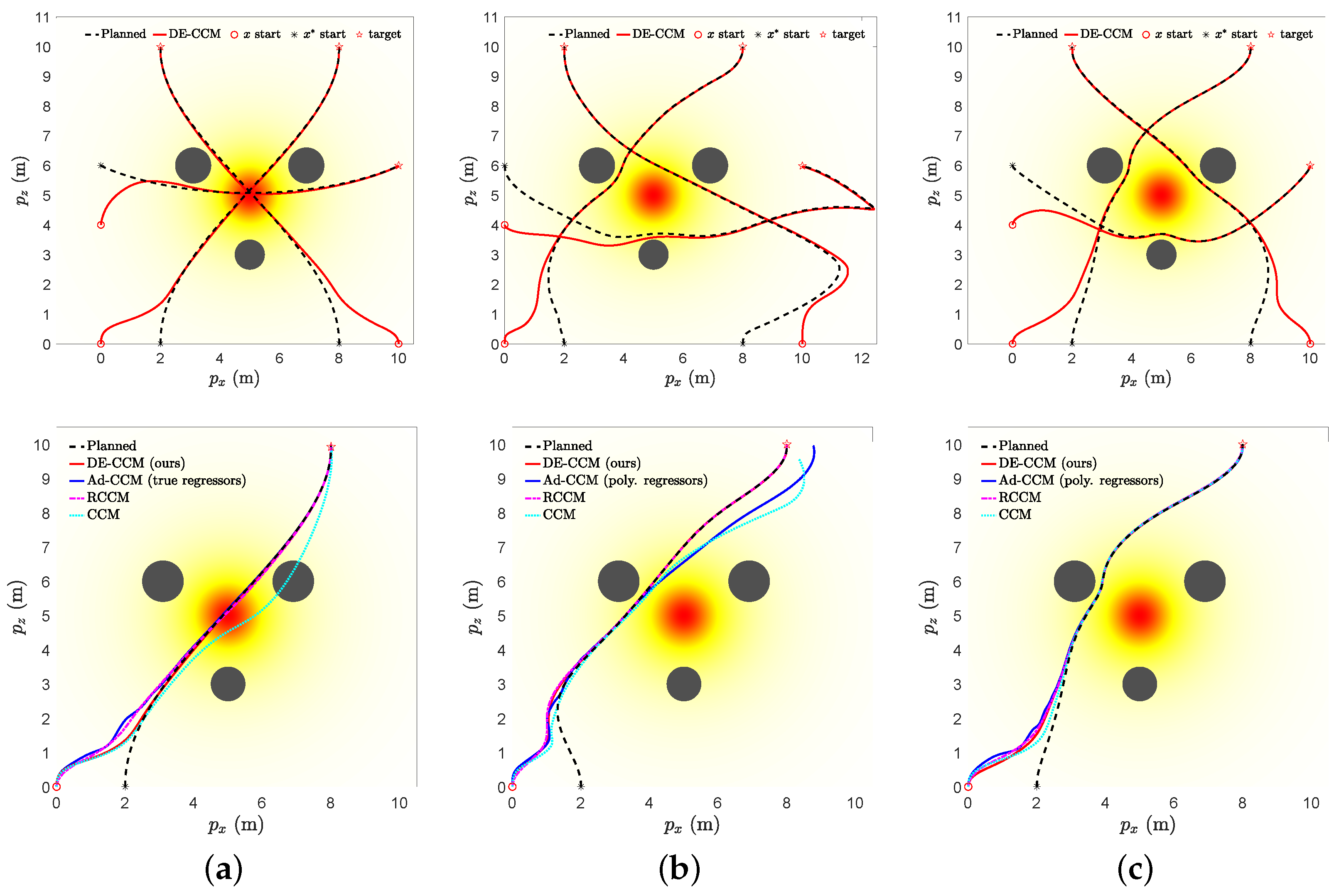
where and represent the positions in x and z directions, respectively, and denote the lateral velocity and velocity along the thrust axis in the body frame; is the angle between the x direction of the body frame and the x direction of the inertia frame. The input vector contains the thrust force produced by the two propellers; m and J represent the mass and moment of inertia about the out-of-plane axis, respectively; l denotes the distance between each propeller and the vehicle center, and signifies the unknown disturbances exerted on the propellers. Specific parameter values are assigned as follows: kg, , and m. We choose to be , where represents the disturbance intensity whose values in a specific location are denoted by the color at this location in Figure 2. We consider three navigation tasks with different start and target points, while avoiding the three circular obstacles, as illustrated in Figure 2. The planned trajectories were computed using OptimTraj [31] to minimize a cost function , where denotes the arrival time. The actual start points for Tasks 1∼3 were intentionally set to be different from the desired ones used for trajectory planning.

Figure 2.
(Top): Planned and executed trajectories under our proposed DE-CCM for Tasks 1∼3 under different learning scenarios. (Bottom): Tracking performance of DE-CCM, Ad-CCM [15], RCCM (which can be seen as a special case of DE-CCM with uncertainty estimate set to 0), and CCM for Task 1 under different learning scenarios. Start points of planned and actual trajectories are intentionally set to be different to reveal the transient response under different scenarios.
4.1. Control Design
For computing a CCM, we parameterized the CCM W by and , and set the convergence rate to 0.8. Additionally, we enforced the constraints: , . More details about synthesizing the CCM and computing the geodesic can be found in [18]. All the subsequent computations and simulations except DNN training (which was done in Python using PyTorch) were done in MATLAB R2021b. For estimating the disturbance using Equations (15)–(17), we set . It is straightforward to confirm that , , and (due to the constant nature of B) satisfy Equation (2). By discretizing the space into a grid, one can determine the constant in Lemma 3 to be . Based on Equation (19), to achieve an error bound , the estimation sampling time needs to satisfy s. However, as mentioned in Remark 7, the error bound calculated from Equation (19) might be overly conservative. Through simulations, we determined that a sampling time of s was sufficient to achieve the desired error bound and thus set s.
4.2. Performance and Robustness across Learning Transients
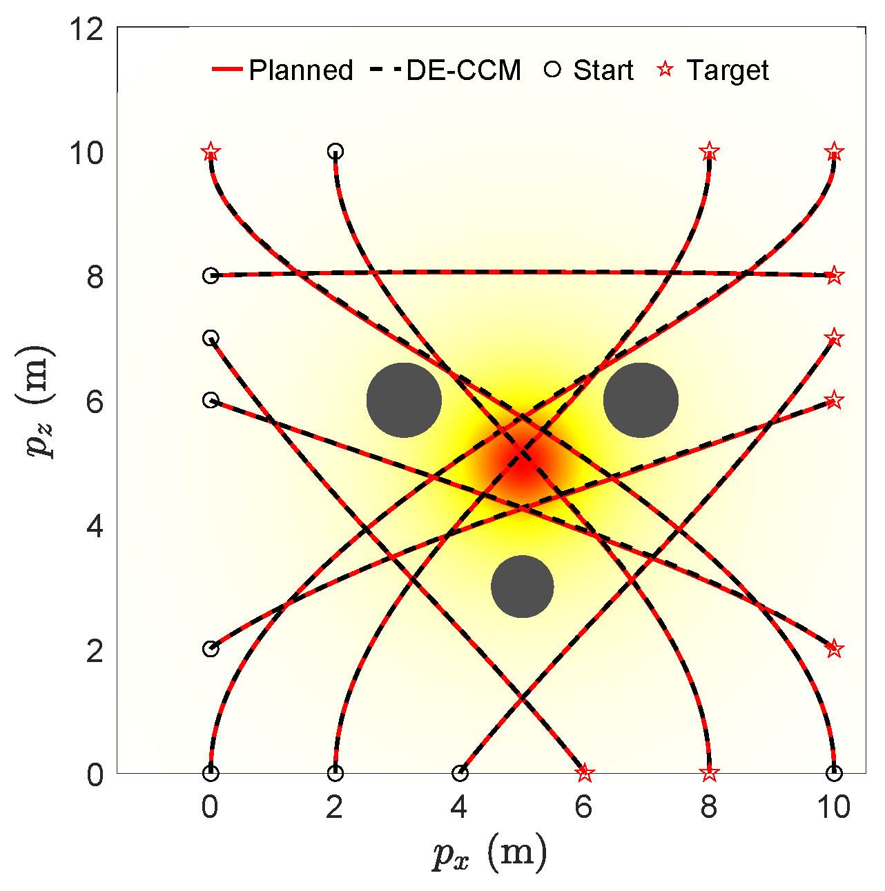
Figure 2 (top) illustrates the planned and actual trajectories under the proposed controller utilizing the RRE condition and disturbance estimation (referred to as DE-CCM), in the presence of no, moderate, and good learned model for uncertain dynamics. For these results, we did not low-pass filter the estimated uncertainty, which is equivalent to setting in Equation (24). Spectral-normalized DNNs [28] (Remark 4) with four inputs, two outputs, and four hidden layers were used for model learning. For training data collection, we planned and executed nine trajectories with different start and end points, as shown in Figure 3. The data collected during the execution of these trajectories were used to train the moderate model. However, these nine trajectories were still not enough to fully explore the state space. Sufficient exploration of the state space is necessary to learn a good uncertainty model. Thanks to the performance guarantee, the DE-CCM controller facilitates safe exploration, as demonstrated in Figure 3. For illustration purposes, we directly used the true uncertainty model to generate the data and used the generated data for training, which yielded the good model.
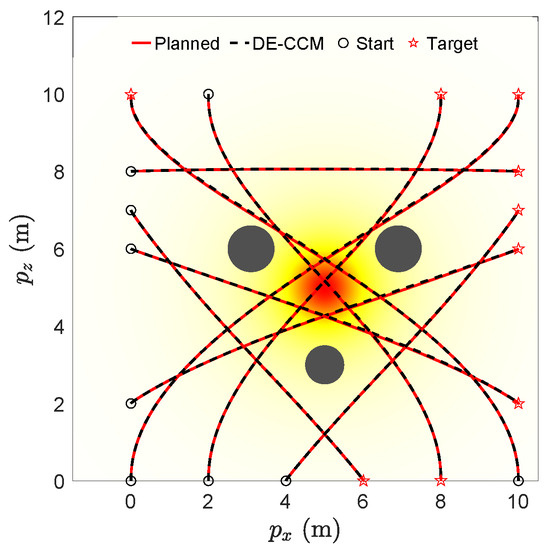
Figure 3.
Safe exploration of the state space for learning uncertain dynamics under DE-CCM.
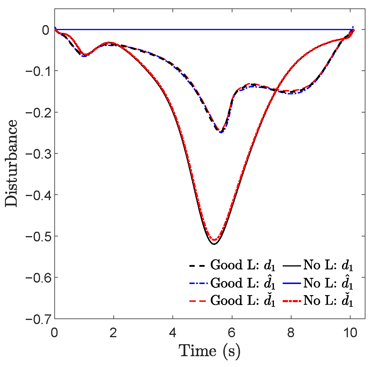
As depicted in Figure 2, the actual trajectories generated by DE-CCM exhibited expected convergence towards the desired trajectories during the learning phase across all three tasks. The minor deviations observed between the actual and desired trajectories under DE-CCM can be attributed to the finite step size used in the ODE solver employed for simulations (refer to Remark 14). The planned trajectory for Task 2 in the moderate learning case seemed unusual near the end point. This is because the learned model was not accurate in the area due to a lack of sufficient exploration. However, with the DE-CCM controller, the quadrotor was still able to track the trajectory. Figure 4 depicts the trajectories of true, learned, and estimated disturbances in the presence of no and good learning for Task 1; the trajectories for Tasks 2 and 3 are similar and thus omitted. One can see that the estimated disturbances were always fairly close to the true disturbances. Also, the area with high disturbance intensity was avoided under good learning, which explains the smaller disturbance encountered.
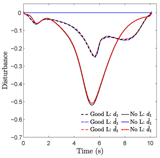
Figure 4.
Trajectories of true, learned, and estimated disturbances in the presence of no and good learning for Task 1. The notations , , and denote the first element of d, , and , respectively.
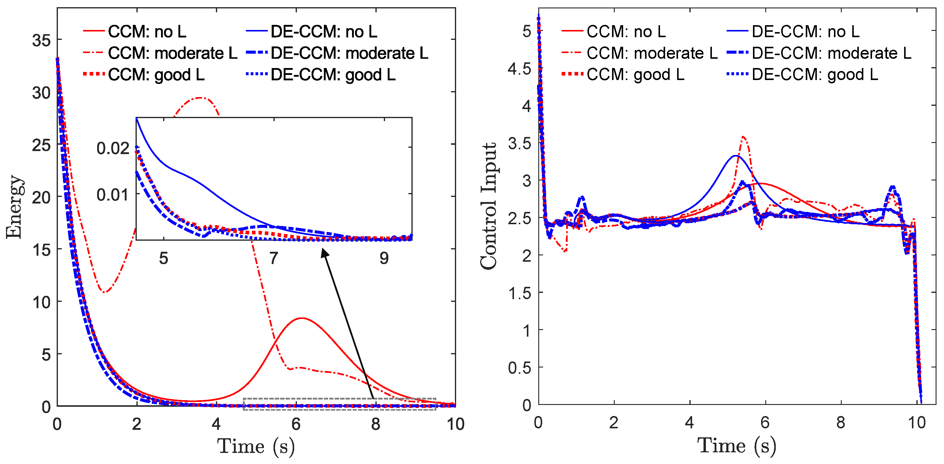
Figure 5 shows trajectories of Riemann energy in the presence of no and good learning for Task 1; the trajectories for Tasks 2 and 3 are similar and thus omitted. It is evident that under DE-CCM decreased exponentially across all scenarios, irrespective of the quality of the learned mode. To compare, we implemented three additional controllers, namely, a vanilla CCM controller that disregards the uncertainty or learned model error, an adaptive CCM (Ad-CCM) controller from [15] with true and polynomial regressors, and a robust CCM (RCCM) controller that can be seen as a specific case of a DE-CCM controller with the uncertainty estimate equal to zero and the EEB equal to the disturbance bound . The Ad-CCM controller [15] needs a parametric structure for the uncertainty in the form of , with being a known regressor matrix and being the vector of unknown parameters. For the no-learning case, we assume that we know the regressor matrix for the original uncertainty . For the learning cases, since we do not know the regressor matrix for the learned model error , we used a second-order polynomial regressor matrix:
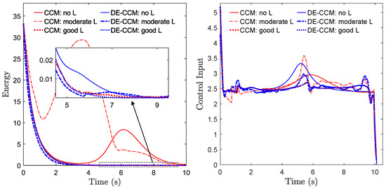
Figure 5.
Trajectories of Riemann energy (left) and the first element of control input (right), i.e., , in the presence of no, poor, and good learning for Task 1.
Figure 2 (bottom) shows the tracking control performances yielded by these additional controllers for Task 1 under different learning scenarios. The observed trajectories resulting from the CCM controller showed significant deviations from the planned trajectories and occasionally encountered collisions with obstacles, except in the case of good learning. Additionally, Ad-CCM yielded poor tracking performance under the moderate learning case. The poor performance could be attributed to the fact that the uncertainty may not have a parametric structure, or, even if it does, the selected regressor may not be sufficient to represent it. RCCM achieved similar performance as compared to the proposed method, but shows weaker robustness against control input delays, as demonstrated later.
4.3. Improved Planning and System Robustness with Learning
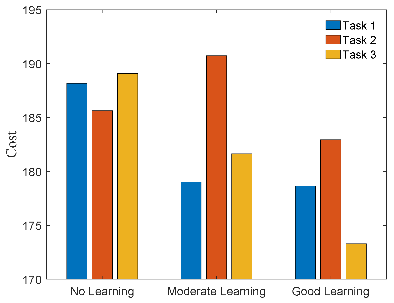
Figure 6 shows the costs J associated with the actual trajectories achieved by DE-CCM under different learning qualities. As expected, the good model helped plan better trajectories, leading to reduced costs for all three tasks. It is not a surprise that the poor and moderate models led to a temporal increase in the costs for some tasks. In practice, we may not use the poorly learned model directly for planning trajectories. DE-CCM ensures that in case one really does so, the planned trajectories can still be tracked well.
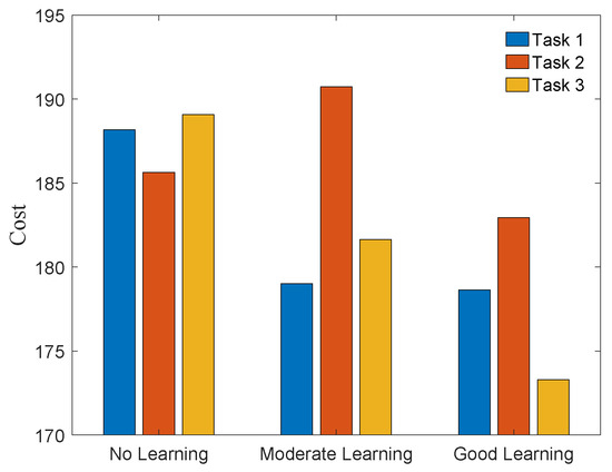
Figure 6.
Costs of actual trajectories achieved by DE-CCM throughout the learning phase.
The role of the low-pass filter in protecting system robustness under the no learning case is illustrated in Appendix A. We next tested the robustness of RCCM and DE-CCM against input delays under different learning scenarios. Note that, unlike linear systems for which gain and phase margins are commonly used as robustness criteria, we often evaluate the robustness of nonlinear systems in terms of their tolerance for input delays. Under an input delay of , plant dynamics Equation (1) becomes . For these experiments, we leveraged a low-pass filter to filter the estimated disturbance following Equation (24). In principle, the EEB of 0.1 used in the previous experiments would not hold anymore, as the presence of the filter would lead to a larger error bound according to Equation (27). However, we kept using the same EEB of 0.1, as the theoretical bound according to Equation (27) could be quite conservative. The Riemann energy, which indicates the tracking performance for all states, is shown in Figure 7. One can see that, under both delay cases, DE-CCM achieves smaller and less oscillatory Riemann energy, indicating better robustness and tracking performance, compared to RCCM.
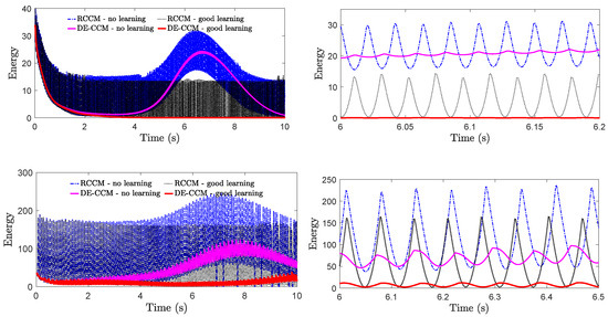
Figure 7.
Riemann energy yielded by DE-CCM and RCCM under different learning cases with an input delay of 10 ms (top) and 30 ms (bottom). Note that the plots on the right are zoomed-in versions of the corresponding plots on the left. Learning improves the robustness of both DE-CCM and RCCM against input delays.
Additionally, the robustness of DE-CCM against input delays in the presence of good learning is significantly improved compared to the no-learning case, which illustrates the benefits of incorporating learning. This can be explained as follows. The input delay may cause the disturbance estimate to be highly oscillatory and a large discrepancy between and . The low pass filter can filter out the high-frequency oscillatory component of . Under good learning, according to Equation (24), the learned model approaches the true uncertainty ; as a result, the filtered disturbance estimate defined in Equation (24) can be much closer to , leading to improved robustness and performance, compared to no and moderate learning cases.
5. Conclusions
This paper presents a disturbance estimation-based contraction control architecture that allows for using model learning tools (e.g., a neural network) to learn uncertain dynamics while guaranteeing exponential trajectory convergence during learning transients under certain conditions. The architecture uses a disturbance estimator to estimate the value of the uncertainty, i.e., the difference between nominal dynamics and actual dynamics, with pre-computable estimation error bounds (EEBs), at each time instant. The learned dynamics, the estimated disturbances, and the EEBs are then incorporated into a robust Riemann energy condition, which is used to compute the control signal that guarantees exponential convergence to the desired trajectory throughout the learning phase. On the other hand, we show that learning can facilitate better trajectory planning and improve the robustness of the closed-loop system, e.g., against input delays. The proposed framework is validated on a planar quadrotor example.
Future directions could involve addressing broader uncertainties, especially unmatched uncertainties prevalent in practical systems, minimizing the conservatism of the estimation error bound, and demonstrating the efficacy of the proposed control framework with alternative model learning tools.
Author Contributions
Conceptualization, P.Z., A.G., Y.C. and N.H.; methodology, P.Z. and Z.G.; software, P.Z., Z.G. and H.K.; validation, P.Z. and Z.G.; formal analysis: P.Z.; investigation, resources, P.Z.; data curation, P.Z. and Z.G.; writing—original draft preparation, P.Z., Z.G. and Y.C.; writing—review and editing, P.Z.; supervision, N.H.; funding acquisition, P.Z. and N.H. All authors have read and agreed to the published version of the manuscript.
Funding
This research was funded in part by NASA through the ULI grant #80NSSC22M0070, and in part by NSF under the RI grant #2133656.
Data Availability Statement
All data are contained within this article and cited references.
Conflicts of Interest
The authors declare no conflicts of interest.
Appendix A. Ablation Study on the Role of the Low-Pass Filter
We tested the performance of DE-CCM under different filter bandwidths in the presence of a 10 ms input delay. The estimation error bound was fixed to 0.1 for all test cases. The results are shown in Figure A1. It is evident that the low-pass filter helps protect the robustness of the DE-CCM against input delay. Moreover, this protection decreases when the filter bandwidth increases. Note that the no-filter case can be considered equivalent to a filter with infinitely high bandwidth. We also repeated the above tests but without injecting input delay, and we did not notice much difference among the different filter cases in terms of both tracking performance and control inputs.
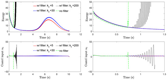
Figure A1.
Riemann energy (top) and control input (bottom) yielded by DE-CCM under different filters in the presence of 10 ms input delay. The plots on the right are zoomed-in versions of the corresponding plots on the left; denotes the bandwidth of a first-order low-pass filter for both control input channels. Simulations for and no-filter cases had to be pre-emptively stopped due to too much deviation of actual states from nominal states, which rendered computation of the geodesic (see Section 2.3) infeasible.
References
- Zhou, K.; Doyle, J.C. Essentials of Robust Control; Prentice Hall: Upper Saddle River, NJ, USA, 1998. [Google Scholar]
- Edwards, C.; Spurgeon, S. Sliding Mode Control: Theory and Applications; CRC Press: Boca Raton, FL, USA, 1998. [Google Scholar]
- Mayne, D.Q.; Seron, M.M.; Raković, S. Robust model predictive control of constrained linear systems with bounded disturbances. Automatica 2005, 41, 219–224. [Google Scholar] [CrossRef]
- Mayne, D.Q. Model predictive control: Recent developments and future promise. Automatica 2014, 50, 2967–2986. [Google Scholar] [CrossRef]
- Han, J. From PID to active disturbance rejection control. IEEE Trans. Ind. Electron. 2009, 56, 900–906. [Google Scholar] [CrossRef]
- Chen, W.H.; Yang, J.; Guo, L.; Li, S. Disturbance-observer-based control and related methods—An overview. IEEE Trans. Ind. Electron. 2015, 63, 1083–1095. [Google Scholar] [CrossRef]
- Ioannou, P.A.; Sun, J. Robust Adaptive Control; Dover Publications, Inc.: Mineola, NY, USA, 2012. [Google Scholar]
- Hovakimyan, N.; Cao, C. L1 Adaptive Control Theory: Guaranteed Robustness with Fast Adaptation; Society for Industrial and Applied Mathematics: Philadelphia, PA, USA, 2010. [Google Scholar]
- Lohmiller, W.; Slotine, J.J.E. On contraction analysis for non-linear systems. Automatica 1998, 34, 683–696. [Google Scholar] [CrossRef]
- Manchester, I.R.; Slotine, J.J.E. Control contraction metrics: Convex and intrinsic criteria for nonlinear feedback design. IEEE Trans. Autom. Control. 2017, 62, 3046–3053. [Google Scholar] [CrossRef]
- Tsukamoto, H.; Chung, S.J. Robust controller design for stochastic nonlinear systems via convex optimization. IEEE Trans. Autom. Control 2020, 66, 4731–4746. [Google Scholar] [CrossRef]
- Singh, S.; Landry, B.; Majumdar, A.; Slotine, J.J.; Pavone, M. Robust feedback motion planning via contraction theory. Int. J. Robot. Res. 2023, 42, 655–688. [Google Scholar] [CrossRef]
- Tsukamoto, H.; Chung, S.J. Neural contraction metrics for robust estimation and control: A convex optimization approach. IEEE Control Syst. Lett. 2020, 5, 211–216. [Google Scholar] [CrossRef]
- Sun, D.; Jha, S.; Fan, C. Learning certified control using contraction metric. In Proceedings of the Conference on Robot Learning, virtual, 16–18 November 2020. [Google Scholar]
- Lopez, B.T.; Slotine, J.J.E. Adaptive nonlinear control with contraction metrics. IEEE Control Syst. Lett. 2020, 5, 205–210. [Google Scholar] [CrossRef]
- Zhao, P.; Guo, Z.; Hovakimyan, N. Robust Nonlinear Tracking Control with Exponential Convergence Using Contraction Metrics and Disturbance Estimation. Sensors 2022, 22, 4743. [Google Scholar] [CrossRef] [PubMed]
- Lakshmanan, A.; Gahlawat, A.; Hovakimyan, N. Safe feedback motion planning: A contraction theory and L1-adaptive control based approach. In Proceedings of the 2020 59th IEEE Conference on Decision and Control (CDC), virtual, 14–18 December 2020; pp. 1578–1583. [Google Scholar]
- Zhao, P.; Lakshmanan, A.; Ackerman, K.; Gahlawat, A.; Pavone, M.; Hovakimyan, N. Tube-certified trajectory tracking for nonlinear systems with robust control contraction metrics. IEEE Robot. Autom. Lett. 2022, 7, 5528–5535. [Google Scholar] [CrossRef]
- Manchester, I.R.; Slotine, J.J.E. Robust control contraction metrics: A convex approach to nonlinear state-feedback H∞ control. IEEE Control Syst. Lett. 2018, 2, 333–338. [Google Scholar] [CrossRef]
- Tsukamoto, H.; Chung, S.J.; Slotine, J.J.E. Contraction theory for nonlinear stability analysis and learning-based control: A tutorial overview. Annu. Rev. Control 2021, 52, 135–169. [Google Scholar] [CrossRef]
- Khojasteh, M.J.; Dhiman, V.; Franceschetti, M.; Atanasov, N. Probabilistic safety constraints for learned high relative degree system dynamics. In Proceedings of the 2nd Conference on Learning for Dynamics and Control (L4DC), virtual, 10–11 June 2020; pp. 781–792. [Google Scholar]
- Berkenkamp, F.; Schoellig, A.P. Safe and robust learning control with Gaussian processes. In Proceedings of the Second Euro-China Conference on Intelligent Data Analysis and Applications ECC, Linz, Austria, 15–17 July 2015; pp. 2496–2501. [Google Scholar]
- Chou, G.; Ozay, N.; Berenson, D. Model error propagation via learned contraction metrics for safe feedback motion planning of unknown systems. In Proceedings of the 60th IEEE Conference on Decision and Control (CDC), Austin, TX, USA, 14–17 December 2021; pp. 3576–3583. [Google Scholar]
- Joshi, G.; Chowdhary, G. Deep model reference adaptive control. In Proceedings of the 2019 IEEE 58th Conference on Decision and Control (CDC), Nice, France, 11–13 December 2019; pp. 4601–4608. [Google Scholar]
- Sun, R.; Greene, M.L.; Le, D.M.; Bell, Z.I.; Chowdhary, G.; Dixon, W.E. Lyapunov-based real-time and iterative adjustment of deep neural networks. IEEE Control Syst. Lett. 2021, 6, 193–198. [Google Scholar] [CrossRef]
- Shi, G.; Shi, X.; O’Connell, M.; Yu, R.; Azizzadenesheli, K.; Anandkumar, A.; Yue, Y.; Chung, S.J. Neural lander: Stable drone landing control using learned dynamics. In Proceedings of the International Conference on Robotics and Automation (ICRA), Montreal, QC, Canada, 20–24 May 2019; pp. 9784–9790. [Google Scholar]
- Lederer, A.; Umlauft, J.; Hirche, S. Uniform error bounds for gaussian process regression with application to safe control. Adv. Neural Inf. Process. Syst. 2019, 32, 657–667. [Google Scholar]
- Miyato, T.; Kataoka, T.; Koyama, M.; Yoshida, Y. Spectral normalization for generative adversarial networks. In Proceedings of the ICLR, Vancouver, BC, Canada, 30 April–3 May 2018. [Google Scholar]
- Leung, K.; Manchester, I.R. Nonlinear stabilization via control contraction metrics: A pseudospectral approach for computing geodesics. In Proceedings of the American Control Conference, Seattle, WA, USA, 24–26 May 2017; pp. 1284–1289. [Google Scholar]
- Freeman, R.; Kokotovic, P.V. Robust Nonlinear Control Design: State-Space and Lyapunov Techniques; Springer Science & Business Media: Boston, MA, USA, 2008. [Google Scholar]
- Kelly, M. An introduction to trajectory optimization: How to do your own direct collocation. SIAM Rev. 2017, 59, 849–904. [Google Scholar] [CrossRef]

Disclaimer/Publisher’s Note: The statements, opinions and data contained in all publications are solely those of the individual author(s) and contributor(s) and not of MDPI and/or the editor(s). MDPI and/or the editor(s) disclaim responsibility for any injury to people or property resulting from any ideas, methods, instructions or products referred to in the content. |
© 2024 by the authors. Licensee MDPI, Basel, Switzerland. This article is an open access article distributed under the terms and conditions of the Creative Commons Attribution (CC BY) license (https://creativecommons.org/licenses/by/4.0/).