Abstract
PyNeb is a Python package widely used to model emission lines in gaseous nebulae. We take advantage of its object-oriented architecture, class methods, and historical atomic database to structure a practical environment for atomic data assessment. Our aim is to reduce the uncertainties in the parameter space (line ratio diagnostics, electron density and temperature, and ionic abundances) arising from the underlying atomic data by critically selecting the PyNeb default datasets. We evaluate the questioned radiative-rate accuracy of the collisionally excited forbidden lines of the N- and P-like ions (O ii, Ne iv, S ii, Cl iii, and Ar iv), which are used as density diagnostics. With the aid of observed line ratios in the dense NGC 7027 planetary nebula and careful data analysis, we arrive at emissivity ratio uncertainties from the radiative rates within 10%, a considerable improvement over a previously predicted 50%. We also examine the accuracy of an extensive dataset of electron-impact effective collision strengths for the carbon isoelectronic sequence recently published. By estimating the impact of the new data on the pivotal [N ii] and [O iii] temperature diagnostics and by benchmarking the collision strength with a measured resonance position, we question their usefulness in nebular modeling. We confirm that the effective-collision-strength scatter of selected datasets for these two ions does not lead to uncertainties in the temperature diagnostics larger than 10%.
1. Introduction
PyNeb1 [1,2] is a Python package for the analysis of emission lines in gaseous nebulae, namely H ii regions and planetary nebulae. These lines are used to diagnose the nebular plasma conditions (typical electron densities cm and temperatures from a few thousand to tens of thousands Kelvin) and to ultimately estimate chemical abundances. Due to reliable observations in the infrared, optical, and ultraviolet and well-constrained plasma models, the ubiquitous galactic and extragalactic nebulae have become abundance tracers of choice to study cosmic chemical evolution [3].
The atomic radiative and collisional rates in nebular models are mainly determined by computation, where inherent theoretical difficulties and computational limitations compromise accuracy. For instance, most collisionally excited lines are dipole forbidden or semi-forbidden (), for which the theoretical A-values and collision strengths must take into account fundamental electron-correlation and relativistic effects; additionally, for the forbidden transitions in particular, the collision strengths are dominated by intricate series of resonances [4,5]. For radiative recombination lines, low-temperature dielectronic recombination rates are also sensitive to near-threshold resonances, whose energy positions are model dependent (e.g., vs. intermediate coupling ionic models) and lack experimental benchmarks [6]. It is noteworthy that the development of the codes to calculate relativistic atomic structure and electron–ion scattering has been in great part driven by the stringent requirements of these transition rates, which in many cases are still to converge to the desirable accuracy despite large calculations [7]. With the intention of promoting a fluid and constructive interaction between atomic data producers and users in nebular physics, for which we have well-recognized contributions [8,9], we have undertaken the present atomic data assessment joint project.
The deep-seated dependence of nebular spectral models on the underlying atomic parameters has encouraged the implementation of databases that have become standard references (e.g., [10,11]) or an integral part of spectral modeling tools such as chianti2 [12,13], cloudy3 [14], xstar4 [15], and PyNeb. Regarding modeling codes, periodic atomic data curation (i.e., upgrading, selection, and assessment) has become a major determinant of their usefulness, PyNeb having the distinctive advantage of keeping a historical database with all the available radiative and collisional datasets rather than discarding data when upgrading. This data-curation strategy allows modelers to estimate the uncertainties of the plasma diagnostics and chemical abundances arising from the scatter of the atomic parameters and also provides a suitable environment for atomic data assessment, the central topic of the present report. This capability of the package is conceptually similar to AtomPy [11,16], but supported by a battery of class methods that facilitate the data revision procedures.
2. PyNeb Package
The PyNeb Python package [2] is tailored to derive the nebular plasma conditions (electron temperature and density) and relative chemical abundances by comparing observed line intensities with computed emissivities, for which it provides a variety of extinction laws, ionization correction factors (ICF), diagnostic plots, and Balmer/Paschen jump temperature determinations. Modules, documentation, historic versions and logs, and notebooks can be accessed from the PyNeb GitHub repository5. The current version used in this paper is 1.1.13.
For an -level ionic model and a given electron temperature and density, PyNeb solves the equilibrium equations to determine the level populations, critical densities, and line emissivities, which lead to plasma diagnostics based on observed line ratios. For this purpose, it can upload and manage observational datasets to finally obtain the ionic abundances and, by means of ICF, the elemental abundances. Since the default atomic datasets can be readily changed and updated, the package furnishes plots to compare the atomic parameters from different sources.
Since we are mainly concerned in this report with collisionally excited lines, we recall the basic formalism used by PyNeb to compute the emissivities to derive abundances from such lines. Emissivities for collisionally excited lines are obtained by solving the equations of statistical equilibrium for an -level ionic system:
assuming that:
where is the total ion density, the electron density, the level population of the ith level, and the radiative transition rate for levels . The electron-impact de-excitation rate coefficient is usually expressed in terms of the effective collision strength as:
being the statistical weight of the upper level. The excitation rate coefficient can be obtained from the detailed balance relation:
where is the Boltzmann factor. It must be noted that for historic reasons [17], the effective collision strength , i.e., the temperature-dependent Maxwell-averaged collision strength , is often referred to in the nebular community simply as the collision strength .
The line emissivity is given by:
and for cospatial ions, the emissivity ratio of a pair of optically thin lines is equal to the line intensity ratio, allowing the formulation of plasma diagnostics to determine the electron density and temperature. Furthermore, for an ion emitting a line with wavelength and intensity , it can be shown that:
an expression that leads to the ionic abundance. The elemental abundance is then given by the sum:
that assumes an ionization correction factor for the unseen ionic species ( being the set of observed ionic species).
Figure 1 gives an outline of the PyNeb object-oriented architecture, where the ion object is represented by the Atom and RecAtom classes. They offer a set of methods to determine the temperature and density (getTemDen), emissivities (getEmissivity), and ionic abundances (getionAbundance) through the atomicData manager. In the present work, we use the graphic methods of DataPlot to examine the atomic data scatter. The RecAtom class computes emissivities for recombination lines by table interpolation or a fitting formula using eponymous methods to obtain the ionic abundance. Useful stacks of emissivity grids can be generated with the emisGrid class and multi-diagnostic ratios with Diagnostics. Astronomical observations are managed with the Observation class, and diagnostic plots can be devised by means of the Observation, Diagnostics, and emisGrid classes.
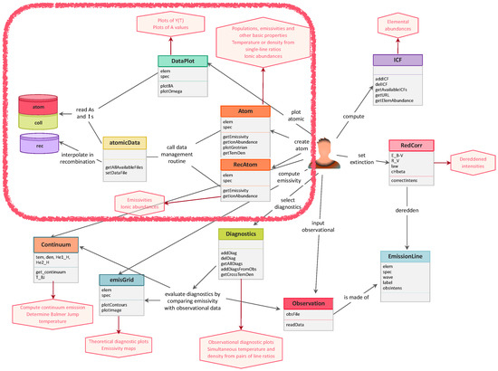
Figure 1.
Outline of the PyNeb object-oriented architecture showing its classes (name, some arguments, and methods) and output products. For atomic data assessment, we employ the classes and data within the red rectangle. The new Continuum class (added in Version 1.1.9) computes the nebular continuum (considering two-photon, free–free, and free–bound emission processes) and the electron temperature associated with the Balmer or Paschen jumps.
3. PyNeb Atomic Database
3.1. Data File Format
Earlier versions of PyNeb relied on data files structured under the FITS format [18,19] to comply with the IRAF6 Nebular package. These FITS files are still included in the current distribution, but are no longer used as default. Since 2014, a new ASCII format was adopted to allow the user easy access to the raw data and the addition of new data if needed. The old FITS files have been transcribed to this ASCII format, and new data are now incorporated in PyNeb only abiding this prescription. This format is close to that of the stout [14] database of the cloudy photoionization code, PyNeb being able to write its atomic data in stout format, but not always able to read from it (especially when different electron temperature grids are used in a single file). All the files holding the atomic data are downloaded and saved on the user’s disk when installing PyNeb; they can also be accessed from the GitHub repository under the pyneb/atomic_data directory.
3.2. Energy Levels
A frequent issue when dealing with complex ions (e.g., Fe or Fe) is to be able to compare the atomic parameters corresponding to the same transition, which requires a unique list of energy levels. We have therefore chosen to download the energy levels from the NIST Atomic Spectra Database7 and to sort them in increasing energy order. This may not always correspond to the list of separate multiplets (see, for instance, [20]) and involves the occasional data reordering to comply with the NIST energy-level order. The user can access the NIST energy levels with the function (for O, say):
pn.getLevelsNIST(’O3’)
3.3. Recombination Spectra for H and He
Recombination emissivities are read from the x_rec_ref.ext files, where x represents the ion and ref the source reference acronym. The ext extension may be either func or hdf5; for the former, a numerical function is used as in [21]. The data are read by the RecAtom class and interpolated in density and temperature. Recently, recombination data for the heavier ions of C, O, N, and Ne have also been incorporated into the PyNeb atomic database. For O, the recombination data table from [22] is split into infrared and optical–ultraviolet lines, and the A, B, and C cases are stored in separate files.
3.4. Collisional Spectra
For collisional spectra, PyNeb creates an -level atom model characterized by the atomic data read at runtime from the flat ASCII files _atom_ref.dat and _coll_ref.dat, where represents the ion (e.g., “o_iii” for O) and ref the source reference acronym. Transition probabilities (s) are different from zero only for , so the data are ordered in a rectangular matrix with zeroes along and above the main diagonal. The atom files contain the following items:
- Transition probabilities.
- Information about the corresponding ion.
- The data source reference.
The x_coll_ref.dat file contains the effective collision strengths (ECS) , which are functions of the electron temperature (i.e., a collective property of the electron distribution) obtained by averaging the energy-dependent collision strengths over a Maxwellian distribution of electron kinetic energies.
The ECS are usually published in tabular form for a handful of temperatures and must be interpolated to get the at the desired value. Such a table is included in the data file, and since for each transition , the upper level , there is a whole one-dimensional vector array of collision strengths with one element for each tabulated temperature value; that is, the complete set for an atom is a three-dimensional array that prevents confusing the data in the matrix with the transition probabilities (each transition is presented instead in a line). The temperature can be in Kelvin, log10(K), or K/10,000 depending on the particular dataset. The are interpolated linearly between the values at two contiguous temperatures; a keyword can be used to invoke an alternative interpolation method depending on what is available from the interpolate.interp1d function of the scipy library (e.g., “quadratic” or “cubic”). The interpolation method has some second-order influence on the resulting ECS, and thus on the emissivities.
The coll files contain the following quantities:
- Electron-temperature values used for the grid.
- ECS at the corresponding temperatures.
- Information about the corresponding ion (and the unit used for the electron temperature).
- Data source reference.
4. Data from CHIANTI
PyNeb can read the atomic data from the chianti8 package (Versions 7, 8, and 9, the latter the latest release; see [12,13]). The user needs the chianti database installed beforehand on their computer and the XUVTOP environment variable pointing to the corresponding directory. The chianti data (namely, level energies E, transition probabilities A, and ECS ) can be accessed using commands based on Chiantipy routines included in the PyNeb package (for O at 10,000 K, say):
- pn.utils.pn_chianti.Chianti_getA(’o_3’)
- pn.utils.pn_chianti.Chianti_getOmega(’o_3’, tem = 1e4)
The correspondence between the NIST and chianti level orders is obtained with the command:
- pn.utils.pn_chianti.get_levs_order(’O3’, NLevels = 9)
- -> {0: 0, 1: 1, 2: 2, 3: 3, 4: 4, 5: 5, 6: 8, 7: 6, 8: 7}
where the first number is the NIST index and the second the corresponding chianti index. We can see that Levels 7, 8, and 9 are not in the same order in both databases.
In chianti, the effective collision strength is mapped onto a finite temperature interval with the scaling relations of [23] and represented with a spline of five or more points. This ensures that a value can be obtained at any temperature . From Version 8, the mapping onto the scaled temperature interval is still used, but the stored points now correspond to the original data replacing the spline fits by interpolation. However, this only applies to new data; for the data already in the database, the 5-, 7-, or 9-point spline fits are still used [24]; e.g., a 5-point spline for O. Although this concise representation may not always be accurate, e.g., at low temperatures [24], it has endured and has been extended to neutral atoms and molecules [25]. In PyNeb, the original data are used. The extrapolation to low and high temperatures is performed by reporting the lowest and highest value, respectively. The user can avoid extrapolation by adding noExtrapolation = True when instantiating the Atom object; in this case, NaN values are returned for temperatures outside of the original range.
5. Atomic Data File Management
Within the scope of PyNeb in atomic data assessment, we go over the perhaps unfamiliar but core concept of the atomic data dictionary and its default value, the latter being the result of data selection procedures we are hereby trying to refine. We explain how to list the default and other dictionaries, the dataset labels, and respective bibliographic references and how to construct bespoke dictionaries to devise data comparisons.
5.1. Atomic Data Files
The collection of data files for the different ions used in a calculation is organized in a dictionary (in the Python sense); i.e., a data structure with one or more entries such that each entry has a uniquely defined key and value. An atomic data dictionary is identified by a label, which can be either predefined (i.e., built-in) or provided by the user; the keys are the ions, and the values specify the atomic data. More precisely, each value is itself a dictionary with three possible keys, “atom”, “coll”, or “rec”, whose respective values are the names of the atomic, collisional, or recombination data files.
The default dictionary of the current atomic database is obtained with the command:
- pn.atomicData.defaultDict
At present, it matches ’PYNEB_20_01’, but it will change as new atomic data are published or our criteria for selecting datasets evolves. The list of all the built-in atomic data labels is obtained with:
pn.atomicData.getAllPredefinedDict()
At the time of writing, 11 such dictionaries exist: ’IRAF_09_orig’, ’IRAF_09’, ’PYNEB_13_01’, ’PYNEB_14_01’, ’PYNEB_14_02’, ’PYNEB_14_03’, ’PYNEB_16_01’, ’PYNEB_17_01’, ’PYNEB_17_02’, ’PYNEB_18_01’, and ’PYNEB_20_01’. For the dictionary ’PYNEB_14_01’ and earlier, old FITS files are used, and a special command must be run before using them: pn.atomicData.includeFitsPath(). The old dictionaries are kept in PyNeb to guarantee backward compatibility, but users are strongly urged to use the default and to quote the PyNeb version in publication. As an example, the entry corresponding to the current O data is:
- pn.atomicData.getDataFile(atom = ’O3’)
- ’o_iii_atom_FFT04-SZ00.dat’,
- ’o_iii_coll_SSB14.dat’,
- ’o_iii_rec_P91.func’
If no value (or None) is specified for the atom keyword, the list of the data files for all the ions of the current configuration is returned as a dictionary.
The bibliographic references of the atomic data in the default dictionary are displayed with:
- pn.atomicData.printAllSources()
The bibliographic references of the atomic data used in a given dictionary labeled “label” (default or other) can be displayed by entering:
- pn.atomicData.printAllSources(predef = ’PYNEB_16_01’)
The bibliographic references of the atomic data used for just a subset of ions (e.g., O ii, O iii, and S ii) can be shown with:
- pn.atomicData.printAllSources(at_set = [’O2’, ’O3’, ’S2’])
5.2. Changing an Individual Data File or the Whole Dataset
The data available for a given ion (e.g., O iii) can be displayed by entering:
- pn.atomicData.getAllAvailableFiles(’O3’)
- [’* o_iii_atom_FFT04-SZ00.dat’,
- ’* o_iii_coll_SSB14.dat’,
- ’* o_iii_rec_P91.func’,
- ’o_iii_atom.chianti’,
- ’o_iii_atom_FFT04.dat’,
- ’o_iii_atom_GMZ97-WFD96.dat’,
- ’o_iii_atom_SZ00-WFD96.dat’,
- ’o_iii_atom_TFF01.dat’,
- ’o_iii_atom_TZ17.dat’,
- ’o_iii_coll.chianti’,
- ’o_iii_coll_AK99.dat’,
- ’o_iii_coll_LB94.dat’,
- ’o_iii_coll_MBZ20.dat’,
- ’o_iii_coll_Pal12-AK99.dat’,
- ’o_iii_coll_TZ17.dat’]
The data used to currently instantiate the Atom and RecAtom objects are identified with a leading asterisk (*). The current file selection for a given ion can be modified, for example, with the commands:
- pn.atomicData.setDataFile(’o_iii_atom_TZ17.dat’)
- pn.atomicData.setDataFile(’o_iii_coll_TZ17.dat’)
The next instantiating of an Atom object for O will use these data files. It is then simple to instantiate different Atom objects for the same ion with different atomic data to compare, for example, emissivities.
5.3. Deprecated Data
It may happen that at some point in the history of PyNeb, some atomic data files are removed from the default directory where all the data are stored. This mainly occurs if the same data are defined in another file that takes better into account the original source of the atomic data; in this case, the compilation is not used anymore (e.g., the data that used to be in the s_iii_atom_PKW09.dat file is now in the s_iii_atom_FFTI06.dat file to cite the original paper). When this occurs, the obsolete file is sent to the deprecated directory to ensure backward compatibility. If the user still prefers to have access to the data in this directory, the command pn.atomicData.includeDeprecatedPath() is needed before permuting the default data file with the deprecated one. Removing deprecated files from the accessible path is performed with pn.atomicData.removeDeprecatedPath().
5.4. List of All the Data Used in a Script
Each time an Atom or a RecAtom object is instantiated, the data files used are stored in a dictionary held by the atomicData object. After a script is run using PyNeb, the list of all the files can be obtained using the pn.atomicData.usedFiles command. This helps the user cite the atomic data papers properly.
6. Continuum Class: Balmer and Paschen Jumps to Determine the Electron Temperature
Continuum is a new class in PyNeb (see Figure 1) devised to obtain alternative estimates of the electron temperature. This is an important development as the temperatures derived from line diagnostics strongly depend on the basic atomic database, whose accuracy is often questioned in the literature (e.g., [26]).
6.1. Nebular Continuum
The nebular continuum due to the following processes,
- Free–bound emission from H, He, and He [27],
- Free–free emission by H, He, and He [28],
- Two-photon decay from 2S of H [17],
can be estimated with PyNeb. The prescription to obtain the continuum is: wavelength range; electron temperature and density; and the He/H and He/H ionic abundances. The continuum is given in erg s cmÅ or in Å when normalized to an H i line. The commands:
- C = pn.core.continuum.Continuum()
- C.get_continuum(tem = 1e4, den = 1e2, He1_H = 0.12, He2_H = 0.01,
- wl = np.linspace(3500, 3900, 100), HI_label = ’11_2’)
give an example on how to compute the continuum normalized to H i 3770 Å for: K; cm; ; and in the wavelength range 3500–3900 Å. The result of this example is plotted in Figure 2. To get the continuum with no normalization, HI_label must be defined as None.
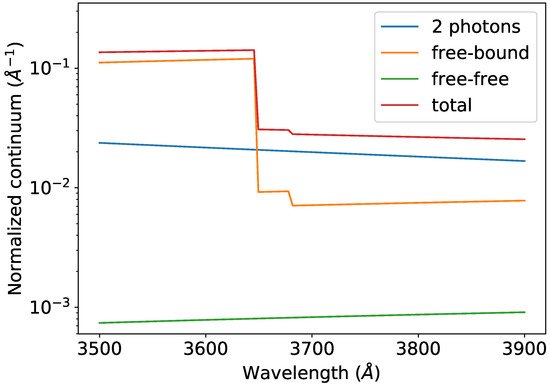
Figure 2.
Nebular continuum normalized to H i 3770 Å. The data are obtained with the get_continuum function of the Continuum class for K, cm, He/H, and He/H.
6.2. Balmer and Paschen Jump Temperatures
The electronic temperature from the Balmer (or Paschen) jump is determined by minimizing the difference between the theoretical nebular continuum (described in Section 6.1) and the observed flux before and after the jump. The optimization is based on the Richard Brent algorithm for root-finding [29] using scipy.optimize.brentq.
The temperature determination requires: the difference of the observed flux (in Å) before and after the jump normalized to a H i line; the corresponding wavelengths (predefined at 3643 and 3861 Å); the electron density; and the He/H and He/H ionic abundances. The following example uses the data for the planetary nebula M 1-42 [30] normalized to H i 3770 Å and to H:
- C.T_BJ(BJ_HI = 0.23, den = 1500, He1_H = 0.139, He2_H = 0.009,wl_bbj = 3643,
- wl_abj = 3861, HI_label = ’11_2’, T_min = 500.0, T_max = 30000.0)
- 3748.803973930705
- C.T_BJ(BJ_HI = 8.56e-3, den = 1500, He1_H = 0.139, He2_H = 0.009,
- wl_bbj = 3643, wl_abj = 3861, HI_label=’4_2’, T_min = 500.0, T_max = 30,000.0)
- 3910.6448636964446
The contributions from the stellar continuum and dust emission are not considered in the temperature determination, although they can contribute to the observed flux.
7. Atomic Data Assessment
A paradigmatic example of using PyNeb for atomic data assessment is [31], who analyzed the size of the systematic uncertainties when using 52 different sets of transition probabilities and collision strengths to calculate the physical conditions and total abundances of O, N, S, Ne, Cl, and Ar for a sample of planetary nebulae and H ii regions. These authors found that at low densities, the scatter in the abundance ratios was lower than 0.1–0.2 dex9, but for densities cm, it can be larger than 0.6–0.8 dex for several abundance ratios such as O/H and N/O. A narrower scatter was obtained by discarding questionable atomic data, but a revision of the atomic data behind important density diagnostics was recommended: the radiative transition probabilities (A-values) of O ii, S ii, Cl iii, and Ar iv, as well as the effective collision strengths for the latter.
In the last few years, there has been growing interest in determining chemical abundances in ionized nebulae for the heavier elements nucleosynthesized by slow-neutron capture (the s-process). Encouraged by several detections of s-process faint emission lines in planetary nebulae, several groups have been computing the required atomic data; e.g., Rb iv [32]; Se iii and Kr vi [33]; and Te iii and Br v [34]. The synergy between observations, atomic data calculations, and numerical modeling (needed to determine ICF) has significantly boosted this field. All these atomic datasets for neutron-capture elements (energy levels, transition probabilities, and collision strengths) have been incorporated in PyNeb, allowing, for the first time, total abundance estimates for Kr and Se by using the complete sets of ICF developed for these elements by [33,34] using a private ad hoc version of cloudy.
The DataPlot class has several methods to plot the atomic datasets, which can be used to bring out the data scatter and questionable outliers. For instance, the commands:
- dp_O3=pn.DataPlot(’O’,3,NLevels = 5)
- dp_O3.plotAllA(figsize = (10,8))
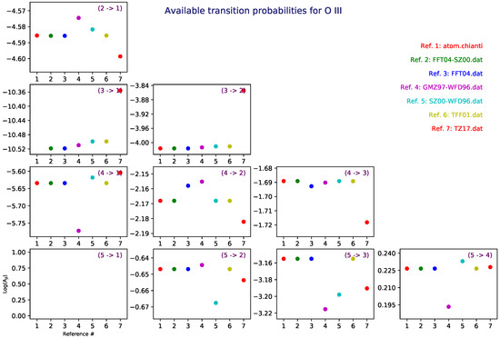
Figure 3.
O iii A-value diagram obtained with the plotAllA method of the DataPlot class.
To further illustrate the possibilities of the PyNeb analysis tools in atomic data assessment, we discuss in the next sections two relevant study cases.
7.1. A-Values for N- and P-Like Ions
We address here one of the atomic data queries raised by [31]: the radiative rates for the N-like (O ii and Ne iv) and P-like (S ii, Cl iii, and Ar iv) systems, which are widely used to devise nebular density diagnostics. These are ionic species with ground configuration ( for N-like and for P-like), the line ratio of interest being the doublet. Figure 4 shows the energy-level structure and radiative transitions of O ii plotted with the PyNeb commands:
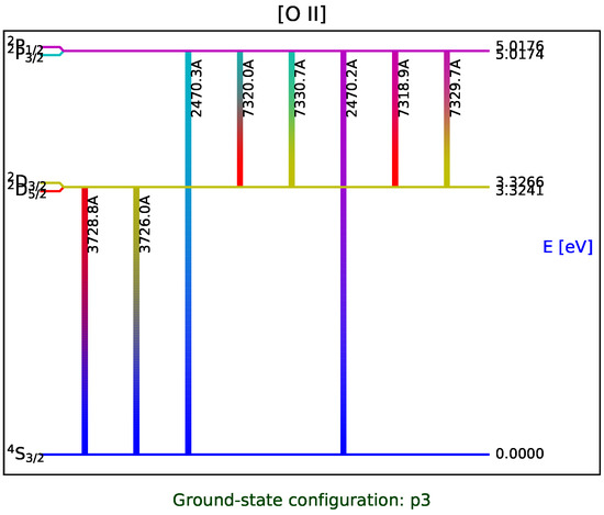
Figure 4.
O ii Grotrian diagram obtained with the plotGrotrian method of the Atom class.
- O2 = pn.Atom(’O’,2)
- O2.plotGrotrian()
in particular the 3729/3726 density-sensitive doublet.
In the context of nebular physics, the accuracy of the A-values for O ii and S ii have been previously discussed [4,5,35]. For data assessment purposes, the A-value ratio:
was therein prescribed to provide a useful observational benchmark since:
that is, at high densities, the line intensity ratio depends mostly on the doublet A-values, and therefore physically:
Using the getEmissivity method, we plot in Figure 5 the percentage difference of the emissivity ratio in N-like ions at K computed with A-values from the GFF84 [36], Z87 [37], WFD96 [38], and FFT04 [39] datasets relative to Z82 [40]. All these calculations have been performed with a relativistic Breit–Pauli Hamiltonian; they account for electron correlation effects, and some include corrections to the magnetic dipole operator and level energy separations to increase accuracy. Significant discrepancies due to the A-value choice begin to appear at electron densities cm, and most grow with density until is reached. For both O ii and Ne iv, the emissivity-ratio uncertainties from the radiative data are no larger than 25% along the entire density range.
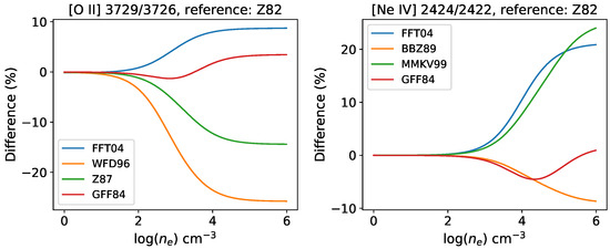
Figure 5.
Comparison of density-sensitive emissivity ratio of N-like ions computed at K with different A-value datasets relative to Z82. Left panel: [O ii] . Right panel: [Ne iv] . Source references for the A-value datasets are given in Table 1.
A further measure of A-value accuracy can be carried out in terms of the A-value ratio and a benchmark with the observed line ratios from the high-density NGC 7027 planetary nebula [41] as listed in Table 1. The overall agreement between the theoretical ratios is around the 15% level. Interestingly, the more recent calculations (CQL07 [42], HGZJYL14 [43], and HLZSZ18 [44]) have focused to constrain using a fully relativistic multi-configuration Dirac–Fock (MCDF) method with convergent configuration-interaction expansions, which includes the Breit interaction and QED effects. Although the from these calculations is within the general scatter, the absolute values from these calculations are somewhat larger than previous estimates.

Table 1.
Theoretical A-values (s) for the doublet within the ground configuration of N-like O ii and Ne iv. The ratio is also given for comparison with the line intensity ratio observed in the dense NGC 7027 planetary nebula.
It may be seen in Table 1 that the observed [O ii] line ratio is in good agreement with the theoretical values, while in Ne iv, it is noticeably higher, implying that the high-density regime for this latter diagnostic has not been reached in NGC 7027, and it can therefore be used to obtain the electron density. We deduce an electron density of cm at K using the Z82, GFF84, BBZ89, MMKV99, and FFT04 datasets, giving an estimate of the impact of the atomic data scatter on the density diagnostic, namely 0.1 dex. Since one of the main objectives of the present work is to select default atomic datasets in PyNeb, we singled out Z82 and GFF84 for both O ii and Ne iv after much pondering to ensure line ratio diagnostics within 10%. For this purpose, we applied the following selection criteria:
- Datasets must contain all the transitions within the ground configuration with at least .
- For consistency, datasets considering isoelectronic sequences are preferred to those focusing on single species.
- Wavelength adjusted A-values computed with correct transition operators (e.g., magnetic dipole) have priority.
- Emissivity ratios must lie within a 10% scatter along the isoelectronic sequence.
- The dataset must comply with the condition of Equation (10), and must lie within a 10% theoretical scatter.
- A selected dataset must be validated with data computed independently with a different numerical method.
Among the Z82, GFF84, BBZ89, MMKV99, and FFT04 datasets, only the first two comply with these selection criteria.
We repeat this data assessment procedure with the ionic species of the P isoelectronic sequence of nebular interest, namely S ii, Cl iii, and Ar iv. In Figure 6, we plot the percentage difference of the emissivity ratio computed with the FFG86 [47], KHOC93 [48], Fal99 [49], IFF05 [50], FFT06 [51], TZ10 [52], KKFBL14 [53], and RGJ19 [54] A-value datasets relative to MZ82 [55]. Similar to the N-like ions, the overall agreement is around the 25% level, but if we exclude the three datasets FFG86, TZ10, and KKFBL14 in S ii (see Figure 6 left panel), the agreement is better than 10%. The emissivity ratio discrepancies from the fully relativistic (MCDF) Fal99 and RGJ19 datasets relative to MZ82 are puzzling and not explained in [54]: for the former, they increase with atomic number Z up to 15% in Ar iv, while in the latter they remain within 5% throughout the isoelectronic sequence (see all panels of Figure 6).
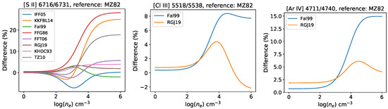
Figure 6.
Comparison of the density-sensitive emissivity ratio of P-like ions computed at K with different A-value datasets relative to MZ82. Left panel: [S ii] . Center panel: [Cl iii] . Right panel: [Ar iv] . Source references for the A-value datasets are given in Table 2.
In Table 2, we compare the theoretical for the three ions with the line ratios observed in NGC 7027. If we again exclude FFG86, TZ10, and KKFBL14, we find excellent agreement in S ii. Assuming the A-value scatter, the predicted electron densities for Cl iii and Ar iv are cm and cm, respectively; i.e., within 0.1 dex. From these comparisons and following our selection criteria, we confidently single out the recent RGJ19 dataset [54] as the PyNeb default to ensure a line ratio with an uncertainty from the radiative data better than 10%. The PYNEB_20_01 dictionary with the PyNeb default values adopts these datasets.
Table 2.
Theoretical A-values (s) for the doublet within the ground configuration of P-like S ii, Cl iii, and Ar iv. The ratio is also given for comparison with the line-intensity ratio observed in the dense NGC 7027 planetary nebula.
7.2. Effective Collision Strengths for C-Like Ions
The present evaluation of the ECS for ions of the carbon isoelectronic sequence is motivated on the one hand by the leading role of their temperature diagnostics in nebular modeling and on the other by the worrisome discrepancies resulting when using an extensive ECS dataset for C-like ions () recently published (MBZ20 [56]). In Figure 7, we plot the percentage difference of the [N ii] 5755/6584 and [O iii] 4363/5007 emissivity ratios using the ECS from the LB94 [57], HB04 [58], and MBZ20 datasets relative to T11 [59] (default) for the former and from LB94, AK99 [60], Pal12-AK99 [61], TZ17 [62], and MBZ20 relative to SSB14 [63] (default) for the latter. While the accord of LB94, AK99, and TZ17 with SSB14 for O iii and of LB94 and HB04 with T11 for N ii is well within 10% for both species, MBZ20 shows large discrepancies: as high as −50% in O iii and +30% in N ii. As also shown in Figure 7 (left panel), the emissivity ratio resulting from the Pal12-AK99 ECS for O iii is ∼25% higher and is caused by their neglecting the 2p free channels in the close-coupling expansion of the ion–electron system that leads to an energy downshift of the broad 2p resonance [63].
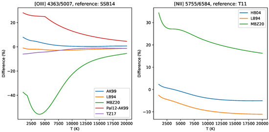
Figure 7.
Comparison of the temperature-sensitive emissivity ratios of [O iii] 4363/5007 (left panel) and [N ii] 5755/6584 (right panel) computed at cm. For [O iii], we compare the ratios obtained when using the SSB14 default ECS [63] with other datasets; for [N ii], the default ECS are T11 [59]. Data provenance is: LB94 [57]; AK99 [60]; HB04 [58]; Pal12 [61]; TZ17 [62]; and MBZ20 [56].
The large discrepancies in the emissivity ratios originating from the MBZ20 ECS are of concern and demand further analysis. For instance, in Figure 8, we plot the temperature differences when using MBZ20 relative to the default ECS datasets: for a set of temperatures and densities, we compute the diagnostic line ratios [N ii] 5755/6584 and [O iii] 4363/5007, and from them, we compute back the electron temperature determined using MBZ20. (N ii) is underestimated by as much as 1.6 kK at 14 kK, while (O iii) is overestimated by 0.8 kK. This temperature divergence may have a significant impact on the ionic abundances since (N ii) is used in nebular models for the singly ionized species (N, O, and S), while (O iii) is used for O, Ar, and S.
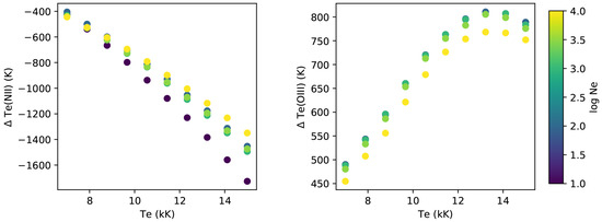
Figure 8.
Temperature differences caused by using the MBZ20 ECS relative to the PyNeb defaults. Left panel: (N ii). Right panel: (O iii).
In Figure 9, we show the resulting abundance logarithmic differences: we compute the emissivities of the emission lines with the PyNeb default atomic data and then use them to compute back the ionic abundances with MBZ20. They are obtained at five electron densities (10, 100, 1000, 3000, and 10,000 cm) from the following emission lines: [N ii] 6584; [O ii] 3726 + 29; [O iii] 5007; [Ar iii] 7135; [S ii] 6716 + 31; and [S iii] 6312 and 9069. The differences (positive and negative) can be as large as 0.3 dex when considering low or high ionization species. Depending on the global ionization of the nebula, the total abundance may be underestimated (high-ionization nebulae) or overestimated (low-ionization nebulae) depending on the dominant ionic stage of each element. For medium-ionization nebulae, the net result may be a cancellation between both effects, leading to the same elemental abundances.
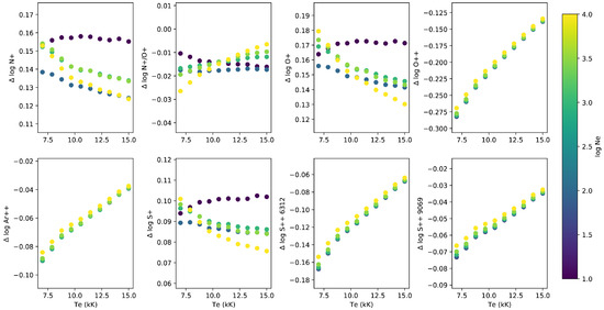
Figure 9.
Abundance logarithmic differences for several ions caused by using the MBZ20 ECS relative to the PyNeb defaults.
The DataPlot class offers a series of useful methods to plot the atomic data, which can be used to revise the MBZ20 datasets for O iii and N ii:
- dp_O3=pn.DataPlot(’O’,3,NLevels = 5)
- dp_O3.plotOmega(figsize = (10,8))
- dp_N2=pn.DataPlot(’N’,2,NLevels = 5)
- dp_N2.plotOmega(figsize = (10,8))
the resulting plots being shown in Figure 10 and Figure 11. For O iii, it may be seen that the , , and ECS by MBZ20 corresponding to the transitions are considerably larger in the temperature region of interest ( kK). On the other hand, the situation in N ii for these transitions is the inverse: the MBZ20 ECS are now lower. The from different datasets for both O iii and N ii also displays incongruent behaviors. However, we underline that MBZ20 is the only dataset offering ECS for temperatures K.
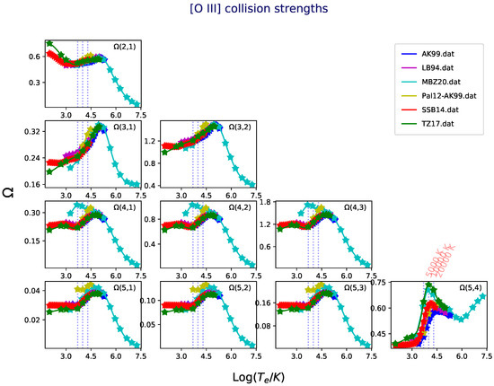
Figure 10.
Available ECS for O iii in PyNeb plotted with the plotOmega method of the DataPLot class. Note that “collision strengths” and in this figure stand for temperature-dependent ECS.
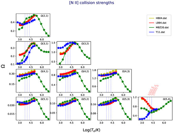
Figure 11.
Available ECS for N ii in PyNeb plotted with the plotOmega method of the DataPLot class. Note that “collision strengths” and in this figure stand for temperature-dependent ECS.
Figure 10 and Figure 11 illustrate a recurrent problem in nebular modeling when dealing with ECS tabulations. The temperature end-points and mesh intervals in each dataset vary, and they must be somehow interpolated. In chianti, the ECS are sometimes represented by five, six, or seven points, two of which are assigned to and ; thus, in real terms, the finite temperature range is reduced to three, four, or five point spline fits, which may result in further inaccuracies.
In Figure 12 (left panel), we plot the collision strength for the [O iii] transition computed by MBZ20 and SSB14, which is dominated in the near-threshold region by a broad peak. In SSB14, this peak is located at ≈0.29 Ryd, while in MBZ20, it downshifts to ≈0.22 Ryd, causing the ECS enhancement shown in Figure 10. As discussed by [62], there is an experimental position for this peak at 0.294 Ryd [64]; thus, the downshifted resonance position in MBZ20 is inaccurate. This peak is mainly caused by an array of resonances with configuration 2s2p3s, and their atomic structure does not represent these states adequately. Moreover, the resonance structure in the two curves in the energy interval Ryd is also different (see Figure 12, left panel).
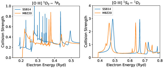
Figure 12.
Collision strength for the transitions [O iii] (left panel) and (right panel) computed by SSB14 and MBZ20.
The ECS in Figure 10 corresponds to the [O iii] transition, and the data by SSB14 and MBZ20 are also found to be discrepant in the temperature region of interest. As shown in Figure 12 (right panel), this discord is again caused by resonance positions, in this case the near-threshold 2p resonance that in MBZ20 is around 0.02 Ryd lower. Although this downshift is relatively smaller, the resonance is closer to the threshold, making the ECS sensitive at low temperatures. Moreover, it is also seen in Figure 10 that the by MBZ20 and TZ17 are in agreement. We therefore predict that the position of this resonance in TZ17 is also lower than in SSB14, and we would then be of the opinion that the latter dataset is the most accurate and, therefore, the PyNeb default. Similar discrepancies are observed in the in N ii (see Figure 11), which were discussed in [5] and need further evaluation.
8. Discussion and Conclusions
In the context of nebular modeling, we made use of the atomic data assessment capabilities of PyNeb to revise the accuracy of the A-values for transitions within the ground configuration of the N- and P-like ions as suggested by [31] and the ECS for C-like species motivated by the recent publication of an extensive dataset [56]. For atomic data evaluation, PyNeb offers two coveted features: a fairly complete historical database of radiative and collisional parameters and a handy series of class methods to compare plasma diagnostics and abundances using the different atomic datasets, which enable direct uncertainty estimates in parameter space. As a result, we have been able to select for these isoelectronic sequences the reference datasets to become the PyNeb defaults.
The magnitude and scatter of the lifetimes of the two S ii 3s3p levels have been extensively reviewed recently to propose a viable measurement scheme to improve their accuracy to better than 10% [65]. It was mentioned therein that a 10% lifetime uncertainty would lead to a 50% emissivity ratio uncertainty and that the current theoretical scatter is larger than 10%. Due to inherent experimental difficulties to measure the very long lifetimes of the levels (∼1 h), the more feasible task of measuring the lifetimes of the levels (a few seconds) was developed. In the present work, we showed that theory can do better than 50%: for both the N- and P-like ions of nebular interest, the emissivity ratio uncertainties despite the A-value scatter are within 25%. Furthermore, by means of the high-density benchmark with the observed line ratios (i.e., from the NGC 7027 planetary nebula), we can discard A-value datasets to reduce the emissivity ratio uncertainty to the 10% level with some degree of assurance. However, we notice that, in spite of accurate ratios, the absolute A-values in some datasets are somewhat larger, particularly those for [O ii] recently computed with the MCDF method [42,43,44]. This type of discrepancy can only be resolved by measurement, although we remain skeptical in light of the long-standing discord between theory and experiment regarding the Fe xvii 3C/3D f-value ratio [66].
Regarding the recent MBZ20 ECS for the carbon sequence [56], we demonstrated that this dataset leads to large discrepancies in the emissivity ratios of both N ii and O iii and should therefore not be used in the electron temperature range kK. As shown in Figure 12, the broad peak at ≈0.29 Ryd in the O iii collision strength by SSB14 [63] (default) is downshifted in MBZ20 to ≈0.22 Ryd, in disagreement with an experimental benchmark of 0.294 Ryd [62,64]. The origin of this discrepancy may be found in the large O iii atomic model (590 fine-structure levels from 24 configurations including orbitals with principal quantum number ) of MBZ20, which has been optimized specifically to provide ECS at high temperatures. They adjusted the -dependent scaling parameters in a systematic way without manual re-adjustment to avoid introducing arbitrary changes across the isoelectronic sequence. This strategy leads to poor atomic structure for low-charge ions such as O iii and, thus, less accurate collision data at low temperatures. At high temperatures, the resonance effect is reduced, so their data should be more accurate (Mao Junjie, private communication). As a result, we can conclude that the uncertainty level in the [N ii] 5755/6584 emissivity ratios using ECS from LB94, HB04, and T11 and in [O iii] 4363/5007 from LB94, AK99, SSB14, and TZ17 is within 10%. This outcome is a good example that the latest and largest atomic calculation is not necessarily the most accurate and should therefore be carefully examined, as we showed here, before data are included in plasma models. This last point has also been stressed in the context of the long-standing discrepancies in the ECS computed for Be-like ions by independent R-matrix methods [67].
After providing and applying atomic data in nebular modeling for almost five decades, we are amazed at not being able to guarantee an acceptable level of accuracy. However, the present work contributes to clarifying that computations for low- and high-energy regimes cannot be treated simultaneously with the same level of accuracy, a fact that must be taken into account in atomic database maintenance. We tend to agree with [65] that we have a laboratory astrophysics problem in hand with no foreseeable solution due to the endemic difficulties in computing, measuring, and evaluating the data products. As proposed in [16], open and fluid user–provider interactions and early data curation schemes in the research cycle are perhaps the best we can do.
As future work within the present initiative, we intend to revise and complete the atomic data for the lowly ionized species of the iron-group elements, for which there are non-conclusive accuracy evaluations. We would finally like to mention that, in reference to data-curation strategies, a historical atomic database as kept in PyNeb is a welcome step in data preservation, and the choice of a flat ASCII format rather than FITS to facilitate longevity and user interaction must be seriously considered in database design.
Author Contributions
C.M. (Christophe Morisset) and C.M. (Claudio Mendoza) conceptualized and coordinated the full paper. Investigation, methodology, analysis, and validation, J.G.-R., M.B., and V.G.-L.; software, V.L., J.G.-R., and C.M. (Christophe Morisset); writing, the original draft preparation, V.L., J.G.-R., C.M. (Christophe Morisset), and C.M. (Claudio Mendoza); writing, review and editing, J.G.-R., M.B., C.M. (Christophe Morisset), and C.M. (Claudio Mendoza); visualization, V.L., V.G.-L., C.M. (Christophe Morisset), and C.M. (Claudio Mendoza); ancillary calculations, M.B. All authors read and agreed to the published version of the manuscript.
Funding
C.M. (Christophe Morisset) and V.G.-L. acknowledge support from the Mexican CONACyT-CB2015-254132 and UNAM-DGAPA-PAPIIT-101220 projects. C.M. (Claudio Mendoza) is grateful for financial support from the NASA Astrophysics Research and Analysis Program (Grants 12-APRA12-0070 and 80NSSC17K0345). J.G.-R. acknowledges support from an Advanced Fellowship from the Severo Ochoa excellence program (SEV-2015-0548) and from the State Research Agency (AEI) of the Spanish Ministry of Science, Innovation and Universities (MCIU) and the European Regional Development Fund (FEDER) under Grant AYA2017-83383-P. J.G.-R. also acknowledges support under Grant P/308614 financed by funds transferred from the Spanish Ministry of Science, Innovation and Universities, charged to the General State Budgets and with funds transferred from the General Budgets of the Autonomous Community of the Canary Islands by the MCIU.
Acknowledgments
We are grateful to Mao Junjie (Strathclyde University, U.K.) for giving us access to the raw collision strengths of [56] and for helpful and clarifying discussions and to Elmar Träbert (Ruhr-Universität Bochum, Germany) for enlightening comments on measuring the immeasurable. We are indebted to Grażyna Stasińska (Observatoire de Paris, France) for regular suggestions to improve PyNeb in the last decade, especially during the preparation of the NEBULATOM workshops. We thank these three colleagues for critically reading the manuscript and providing useful comments and addenda that led to its improvement. This paper have been written using the Overleaf web service.
Conflicts of Interest
The authors declare no conflict of interest.
Abbreviations
The following abbreviations are used in this manuscript:
| FITS | Flexible Image Transport System |
| NIST | National Institute of Standards and Technology |
| QED | Quantum electrodynamics |
References
- Luridiana, V.; Morisset, C.; Shaw, R.A. PyNeb: A new software for the analysis of emission lines. In IAU Symposium; Cambridge Univ. Press: Cambridge, UK, 2012; Volume 283, pp. 422–423. [Google Scholar] [CrossRef]
- Luridiana, V.; Morisset, C.; Shaw, R.A. PyNeb: A new tool for analyzing emission lines. I. Code description and validation of results. Astron. Astrophys. 2015, 573, A42. [Google Scholar] [CrossRef]
- Peimbert, M.; Peimbert, A.; Delgado-Inglada, G. Nebular Spectroscopy: A Guide on H II Regions and Planetary Nebulae. Publ. Astron. Soc. Pac. 2017, 129, 082001. [Google Scholar] [CrossRef]
- Stasińska, G.; Prantzos, N.; Meynet, G.; Simón-Díaz, S.; Chiappini, C.; Dessauges-Zavadsky, M.; Charbonnel, C.; Ludwig, H.G.; Mendoza, C.; Grevesse, N.; et al. Appendix A: The Atomic Physics of Oxygen; EAS Publications Series; Stasińska, G., Prantzos, N., Meynet, G., Simón-Díaz, S., Chiappini, C., Dessauges-Zavadsky, M., Charbonnel, C., Ludwig, H.G., Mendoza, C., Grevesse, N., et al., Eds.; EDP Sciences: Les Ulils, France, 2012; Volume 54, pp. 319–335. [Google Scholar] [CrossRef]
- Mendoza, C.; Bautista, M.A. Testing the Existence of Non-Maxwellian Electron Distributions in H II Regions after Assessing Atomic Data Accuracy. Astrophys. J. 2014, 785, 91. [Google Scholar] [CrossRef]
- Badnell, N.R.; Ferland, G.J.; Gorczyca, T.W.; Nikolić, D.; Wagle, G.A. Bootstrapping Dielectronic Recombination from Second-row Elements and the Orion Nebula. Astrophys. J. 2015, 804, 100. [Google Scholar] [CrossRef]
- Pradhan, A.K.; Nahar, S.N. Atomic Astrophysics and Spectroscopy; Cambridge University Press: Cambridge, UK, 2011. [Google Scholar]
- Luridiana, V.; García-Rojas, J.; Aggarwal, K.; Bautista, M.; Bergemann, M.; Delahaye, F.; del Zanna, G.; Ferland, G.; Lind, K.; Manchado, A.; et al. How to Make an Atomic Blog in Your Own Kitchen. Summary of the Workshop: Uncertainties in Atomic Data and How They Propagate in Chemical Abundances. arXiv 2011, arXiv:1110.1873. [Google Scholar]
- Luridiana, V.; García-Rojas, J. Report on the Tenerife Workshop on Uncertainties in Atomic Data and How They Propagate in Chemical Abundances; Cambridge University Press: Cambridge, UK, 2012; Volume 283, pp. 139–143. [Google Scholar] [CrossRef]
- Mendoza, C. Recent advances in atomic calculations and experiments of interest in the study of planetary nebulae. In Planetary Nebulae; Aller, L.H., Ed.; Reidel: Dordrecht, The Netherlands, 1983; Volume 103, pp. 143–172. [Google Scholar]
- Mendoza, C. Atomic Databases: Four of a Kind. Atoms 2020, 8, 30. [Google Scholar] [CrossRef]
- Dere, K.P.; Landi, E.; Mason, H.E.; Monsignori Fossi, B.C.; Young, P.R. CHIANTI—An atomic database for emission lines. Astrophys. J. 1997, 125, 149–173. [Google Scholar] [CrossRef]
- Dere, K.P.; Del Zanna, G.; Young, P.R.; Landi, E.; Sutherland, R.S. CHIANTI—An Atomic Database for Emission Lines. XV. Version 9, Improvements for the X-Ray Satellite Lines. Astrophys. J. Suppl. Ser. 2019, 241, 22. [Google Scholar] [CrossRef]
- Ferland, G.J.; Chatzikos, M.; Guzmán, F.; Lykins, M.L.; van Hoof, P.A.M.; Williams, R.J.R.; Abel, N.P.; Badnell, N.R.; Keenan, F.P.; Porter, R.L.; et al. The 2017 Release Cloudy. Rev. Mex. Astron. Astrofis. 2017, 53, 385–438. [Google Scholar]
- Bautista, M.A.; Kallman, T.R. The XSTAR Atomic Database. Astrophys. J. Suppl. Ser. 2001, 134, 139–149. [Google Scholar] [CrossRef]
- Mendoza, C.; Boswell, J.; Ajoku, D.; Bautista, M. AtomPy: An Open Atomic Data Curation Environment for Astrophysical Applications. Atoms 2014, 2, 123. [Google Scholar] [CrossRef]
- Osterbrock, D.E.; Ferland, G.J. Astrophysics of Gaseous Nebulae and Active Galactic Nuclei; University Science Books: Sausalito, CA, USA, 2006. [Google Scholar]
- Greisen, E.W. FITS: A Remarkable Achievement in Information Exchange. In Information Handling in Astronomy—Historical Vistas; Heck, A., Ed.; Astrophysics and Space Science Library; Kluwer Academic Publishers: Dordrecht, The Netherlands, 2003; Volume 285, p. 71. [Google Scholar] [CrossRef]
- Pence, W.D.; Chiappetti, L.; Page, C.G.; Shaw, R.A.; Stobie, E. Definition of the Flexible Image Transport System (FITS), version 3.0. Astron. Astrophys. 2010, 524, A42. [Google Scholar] [CrossRef]
- Zhang, H. Atomic data from the Iron Project. XVIII. Electron impact excitation collision strengths and rate coefficients for Fe III. Astron. Astrophys. Suppl. Ser. 1996, 119, 523–528. [Google Scholar] [CrossRef]
- Pequignot, D.; Petitjean, P.; Boisson, C. Total and effective radiative recombination coefficients. Astron. Astrophys. 1991, 251, 680–688. [Google Scholar]
- Storey, P.J.; Sochi, T.; Bastin, R. Recombination coefficients for O II lines in nebular conditions. Mon. Not. R. Astron. Soc. 2017, 470, 379–389. [Google Scholar] [CrossRef]
- Burgess, A.; Tully, J.A. On the analysis of collision strengths and rate coefficients. Astron. Astrophys. 1992, 254, 436–453. [Google Scholar]
- Del Zanna, G.; Dere, K.P.; Young, P.R.; Landi, E.; Mason, H.E. CHIANTI—An atomic database for emission lines. Version 8. Astron. Astrophys. 2015, 582, A56. [Google Scholar] [CrossRef]
- Summers, H.P.; Kato, T. Extension of the Burgess-Tully method to fit neutral atom and molecule cross-sections. Astron. Astrophys. Suppl. Ser. 2000, 144, 501–507. [Google Scholar] [CrossRef]
- Nicholls, D.C.; Dopita, M.A.; Sutherland, R.S.; Kewley, L.J.; Palay, E. Measuring Nebular Temperatures: The Effect of New Collision Strengths with Equilibrium and κ-distributed Electron Energies. Astrophys. J. Suppl. Ser. 2013, 207, 21. [Google Scholar] [CrossRef]
- Ercolano, B.; Storey, P.J. Theoretical calculations of the H I, He I and He II free-bound continuous emission spectra. Mon. Not. R. Astron. Soc. 2006, 372, 1875–1878. [Google Scholar] [CrossRef]
- Storey, P.J.; Hummer, D.G. Fast computer evaluation of radiative properties of hydrogenic systems. Comput. Phys. Commun. 1991, 66, 129–141. [Google Scholar] [CrossRef]
- Brent, R.P. Algorithms for Minimization without Derivatives; Dover Publications: Mineola, NY, USA, 2002. [Google Scholar]
- Liu, X.W.; Luo, S.G.; Barlow, M.J.; Danziger, I.J.; Storey, P.J. Chemical abundances of planetary nebulae from optical recombination lines—III. The Galactic bulge PN M 1–42 and M 2–36. Mon. Not. R. Astron. Soc. 2001, 327, 141–168. [Google Scholar] [CrossRef]
- Juan de Dios, L.; Rodríguez, M. The impact of atomic data selection on nebular abundance determinations. Mon. Not. R. Astron. Soc. 2017, 469, 1036–1053. [Google Scholar] [CrossRef]
- Sterling, N.C.; Dinerstein, H.L.; Kaplan, K.F.; Bautista, M.A. Discovery of Rubidium, Cadmium, and Germanium Emission Lines in the Near-infrared Spectra of Planetary Nebulae. Astrophys. J. 2016, 819, L9. [Google Scholar] [CrossRef]
- Sterling, N.C.; Madonna, S.; Butler, K.; García-Rojas, J.; Mashburn, A.L.; Morisset, C.; Luridiana, V.; Roederer, I.U. Identification of Near-infrared [Se III] and [Kr VI] Emission Lines in Planetary Nebulae. Astrophys. J. 2017, 840, 80. [Google Scholar] [CrossRef]
- Madonna, S.; Bautista, M.; Dinerstein, H.L.; Sterling, N.C.; García-Rojas, J.; Kaplan, K.F.; del Mar Rubio-Díez, M.; Castro-Rodríguez, N.; Garzón, F. Neutron-capture Elements in Planetary Nebulae: First Detections of Near-infrared [Te III] and [Br V] Emission Lines. Astrophys. J. 2018, 861, L8. [Google Scholar] [CrossRef]
- Stasińska, G.; Peña, M.; Bresolin, F.; Tsamis, Y.G. Planetary nebulae and H II regions in the spiral galaxy NGC 300. Clues on the evolution of abundance gradients and on AGB nucleosynthesis. Astron. Astrophys. 2013, 552, A12. [Google Scholar] [CrossRef]
- Godefroid, M.; Fischer, C.F. MCHF-BP fine-structure splittings and transition rates for the ground configuration in the nitrogen sequence. J. Phys. B Atom. Mol. Phys. 1984, 17, 681–692. [Google Scholar] [CrossRef]
- Zeippen, C.J. Improved radiative transition probabilities for O II forbidden lines. Astron. Astrophys. 1987, 173, 410–414. [Google Scholar]
- Wiese, W.L.; Fuhr, J.R.; Deters, T.M. Atomic Transition Probabilities of Carbon, Nitrogen, and Oxygen: A Critical Data Compilation. JPCRD, Monograph Np. 7; AIP: Washington, DC, USA, 1996. [Google Scholar]
- Froese Fischer, C.; Tachiev, G. Breit-Pauli energy levels, lifetimes, and transition probabilities for the beryllium-like to neon-like sequences. Atom. Data Nucl. Data Tables 2004, 87, 1–184. [Google Scholar] [CrossRef]
- Zeippen, C.J. Transition probabilities for forbidden lines in the 2p3 configuration. Mon. Not. R. Astron. Soc. 1982, 198, 111–125. [Google Scholar] [CrossRef][Green Version]
- Zhang, Y.; Liu, X.W.; Luo, S.G.; Péquignot, D.; Barlow, M.J. Integrated spectrum of the planetary nebula NGC 7027. Astron. Astrophys. 2005, 442, 249–262. [Google Scholar] [CrossRef]
- Chen, S.; Qing, B.; Li, J. Fully relativistic study of forbidden transitions of O II: Electron density diagnosis for planetary nebulas. Phys. Rev. A 2007, 76, 042507. [Google Scholar] [CrossRef]
- Han, X.Y.; Gao, X.; Zeng, D.l.; Jin, R.; Yan, J.; Li, J.M. Scaling law for transition probabilities in 2p3 configuration from LS coupling to jj coupling. Phys. Rev. A 2014, 89, 042514. [Google Scholar] [CrossRef]
- He, X.K.; Liu, J.P.; Zhang, X.; Shen, Y.; Zou, H.X. Forbidden transition properties of fine-structure 2p3 4S3/2–2p3 2D3/2,5/2 for nitrogen-like ions. Chin. Phys. B 2018, 27, 083102. [Google Scholar] [CrossRef]
- Becker, S.R.; Butler, K.; Zeippen, C.J. Improved M1 and E2 transition probabilities for forbidden lines in ions of the nitrogen isoelectronic sequence. Astron. Astrophys. 1989, 221, 375–384. [Google Scholar]
- Merkelis, G.; Martinson, I.; Kisielius, R.; Vilkas, M.J. Ab initio Calculation of Electric Quadrupole and Magnetic Dipole Transitions in Ions of the N I Isoelectronic Sequence. Phys. Scripta 1999, 59, 122–132. [Google Scholar] [CrossRef]
- Froese Fischer, C.; Godefroid, M. Multi-configuration Hartree-Fock plus Breit-Pauli results for some forbidden transitions. J. Phys. B Atom. Mol. Phys. 1986, 19, 137–148. [Google Scholar] [CrossRef]
- Keenan, F.P.; Hibbert, A.; Ojha, P.C.; Conlon, E.S. Einstein A-coefficients for transitions among the 3s23p3 states of S II. Phys. Scripta 1993, 48, 129–130. [Google Scholar] [CrossRef]
- Fritzsche, S.; Fricke, B.; Geschke, D.; Heitmann, A.; Sienkiewicz, J.E. Forbidden Transitions in the Ground-State Configuration of Low-Z Phosphorus-like Ions. Astrophys. J. 1999, 518, 994–1001. [Google Scholar] [CrossRef]
- Irimia, A.; Froese Fischer, C. Breit Pauli Oscillator Strengths, Lifetimes and Einstein A Coefficients in Singly Ionized Sulphur. Phys. Scripta 2005, 71, 172–184. [Google Scholar] [CrossRef]
- Froese Fischer, C.; Tachiev, G.; Irimia, A. Relativistic energy levels, lifetimes, and transition probabilities for the sodium-like to argon-like sequences. Atom. Data Nucl. Data Tables 2006, 92, 607–812. [Google Scholar] [CrossRef]
- Tayal, S.S.; Zatsarinny, O. Breit-Pauli Transition Probabilities and Electron Excitation Collision Strengths for Singly Ionized Sulfur. Astrophys. J. Suppl. Ser. 2010, 188, 32–45. [Google Scholar] [CrossRef]
- Kisielius, R.; Kulkarni, V.P.; Ferland, G.J.; Bogdanovich, P.; Lykins, M.L. Atomic Data for S II—Toward Better Diagnostics of Chemical Evolution in High-redshift Galaxies. Astrophys. J. 2014, 780, 76. [Google Scholar] [CrossRef]
- Rynkun, P.; Gaigalas, G.; Jönsson, P. Theoretical investigation of energy levels and transition data for S II, Cl III, Ar IV. Astron. Astrophys. 2019, 623, A155. [Google Scholar] [CrossRef]
- Mendoza, C.; Zeippen, C.J. Transition probabilities for forbidden lines in the 3p3 configuration. Mon. Not. R. Astron. Soc. 1982, 198, 127–139. [Google Scholar] [CrossRef]
- Mao, J.; Badnell, N.R.; Del Zanna, G. R-matrix electron-impact excitation data for the C-like iso-electronic sequence. Astron. Astrophys. 2020, 634, A7. [Google Scholar] [CrossRef]
- Lennon, D.J.; Burke, V.M. Atomic data from the IRON project. II. Effective collision strength S for infrared transitions in carbon-like ions. Astron. Astrophys. Suppl. Ser. 1994, 103, 273–277. [Google Scholar]
- Hudson, C.E.; Bell, K.L. Effective collision strengths for transitions in singly ionized nitrogen. Mon. Not. R. Astron. Soc. 2004, 348, 1275–1281. [Google Scholar] [CrossRef][Green Version]
- Tayal, S.S. Electron Excitation Collision Strengths for Singly Ionized Nitrogen. Astrophys. J. Suppl. Ser. 2011, 195, 12. [Google Scholar] [CrossRef]
- Aggarwal, K.M.; Keenan, F.P. Excitation Rate Coefficients for Fine-Structure Transitions in O III. Astrophys. J. Suppl. Ser. 1999, 123, 311–349. [Google Scholar] [CrossRef]
- Palay, E.; Nahar, S.N.; Pradhan, A.K.; Eissner, W. Improved collision strengths and line ratios for forbidden [O III] far-infrared and optical lines. Mon. Not. R. Astron. Soc. 2012, 423, L35–L39. [Google Scholar] [CrossRef]
- Tayal, S.S.; Zatsarinny, O. Transition and Electron Impact Excitation Collision Rates for O III. Astrophys. J. 2017, 850, 147. [Google Scholar] [CrossRef]
- Storey, P.J.; Sochi, T.; Badnell, N.R. Collision strengths for nebular [O III] optical and infrared lines. Mon. Not. R. Astron. Soc. 2014, 441, 3028–3039. [Google Scholar] [CrossRef]
- Niimura, M.; Smith, S.J.; Chutjian, A. Electron Excitation Cross Sections for the 2s22p2 3P–>2s22p2 1D Transition in O2+. Astrophys. J. 2002, 565, 645–647. [Google Scholar] [CrossRef]
- Träbert, E. A Laboratory Astrophysics Problem: The Lifetime of Very Long-Lived Levels in Low-Charge Ions. Atoms 2020, 8, 21. [Google Scholar] [CrossRef]
- Kühn, S.; Shah, C.; López-Urrutia, J.R.C.; Fujii, K.; Steinbrügge, R.; Stierhof, J.; Togawa, M.; Harman, Z.; Oreshkina, N.S.; Cheung, C.; et al. High Resolution Photoexcitation Measurements Exacerbate the Long-Standing Fe XVII Oscillator Strength Problem. Phys. Rev. Lett. 2020, 124, 225001. [Google Scholar] [CrossRef]
- Aggarwal, K.M. Discrepancies in Atomic Data and Suggestions for Their Resolutions. Atoms 2017, 5, 37. [Google Scholar] [CrossRef]
| 1. | |
| 2. | |
| 3. | |
| 4. | |
| 5. | |
| 6. | |
| 7. | |
| 8. | |
| 9. | Contraction of decimal exponent: 1 dex means an order of magnitude or a factor of 10. |


Publisher’s Note: MDPI stays neutral with regard to jurisdictional claims in published maps and institutional affiliations. |
© 2020 by the authors. Licensee MDPI, Basel, Switzerland. This article is an open access article distributed under the terms and conditions of the Creative Commons Attribution (CC BY) license (http://creativecommons.org/licenses/by/4.0/).