Abstract
A review of the current status of the linear stability of black holes and naked singularities is given. The standard modal approach, that takes advantage of the background symmetries and analyze separately the harmonic components of linear perturbations, is briefly introduced and used to prove that the naked singularities in the Kerr–Newman family, as well as the inner black hole regions beyond Cauchy horizons, are unstable and therefore unphysical. The proofs require a treatment of the boundary condition at the timelike boundary, which is given in detail. The nonmodal linear stability concept is then introduced, and used to prove that the domain of outer communications of a Schwarzschild black hole with a non-negative cosmological constant satisfies this stronger stability condition, which rules out transient growths of perturbations, and also to show that the perturbed black hole settles into a slowly rotating Kerr black hole. The encoding of the perturbation fields in gauge invariant curvature scalars and the effects of the perturbation on the geometry of the spacetime is discussed. These notes follow from a course delivered at the V José Plínio Baptista School of Cosmology, held at Guarapari (Espírito Santo) Brazil, from 30 September to 5 October 2021.
1. Introduction
The Kerr two-parameter family of metrics is arguably the most important solution of Einstein’s equations. These metrics represent compact objects in an asymptotically Minkowskian, de Sitter or anti de Sitter background, according to the value of the cosmological constant . In Boyer-Lindquist coordinates , the Kerr metric is given by:
where are the standard angular coordinates of the unit sphere, is the cosmological constant and we introduced the notation
For large r, Equation (1) approaches the metric of Minkowski spacetime if , de Sitter if is positive and anti-de Sitter if negative. The parameters appear as constants of integration and thus can take any value. They can be seen to correspond, respectively, to the mass and the angular momentum per unit mass of these objects. If , we may change coordinates and get the same form (1) with . So we may assume without loss of generality that . All these spacetimes contain a curvature singularity. This is milder in the rotating, case: it lies at , and it is possible to go across it to negative r values [1].
In the non-rotating case, Kerr’s metric reduces to Schwarzschild’s:
for which the singularity is at and signals a boundary of the spacetime.
For certain combinations of and , one or two horizons keep the singularity causally isolated from the external, asymptotically simple region where the metric approaches that of Minkowski or (anti) de Sitter space, called the Domain of Outer Communications (DOC): these are the black hole (BH) solutions. For other combinations the singularity is visible from the DOC: these are called naked singularities (NSs).
Consider, for example, the asymptotically Minkowskian case . The horizons correspond to the hypersurfaces given by the roots of in (2) [1]:
We will focus on the following cases:
- Rotating Kerr metric (): sub extreme BH (, two horizons, at ); extreme BH (, a single horizon at ); super-extreme NS (, no horizon).
- Non-rotating Schwarzschild metric (): Schwarzschild BH (, one horizon at ), Schwarzschild NS (, no horizon).
When analyzing geodesics we find that the Schwarzschild NS effectively behaves as a central object with a negative mass: it is a totally unphysical solution of Einstein’s vacuum equations. The rotating NS has a causal behavior that is completely pathological: through any point there passes a closed timelike curve [1]. The sub-extreme Kerr BH, on the other hand, is among the physically most relevant solutions of Einstein’s equation. This is so in view of the uniqueness theorems [2,3], that state that the Kerr’s BH is the only asymptotically Minkoswkian rotating BH solution of Einstein’s equations. Black holes are the most extraordinary prediction of Einstein’s gravity, and if sixty years ago we were beginning to mathematically understand them, in 2015, with the first detection of gravitational waves from BH collisions, we entered an era of direct observation of these objects. We are now potentially able to test whether or not the piece of the Kerr metric (1) correctly models the spacetime outside a rotating BH.
One may wonder if the existence of unphysical solutions such as the Kerr NS is a flaw of General Relativity. The answer is in the negative. A close analogy can be found in Classical Mechanics: Kerr’s solution (1) is stationary, roughly meaning that the space geometry is the same at all times (technically: the metric is invariant under the flow of the vector field ), so it is analogous to time-independent solutions in Classical Mechanics, which can be characterized as the system sitting at a critical point of the potential energy function. Critical points can be local minima or not, and it is only in the first case that the time-independent solution is feasible. A regular cone “resting” vertical on its tip is a solution of Newton’s equations, but we never encounter these configurations. The reason is that these are unstable time-independent solutions, they require fine tuning of the initial condition and under the slightest perturbations the system evolves into a very different configuration. In the following sections we will show that this is exactly the case of the NSs in the Kerr family of solutions.
For sub-extreme rotating BHs, the inner horizon is also a Cauchy horizon: a null hypersurface beyond which the uniqueness of the evolution is lost. Although there is a unique analytic continuation of the metric beyond the Cauchy horizon, there are infinitely many possible smooth continuations satisfying Einstein’s vacuum equation. This is an annoying feature, contrary to the central idea in Classical Physics that we can predict uniquely the evolution of a system from initial data. These inner BH regions also exhibit severe causal pathologies, such as closed timelike curves. We will prove below that these spacetime regions are unstable under perturbations, that is, unphysical extensions of the BH metric.
Having found an explanation for the unphysical solutions, we would like to make sure that the solutions that model BH exteriors, that is the piece of the Kerr and Schwarzschild metrics, are stable under perturbations. Otherwise they would be irrelevant solutions of General Relativity. We have entered an era where the strong gravity regime of BH can be tested by means of gravitational waves, multi-messanger Astronomy and direct observations of BH horizons. General Relativity is the available theory of gravity, and thus Kerr solution is used to model the BH exterior region. If a mismatch is observed between theory and experiment, in view of the uniqueness theorems, corrections to General Relativity will have to be considered.
A complete proof of the stability of Kerr BH using the full, non-linear Einstein’s equation is and will be lacking for a time. We should recall at this point that such a proof only exists for: (i) de Sitter spacetime (proved by H. Friedrich in 1986 [4,5]), (ii) Minkowski spacetime (proved by Christdoulou and Klainerman in 1993 [6]), (iii) Schwarzschild de Sitter BH, (proved by Hintz and Vasy in 2016 [7]). A preprint is available since a few months ago with a proof of non-linear stability of the Schwarzschild BH (see [8]), the proof takes five hundred pages. For the Kerr BH, at the moment, we must content ourselves with a proof of linear stability.
Linear perturbations around a metric can be organized in modes by taking advantage of the symmetries of the background: perturbations are classified according to the way they transform under the action of the isometry group of the unperturbed metric. Single modes are found to either oscillate or grow/damp exponentially in time. If a single unstable—that is, exponentially growing—mode is found, the background metric is certainly unstable. The existence of such modes is what allows us to rule out NS and pathological BH interiors, as proved below. The absence of unstable modes on BH exteriors is a solid signal of stability: we call this modal linear stability. There is still the possibility that oscillating modes add up to a locally growing perturbation. Ruling out this possibility is what we call nonmodal linear stability.
This review is organized as follows: in Section 2 we briefly introduce the ideas of mode decomposition of linear perturbations based on background symmetries; in Section 3 we review the proofs of instability of the Schwarzschild and Kerr NS instabilities, and also of the instability of the region beyond the Cauchy horizon of Kerr BHs; in Section 4 we review the proof of nonmodal stability of the Schwarzschild (Schwarzschild de Sitter) BH. In doing this we show that there are gauge invariant scalar fields, constructed out of the perturbed curvature scalars (CSs), that is, contractions of the Weyl tensor and its first covariant derivative, that contain the exact same information as the gauge class of the metric perturbation, and use them to show that, for the most general perturbation, no transient growths are possible, and that a perturbed Schwarzschild BH always decays into a slowly rotating Kerr BH. The discussion is centered on the effect of perturbations on the background geometry.
2. Mode Decomposition of Linear Perturbations
Linear perturbation theory assumes that, on a fixed four dimensional manifold —the spacetime—there is a mono-parametric family of solutions of the vacuum Einstein field equation
around the “unperturbed background” . A Taylor expansion of (5) at keeping up to first order terms implies that the metric perturbation
satisfies the linearized Einstein Equation (LEE)
Trivial solutions of this equation are
where is an arbitrary vector field: these amount to the first order change of the metric under the flow generated by the vector field . Any two solutions and of the LEE such that
are related by this diffeomorphism, and then physically equivalent. This is the gauge freedom of linearized gravity, it can be used to set the metric perturbation into a particular form, in the same way gauge freedom is used in electromagnetism to impose conditions on the 4-vector potential.
2.1. Schwarzschild Background
Complicated equations admit relatively simple solutions under highly symmetric ansatz. This is how Schwarzschild solution was obtained a few months after the publications of Einstein’s equations: a non-linear second order partial differential equation involving 10 functions was reduced, under the static, spherically symmetric metric ansatz, to a system of 2 ordinary differential equation. When linearizing the equations around such a simple solution, the background symmetries “organize” the set of solutions of the linearized equations. If is a solution of Einstein’s equations and a solution of the Linearized Einstein’s Equations (7) around , then, under the action of an isometry, , with a different solution of the LEE. The solutions of the LEE live in representation spaces of the isometry group and can be classified into invariant subspaces according to their Casimir values. For example, the isometry group of Schwarzschild solution is 4 dimensional: : rotations, time translations, and the discrete parity transformation . Infinitesimal rotations give rise to the Killing vector fields
Perturbations can be classified according to their behavior under the square angular momentum operator
and the pull-back under parity. A general perturbation can be written as
where the modes satisfy
Modes with can be omitted in (12) in an stability study because they are non-dynamical, and therefore irrelevant to the stability problem, they can be shown to be either pure gauge or infinitesimal displacement within the Kerr family: changes of the background mass, or addition of angular momentum (see, e.g., [9])).
The Ricci tensor admits a decomposition like (12), and it can be proved that the component of depends only of (same ). In other words, different modes decouple, so we can solve the LEE for single modes.
The explicit form of the odd modes in Regge-Wheeler gauge is
where
and are orthonormal real spherical harmonics:
For the even modes
where, in terms of ,
and
Introducing the Regge-Wheeler fields defined by (refer to (15) and (16))
and the Zerilli field , defined by (see (18)–(20))
where
the full set of linearized Einstein’s equations reduce to: (i) in (19), (ii) the spherical harmonic Equation (17) and (iii) the Regge-Wheeler (odd modes) and Zerilli (even modes) 1 + 1 wave equations below:
where x is a “tortoise” radial coordinate, defined by , for which we choose the integration constant such that
Note that the 1 + 1 wave Equation (24) is defined on a two dimensional Minkowski space in the BH case, and a half of that space for the NS, since
This peculiar domain for the NS Equation (24) is connected with the fact that the singularity is timelike (unlike in the BH case): we have to analyze which boundary conditions should we impose to the perturbation at the singularity.
The even and odd potentials in (24) are
where, in each case, we should replace given by the inverse of (25).
The modal linear stability of the Schwarzschild BH now follows in a few steps:
- For BH the solutions of (24) should be square integrable in x for properly decaying metric perturbations, the stability problem then reduces to determining if any of the Hamiltonians admits a negative energy, bounded eigenfunction, as in this case , would cause exponentially growing solutions of the form (28)
- The potentials are indeed positive definite and decaying for , the spectra of the is positive definite. Exponentially growing modes are, therefore, ruled out.
2.2. Kerr Background
Kerr’s solution has a much smaller isometry group than Schwarzschild’s: ( operates by sending , by sending t, as in Schwarzschild). Its perturbative analysis is far more complicated than that of the Schwarzschild metric because the equations involving the metric perturbation are, as a consequence of the reduced symmetries, non separable. The first, and still the most successful approach to linear perturbations of the Kerr metric was developed by Teukolsky in [10,11] and is based on the Newman-Penrose null tetrad approach, as we know briefly explain.
The Weyl tensor of a generic metric is of type-I in the Petrov classification. This means that the eigenvalue problem
admits three different solutions, with or, equivalently, that the equation
admits four solutions spanning four different null lines (called principal null directions or PNDs). Type D spacetimes, instead, are characterized by the fact that the eigenvalue Equation (30) admits three linearly independent solutions with , a condition that turns out to be equivalent to the existence of two double PNDs—that is, two non-proportional null vectors satisfying an equation stronger than (31):
It should be stressed that Equations (31) and (32), being homogeneous, do not define (null) tangent vectors at a point p of the spacetime but instead one dimensional subspaces since, given a solution , is also a solution for any z.
All metrics in the Kerr family (and more generally, in the Kerr–Newman family of charged and/or rotating BHs) have type D metrics. We may choose two null vectors and generating the PNDs to be future pointing and normalized to . These vectors span a two dimensional subspace of the tangent space at each point whose orthogonal complement is a two dimensional subspace spanned, say, by two orthonormal vectors and . In the Newman-Penrose approach these are replaced by a complex null vector . The ambiguity in choosing and is given by the possibility of rotating them in the plane they generate: , the ambiguity in the choice of and reduces to a scaling by a positive A: , . These are the only Lorentz transformations of the null tetrad that preserve the future PNDs and the inner products (note that all other inner products vanish). Tensor components in Newman-Penrose tetrads carry spin weight, a quantity that measures how many ’s and ’s are involved in the component. For example, under , the five complex Weyl scalars
transform as , and so are said to have spin weight . Tetrad-dependent scalar fields such as these are called spin-weighted scalars. The five spin weighted scalars above contain all the information on the ten independent real components of the Weyl tensor. As another example, the six real components of a test electromagnetic field on a type D background can be encoded in three complex fields:
These carry spin weight and , respectively.
The systematic analysis of the linearized perturbations of Kerr space-time was greatly facilitated by Teukolsky’s discovery [10] that the LEE imply second order separable partial differential evolution equations for some (weighted) first order variations of the extreme spin weight components [11]:
Here is the first order variation of a Weyl scalar and its background value. The equation for (weighted) extreme components and of a test electromagnetic field (34) assume the same universal form as that for the gravitational fields (35), and so does the massless scalar field (for which ). After separation of variables,
this universal equation can be given as a coupled system for and which, dropping indices, reads
Here, s is the spin weight ( in the case of gravitational perturbation, for test electromagnetic fields, for scalar massless fields), is given in (2) and . The functions have to be smooth on the sphere. This gives a discrete spectrum of the eigenvalues , in Equation (37)—as is the case for the spherical harmonic Equation (17). In the spherical harmonic case (), the spectrum is . In the general case of (37), the regular solutions are called spin weighted spheroidal harmonics, and the eigenvalues depend on the and s, as is evident from Equation (37).
Teukolsky’s equations have been applied to a wide range of problems involving gravitational, scalar field and Maxwell field perturbations, as well as black hole collisions in the so called “close limit”. The equations are key to establishing the modal linear stability of the DOC of the Kerr black hole under gravitational perturbations. This was done through a series of papers starting from [10,12] (for the current status see [13]).
3. Instability of Naked Singularities and Black Hole Inner Regions
In this section, we use the modal approach to the LEE developed in the previous section to prove the instability of NSs and of the regions beyond the Cauchy horizon in BHs. In Section 3.1, we review the proof of instability of the Schwarzschild NS given in [14,15] (see also [16]), and briefly mention the proof of instability of the Reissner-Norsdtröm NS. In Section 3.2, we review the proof of the instability of the super-extreme Kerr NS, which is given in [17,18]. Finally, in Section 3.3 we review the proof of instability in the inner regions beyond the Cauchy horizon of the Kerr BH [17,19,20].
3.1. Instability of the Schwarzschild Naked Singularity
When analyzing the LEE for the Schwarzschild NS we face the problem of solving a 1 + 1 wave equation on the half of Minkowski space corresponding to (see Equations (24)–(26)). This is a consequence of the fact that the Schwarzschild solution with fails to be globally hyperbolic. The coordinates and (together with the angular coordinates on the sphere) are global, the spacetime admits no extension. The singularity at is timelike in this case (as opposed to the BH case, for which is spacelike), as can be easily seen by noting that the induced metric on a hypersurface is
which, given that , has signature . Since Schwarzschild NS fails to be globally hyperbolic, it has no Cauchy surface (a surface that every causal curves intersects exactly once). The closest to suitable spacelike surfaces for an initial value formulation are those defined by . For a field satisfying a wave equation we can give initial values of the field and its time derivative at such a surface. However, the evolution will not be entirely defined unless we add suitable, consistent boundary conditions at . Moreover, the evolution will be different for different boundary conditions (for a detailed discussion, see [21,22,23,24,25]). This is what makes the concept of stability so subtle: we have to find out if a unique boundary condition is singled out based on physical arguments. If so, determinism is recovered, dynamics from initial data is uniquely defined and the question of stability makes sense: we have to determine if the LEE admit solutions exponentially growing in time under the physically admissible boundary condition at , while properly decaying as .
We anticipate that there are no unstable odd modes, and that there is one unstable even mode for every harmonic , so we will concentrate on the even modes from now on. The analysis below follows closely references [14,15,16].
When written in terms of x, as demanded by Equation (24), the Zerilli potential in (24) and (27) behaves, near the () boundary, as . As a consequence, the eigenfunctions (29) of in the separable solutions (28) behave near as
where and are the integration constants and the expressions between square brackets are the leading terms of linearly independent Frobenius series solutions near (note that these leading terms are independent of the energy eigenvalue and of the spherical harmonic number ℓ). Thus, gives the mixture of these two linearly independent solutions that we choose, it parametrizes the different possible boundary conditions at the singularity. Generic solutions (40) are square integrable in x near . A quantum Hamiltonian on the half line like , for which arbitrary eigen-functions are square integrable at the boundary, is one of the cases analyzed in detail in Chapter X in [25] under the name of “limit circle at ”, a terminology that refers to the different possible boundary conditions, which are selected by in (40).
It was found in [16], that only the solution is physically acceptable: we have to discard the solution with a logarithm. This is so because the first-order contribution of a generic perturbation (40) to the Kretschmann curvature scalar invariant , for a perturbation of the generic form in (28) and (40) is (take real part)
where is the perturbation parameter in (5). The above equation is telling us that, no matter the value (whether real or complex), the perturbation is inconsistent unless we select the boundary condition . Otherwise, the perturbation is not initially () uniformly small, that is, no matter how small is, the perturbation becomes more important than the background as . It can be shown that the selection of the boundary condition in (40) is preserved by the evolution in (24), and implies that not only , but all the curvature scalars made out of the Weyl tensor, the metric tensor and its inverse, and the volume form, share this property with [14]. Given that it guarantees the self-consistency of the linearized treatment, that is, that the smallness of the perturbation at be effectively controlled by the perturbation parameter , we adopt the boundary condition . Having made this decision, the evolution of the 1 + 1 wave equation for the even modes is uniquely defined.
There is, however, a second issue we have to address: the even potential in (27) has a pole at
which is harmless in the BH case, for which , but is in the relevant domain for NSs. It is easy to trace back the origin of this singularity: the auxiliary field introduced in (22) is given in terms of the metric perturbation components (18)–(20) by
and so it is singular at if the metric perturbation is smooth. It is then no surprise that the equation it satisfies be singular at this point. This puts a limit to the analogy between the NS linear perturbation problem and its Quantum Mechanics analogue (29): for the Quantum Mechanics problem a solution of (29) is acceptable, for the LEE problem it is not as, according to (18)–(20) and (22), it gives a discontinuous metric which, as explained in [15] does not correspond to a vacuum solution but to a singular matter source. In [16], a solution of the even Equation (29) was found which, for an specific value in (40), satisfies and . This solutions diverges as , but
is a solution of the equation : a marginal mode for a positive spectrum of this Hamiltonian under the boundary condition . It is argued in [16] that, since is a marginally stable state, moving slightly to one or the other side of would produce unstable and stable LEE solutions. However, although could be considered a solution of (29), it does not give a solution of the vacuum LEE (7) (see the discussion in [15], Section 7). This is so because is discontinuous at , and so is the metric perturbation (18)–(20) made from . It can be shown that such a metric gives a singular matter distribution (a thin shell of matter) at . The idea in [16] that there is a mode for an (recall that is the physically selected boundary condition in (40)) left unclear the issue of stability of the Schwarzschild NS. A few years later, however, an explicit unstable mode for every ℓ was found in [15]:
where and was defined in (23). This can easily be seen to be a separable perturbation (28) corresponding to the physical boundary condition in (40). The perturbed metric components for this mode, obtained from (18)–(20), are
Note that the metric components (18)–(20) for (46) are: (i) smooth for , (ii) vanishing at , exponentially decaying as and that, since they grow exponentially in time, they signal an instability.
The effect of these unstable perturbations on the spacetime geometry is rather subtle and deserve a few comments: the unstable solution (45) was found by extrapolating to generic ℓ the results obtained by a shooting approach on Equation (29) for , from where was correctly guessed. It was then pointed out in [26] that they correspond to Chandrasekhar algebraically special modes [27,28], which had not been paid much attention because they are exponentially growing with r when , and thus irrelevant as BH perturbations (see (45)). In [26], this observation was used to prove the instability of the Schwarzschild de Sitter spacetime, and correctly guess that the algebraically special modes would play a role in the instability of the super-extreme Reissner-Nordström solution. They do not, however, play a role in the instability of the Kerr NS, as they do not satisfy suitable boundary conditions in this case. One of the paritcularities of these modes is that the first order perturbation of the algebraic curvature scalars made out of the Weyl tensor vanish. The effect of the unstable NS perturbation on the geometry can be seen in differential scalar curvature scalars. As an example, it was found in [15] that
Note again from this equation that, at , the perturbation can be made uniformly small in the interval (relative to the unperturbed value) by choosing small enough, as it has an pole whereas the unperturbed scalar field behaves as as . The instability is signaled by the fact that the perturbation grows exponentially with time. As a consequence, as happens with any unstable solution, the linearized approximation breaks down soon. Another first order effect of the unstable perturbation is the splitting of one pair of degenerate PNDs (solutions of (32), recall that the background NS is Petrov type D). This is proved in [29], where it was found that, for the null tetrad
at leading order does not split, whereas splits into two solutions of Equation (31):
where the spin-weighted Weyl scalars were defined in (33), the background value is , and
The non-analytical character of the splitting (as a function of the perturbation parameter ), discussed in some detail in [30], can be avoided by a re-parametrization of the familiy of solutions in (5).
The evolution of gravitational perturbations from initial data on the NS Schwarzschild background cannot be afforded with Equation (24), since is, as we commented, ill defined, carrying a built-in pole at . We need to switch to a well defined variable in the even sector carrying the same information as the Zerilli field . This is done in detail in the paper [14], where the initial value formulation for the even LEE is dealt with, and it is shown that generic initial perturbation data have a projection on the unstable modes and thus develop an instability.
The technique used in [14,15] was then applied in [20] to prove that the super-extreme Reissner-Nordstöm solution, a NS within the Kerr–Newman family of solutions of the Einstein–Maxwell equations, is also unstable. The instability is found again in the even modes, one for every harmonic. The treatment, however, is more complex, because of the larger number of degrees of freedom.
3.2. Instability of the Kerr Naked Singularity
The gravitational instability of the Kerr NS was proved in [17,18]. In [17], it was shown show that there are solutions of the Teukolsky Equations (36)–(38) with
that is, exponentially growing in time. Note the following requirements on admissible solutions of (37) and (38):
- (i)
- has to be smooth on the sphere (as we mentioned, these are called spin weighted spheroidal harmonics (SWSH)). This gives a a discrete spectrum of —dependent eigenvalues , ;
- (ii)
- The radial functions R, which have domain for the Kerr NS, must decay as . We will show below that this also forces the spectrum of radial E’s in (38) to be discrete. We will call the fundamental state for a given admissible .
- (iii)
- The strategy of the proof of instability is to show that, for and , there is a value of k such that . This implies that the Teukolsky system of equations (36)–(38) admits an gravitational () mode satisfying appropriate boundary conditions, and exponentially growing in time as . The proof below is reproduced from [17].
We proceed in three steps: first we gather information on the spectrum of SWSH, then we study the behavior of , the fundamental state of the radial Equation (38), as a function of k. Finally, we prove that, for any ℓ there is a such that .
For complex near , a Taylor expansion for for regular solutions of the angular Equation (37) up to order can be found in the literature ([31,32] and references therein). Asymptotic expansionsvvvvvv in the limits where and are also available [32,33,34,35]. For the axial case , and for gravitational perturbations , the angular eigenvalue for large purely imaginary as in (51) behaves as [32]
Here we adopt the (non generalized) convention that the ℓ labeling is such that the spin weighted spheroidal harmonic S reduces to the corresponding spin weighted spherical harmonic in the limit [32], for which
Under this convention, the relevant modes for gravitational perturbations are In [17], the low frequency approximations in [31,32] as well as the asymptotic formula (52) were numerically checked by finding Frobenius expansions of the solutions of (37) centered at the poles , and having they match (together with its derivative) at (this produces an equation for the eigenvalue E that was solved numerically). The agreement found with (53) and the Taylor expansions in the literature is excellent. Equations (52) and (53) give the information we need about the angular eigenvalues . We now comment on the strategy to learn about the behavior of the fundamental eigenvalue of the radial Equation (38).
Introducing
which grows monotonically with r and has a simple inverse:
Equation (38) can be put in the form of a a Schrödinger equation
with a potential (recall that we fixed )
where r given in (54). V is smooth everywhere because , and is bounded from below for every . There is a subtlety here: the minimum of V is not continuous, as a function of k, at :
The operator defined in (56) is self-adjoint in the Hilbert space of square integrable functions of x (note that ) and, since V is bounded from below and
the spectrum of is, as we anticipated, fully discrete, and has a lower bound .
To obtain information about the fundamental energy of the radial Hamiltonian (56), we analyze the potential (57). The numerator of , , is negative in some interval to the left of zero, and, since , by continuity must also be negative in some neighborhood of . It follows that there is an interval where both and are negative. Let be a smooth normalized test function supported on . Then has compact support away from , and
with
Since is negative, there is a such that, for , is negative and so . This implies that if is the lowest eigenvalue of then
From (58) and the above equation follows that
On the other hand, using (52), (53) and (63) it is clear that for every , the curves and intersect at some . This behavior was checked numerically in a specific case in [17]. The results, shown in Figure 1, agree with previous estimations in [19].
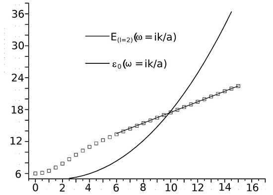
Figure 1.
Intersection of the numerically generated curves and for . Note the agreement with the results in [19], according to which for the intersection occurs at .
We close this section with two remarks. The first one concerns the behavior of the perturbation at the ring singularity. Contrary to what happens for the static NSs such as the negative mass Schwarzschild solution, or the super-extreme Reisner-Nordström solution, is not a singular point of the radial equation of the Kerr NS: the potential (57) is indeed smooth everywhere. In fact, is neither a boundary point, nor a singular point of the second order radial Equation (56), for which the domain is . Imposing any conditions at , besides requiring that the perturbations vanishes at , leads to an unnaturally over-determined problem. There is no visible effect of the ring singularity at this level. The second remark is that unstable perturbations are not restricted to the fundamental radial mode since, for large k, the potential V in (56) has a deep minimum that can be approximated by a harmonic oscillator potential of depth of order , and strength also of order , so that the level spacing near the ground state of is of order k. Thus, the negative of the lowest radial eigenvalues grow also quadratically in k for large k, and intersect the angular eigenvalue curves for sufficiently large values of k.
3.3. Instability of the Kerr Black Hole Region beyond the Cauchy Horizon
In Section 3.1, we commented that the Reissner-Nordström NS and the region beyond the Cauchy (that is, the inner) horizon of a Reissner-Nordström BH are unstable, and that the proof on instability follows similar steps as the proof of instablility of the Schwarzschild NS (see [20]) for details). In what follows we show how the proof of instability of the Kerr NS above can be adapted to prove the instability of the region of a Kerr BH. The extreme and sub-extreme cases require separate treatments.
3.3.1. Extreme Case (a = M) Inner Region:
The solution of the equation in the interior region is
its inverse is
Using the integration factor as before, we are led back to (56) and (57), with r given in (65). Note that
then the spectrum of the self-adjoint operator is again fully discrete and has a lower bound. The eigenfunctions behave as
The argument of instability that we used in for the Kerr NS goes through in this case without modifications, since the test function in (60) is supported in the region, and thus can be used again in this case to obtain the bound (62). The radial decay (67) guarantees that corrections to relevant quantities vanish in these limits. The considerations about the perturbation behavior near the ring singularity for the Kerr NS case apply verbatim to this case, and also to the sub-extreme case below.
3.3.2. Sub-Extreme Case () Inner Region:
The sub-extreme case introduces some subtleties: requiring for gives
and the radial equation reduces to (56), (57) with r the inverse of (68).
Since
Equation (56) is, in this case, a Schrödinger equation on a half axis, with potential diverging as
for . For ,
with . The eigenfunctions of behave near as
(the E eigenvalue appears in sub-leading terms). If , for generic E these are not square integrable near zero unless we choose . A case like this referred to as “limit point at ” in the classification introduced in chapter X in [25] (recall that in the case of the Schwarzschild NS we had limit circle case). In this case we need to choose to define a space of functions where is self-adjoint. This selects a discrete set of possible E values as the spectrum of . On the other hand, if , any eigenfunction (71) will be square integrable near the boundary , that is, V is limit circle at if . In this case, a choice of boundary condition, that is, a fixed value of in (71), needs to be made to define the domain of allowed perturbations. This is entirely analogous to the situation we found when studying Schwarzschild (see the discussion following Equation (40)). In this case, however, it is easy to prove that, regardless our choice for α in (71) there will be unstable modes. This is so because functions of compact support away from belong to the domain, for any , and the test function used in (60)–(61) is of compact support, so the proof of existence of an unstable mode goes through for any .
4. Nonmodal Stability of the Schwarzschild Black Hole
Prior to [36] all notions of stability of the exterior region of a Schwarzschild BH were concerned with finding bounds to the Regge-Wheeler and Zerilli fields . These fields are defined in the two dimensional orbit space and parametrize time dependent metric perturbations in the Regge-Wheeler (RW) gauge as shown in the set of equations, (12)–(27), that we will write more concisely as
where
and is a second order differential operator.
Some key results were:
- In [37], it was shown that separable solutions that do not diverge as require , ruling out exponentially growing solutions in the odd sector.
- In [38], it was shown that separable solutions that do not diverge as require , ruling out exponentially growing solutions in the even sector.
- In [39], it was shown that, for large t and fixed r, decays asan effect known as “Price tails”.
- In [40], the conserved energywas used to rule out uniform exponential growth in time.
- Furthermore, in [40], a pointwise boundwas proved, where the constants are given in terms of the initial data
To understand the limitations of these results it is important to keep in mind that the are an infinite set of fields defined on the orbit space, whose first and second order derivatives enter the terms in the series (72) through (73), together with the sheperical harmonics and their derivatives. Two extra derivatives are then required to calculate the perturbed Riemann tensor from the metric perturbation, as a first step to measure the effects of the perturbation on the curvature. Thus, the relation of the to geometrically meaningful quantities is remote, and the usefulness of the bounds (76) to measure the strength of the perturbation is not obvious at all.
Even if we knew the impact of these bounds on the components of , we would face the unavoidable problem of the lack of a natural measure of the “size” of tensor fields on a Lorentzian manifold. On a Riemannian manifold, where the metric is positive definite, the pointwise size of a tensor , could be measured by , which is positive if is nonzero, and an norm of the field given by . None of these notions is available for a Lorentzian .
Besides the problem, inherent to Lorentzian geometry, of measuring the “size” of tensors, there is the often overlooked fact that controlling the size of time dependent series terms of a quantity does not entirely control the quantity itself. This is what led to the notion of nonmodal stability in fluid dynamics, where the limitations of the mode analysis were realized in experiments involving shear flows bounded by walls [41]. In this case, the linearized Navier–Stokes operator is non normal, so their eigenfunctions are non orthogonal. As a consequence, even if the individual modes decay as —a condition that assures large t stability—there may be important transient growths [41]. Take, for example, the following toy model (from Section 2.3 in [41]) of a system with two degrees of freedoms: obeying the equation , with a matrix with (non orthogonal!) eigenvectors , say,
Consider the case . Note that, although , that is, normal modes decay exponentially, if , then reaches a maximum norm at a finite time before decaying to zero. The operators involved in the LEE are normal, so the above situation of non orthogonal eigenfunctions does not arise. However, it is easy to construct examples of, e.g., time dependent scalars on the sphere, say
where the oscillate (as the pure modes (28) were shown to do) and yet the function develops arbitrarily high localized transient growths, or even grows without bound as in continuously narrowing areas. This is so because (recall that our are an orthonormal basis of real spherical harmonics on the unit sphere )
and the integral above can be kept bounded in t while at grows high in narrowing areas. In fact, this was precisely the motivation in [40]: to “undo” the separation of variables in
and show that the sum (81) of oscillating modes does not allow unbounded transient growths in , and that we can place pointwise bounds based on the initial data of the form (76) and (77). This could be done exploiting the form of the partial differential Equation (24) obeyed by the fields . Although finding an exponentially growing mode is a definite signal of instability, as we can see, there are different possible degrees of stability when all modes are oscillating (real ’s). The symmetries of the background geometry is what allowed us to decompose metric perturbations as in (73) and (28). The results in [40] can be regarded as a way to “undo” the variable separation (28): they prove (76) and (77) for arbitrary (that is, non necessarily separable) solutions of the 1 + 1 wave Equations (24). A natural question after the work [40] is: Can we also “undo” the separation of variables? Can we find bounds for arbitrary solutions of the LEE (7)? The question is very tricky since it omits a difficult issue: which spacetime scalar field should we try to place bounds on?
The strategy in [36] was to measure the pointwise intensity of a perturbation by its effect on curvature related scalar fields (CSs, for short, not to be confused with the Newman-Penrose spin weighted scalars (33) and (34), which depend point by point on a selected null tetrad). These scalars are full contractions of the Weyl tensor (which equals the Riemann tensor in vacuum), its covariant derivatives, the metric and its inverse, and the volume form . Some examples are
Working with scalar fields avoids the issue discussed above of “measuring the size of tensors” when the background metric is Lorentzian. There is, however, the misconception that the first order variation of any CS is gauge invariant (that is, coordinate independent). This is not the case: under the transformation (9), the first order perturbation of a CS field Z changes as , so is gauge invariant if and only if the background CS vanishes: . As an example, in the Schwarzschid de Sitter (SdS) background, the CSs (82) take the values
so in the linearized theory only is a gauge invariant quantity. However, combinations of first order variations of CSs whose background values are nonzero can be gauge invariant. As an example, the field
is gauge invariant since, under a gauge transformation along ,
In [36], the fields and were proposed to measure the strength of perturbations. It was shown that:
- depends only on the odd piece of the perturbation, whereas depends only on
- There is a one to one relation between the gauge class of a metric perturbation (that is, the set of perturbations obtained from by a transformation (9)) and the . More precisely, the mapsare bijections. In particular, the gauge perturbation in, say, the RW gauge, can be recovered from the fields.
For the odd sector of the LEE, a four dimensional approach relating the metric perturbation with a scalar potential defined on the spacetime , instead of the orbit manifold, was found in [36]. It was noticed that the sum over of (73) simplifies to
where is the dual of the Weyl tensor, and is a field assembled using spherical harmonics and the :
The odd sector LEE equations for , combined with the spherical harmonic Equation (17) for the (see (24) and (27)), turn out to be equivalent to what we call the four dimensional Regge-Wheeler equation (4DRWE), which reads
Note, however, that is no more than the collection of fields : its connection to geometrically relevant fields such as CSs is, a priori, loose. Note also that any field of the form
satisfies, for arbitrary constants , the 4DRWE (89). This is a consequence of the form of the potential (see (27)), which contains an “angular momentum” term (contrast with )
Much more important is the fact (proved in [36] for , generalized to nonzero in [9]) that the LEE implies that the field can be written, after reiterated use of the LEE and equations derived from these, as
The first term contains the contribution which, as we commented above, is time independent and irrelevant to the stability problem (there is no odd contribution). This time independent contribution amounts to a shift of the Schwarzschild BH to a “slowly rotating Kerr black hole”. Technically, by “slowly rotating Kerr black hole” we mean the metric we get if we Taylor expand Kerr’s metric (1) and (2) in the rotation parameter a and keep only first order terms: for such a perturbation, looks exactly like the (rotation around the axis) term in the first sum in (91). The second term of , being of the form (90), satisfies the 4DRWE (89). What is not obvious, but can be checked by direct calculation, is that the piece of (and thus ) also satisfies (89). in (91) contains all the information we need to reconstruct the metric perturbation: the can be obtained as the harmonic coefficients of , and the (which are all we need to reconstruct the piece of the metric perturbation, see [9]) can be obtained from the coefficients. This proves that the gauge invariant, curvature scalar contains all the information encoded in an odd metric perturbation, while being a meaningful scalar to measure the strength of the perturbation. If we managed to place a pointwise bound on this quantity we would have a proof of nonmodal linear stability of the Schwarzschild BH under odd perturbations. A pointwise bound can be placed on using the fact that satisfies (89), by adapting a technique from [42] (see [9,36] for details). The result is the following: for all in the BH (or r between the event and cosmological horizons if ), and all t, there is a constant that depends on the initial datum such that
This equation settles the issue of nonmodal stability under odd perturbations.
To treat even perturbations, we must face the problem that, as becomes obvious when inspecting the even potential in (27), particularly the factors involving ℓ in the denominator, the even Equation (24) cannot be used together with (17) to construct a scalar field that satisfies a covariant equation such as the (89). A remarkable result by Chandrasekhar [27,28] comes to our help: there exists operators of the form
where
such that, if is a solution of the odd Equation (24), then is a solution of the even equation, and similarly replacing . In [9], Lemma 7, it was furthermore proved that, although the operators (93) clearly have a non trivial kernel when acting on arbitrary functions, they are 1-1 when restricted to solutions of the 1 + 1 wave Equations (24). As a consequence, every solution of the even 1 + 1 wave equation in the domain of a Schwarzschild BH (r between the event and cosmological horizons if ), can be written as .
Using the even LEE and equations derived from those, can be reduced to [36]
where
The—time-independent—first term in (95) comes from the even perturbation, which amounts to a mass shift of the background metric [9] (there is no even contribution, see [9]). Further use of the Chandrasekhar operators described above allows to rewrite entirely in terms of functions obeying (89). The details, which are quite involved, as well as the details of how to use this fact to set a bound on , can be found in [9]. We only quote the result obtained in [9,36]: for all in the BH (r between the event and cosmological horizons if ) and all t, there is a constant that depends on the initial datum such that
Together with (92), this equation proves the nonmodal linear stability of Schwarzschid BHs.
We close this sections with two observations made in [9]. Combining (91) and (95) with the Price tail decay at fixed r, Equation (74), we find that, at large t and fixed ,
which corresponds to a stationary BH in the Kerr (or Kerr de Sitter) family with a mass and angular momentum components . For example, if only , the perturbation (98) corresponds (in some gauge) to the metric perturbation obtained by applying the operator to the metric (1) and (2). Equation (98) indicates that, after a long time, the perturbation settles into a “slowly rotating” Kerr (or Kerr dS) BH. For , this fact was rigorously proved in [43], where it was shown, working in an specific gauge, that the metric perturbation decays at large t into that of a slowly rotating BH.
The second observation is that there is a much simpler CS connected to even perturbations, but this CS is not gauge invariant. This is , defined in (82) which, in the Regge-Wheeler gauge, has a first order variation [9]
Thus, , being of the form (90), also satisfies the 4DRW equation. We might think of using to measure the strength of even perturbations, but this field, as we said, is gauge dependent, due to the fact that for the background Schwarzschild or S(A)dS black hole and, as a consequence, under the gauge transformation (9),
A gauge invariant field was found in [9] for the even perturbations which satisfies the 4DRWE (89) (see the discussion in Section 5.2 of this reference). This has the drawback of not having a direct geometric interpretation in terms of CSs. In any case, we learn from the existence of , or just from Equation (99), that the degrees of freedom of the linearized even perturbations can be encoded in a scalar field satisfying the 4DRWE (89), as is the case for the odd perturbations. This field is independent from the odd field (88), that also satisfies this equation. In other words: the most general linear perturbation can be encoded in two independent scalar fields which satisfy (89). Thus, proving the stability and the large t decay of perturbations of a Schwarzschild or Schwarzschild-de Sitter BH into slowly rotating Kerr (de Sitter) BH amounts to proving the decay of the components of generic solutions of (89). This is at the heart of the proof in [43] of the decay of perturbations for , where the two scalars satisfying (89) were integrated into an symmetric tensor, as explained in Remark 7.1 in [43].
5. Conclusions and Current Developments
The proof of the instabilities of the naked singularities and the regions beyond the black hole Cauchy horizon within the Kerr–Newman family of metrics, conciliates General Relativity with basic Physics principles, such as the uniqueness of evolution from initial data, and the requirement that causal pathologies such as closed timelike and null curves do not occur. A modal analysis of the LEE is enough to rule out these solutions, given that exponentially growing modes are found. It is an interesting fact that, in the non rotating case, the geometrical effects of the unstable modes show up in differential curvature scalar invariants and in the splitting of one of the background degenerate Petrov null directions (see Equations (47) and (49)). They do not leave traces on algebraic curvature scalars, in contrast to what happens for generic black hole perturbations, (see, for example, Equations (91) and (95)). It is also interesting that the unstable modes in all the analyzed static cases (negative mass Schwarzschild NS, super extreme Reissner-Nordström NS, inner region of the Reissner-Nordström BH) are even under P, as defined in (14), and that there is exactly one unstable mode in each harmonic sector.
An analysis of these cases suggests that the singularity plays no role in the instability. As an example, for the Schwarzschild naked singularity, a negative sector of the potential in the 1 + 1 wave Equations (24)–(27) is responsible for the existence of the unstable modes. If the singularity were replaced by a small spherically symmetric negative mass distribution, away from this potential would not change substantially, and an unstable mode could be found anyway. This is also the case of the super-extreme Reisner-Nordström NS, treated in [19,20], for which the singularity could be replaced by a spherically symmetric charge distribution with leading to a non singular metric which would, anyway, be unstable. Similarly, for the Kerr NS, the ring singularity plays no role in its instability. This leaves the impression that General Relativity simply “dislikes” unusual matter or over-rotating and over-charged compact objects.
The analysis of the stability of black hole outer regions, having passed decades ago the test of modal linear stability, has had, after a long period of little activity, a remarkable progress in the last few years. An incomplete list of recent advances related to the stability of the Schwarschild and Kerr black holes follow: (i) for Schwarzschild black holes the nonmodal linear stability was established in [9,36]; (ii) in the case, the decay in time of generic linear perturbations of the Schwarzschild black hole, leaving a “slowly” rotating Kerr black hole was proved in [43]; (iii) the conditional stability of the Schwarzschild black hole, and the breaking of the even/odd symmetry mediated by the Chandrasekhar operators (93) and (94) was studied in [29]; (iv) the non-linear stability of the Schwarzschild de Sitter black hole was proved in [7]; (v) a preprint is now available with a proof of the non-linear stability of the Schwarzschild black hole [8]; (vi) pointwise decay estimates for solutions of the linearized Einstein’s equations on the outer region of a Kerr black hole were obtained in [13]; (vii) the role of hidden symmetries (see the review [44]) in type D spacetimes, and the reconstruction of (gravitational, Maxwell and spinor) perturbation fields from “Debye potentials” (first introduced in [45,46]), was studied in depth and made clear in the series of papers [47,48,49,50].
The ultimate challenge in Black Hole perturbation theory remains open: proving the non-linear stability of the outer region of a Kerr black hole.
Funding
This research was funded by CONICET (Argentina) grant PIP 11220080102479 and Universidad Nacional de Córdoba (Argentina), grant 30720110 101569CB.
Acknowledgments
This review is an outgrowth of the lecture notes for a course on linear stability of black holes and naked singularities delivered at the V José Plínio Baptista School of Cosmology, held at Guarapari (Espírito Santo) Brazil, from 30 September to 5 October 2021. I thank the organizers for giving me the opportunity of lecturing at the School.
Conflicts of Interest
The author declares no conflict of interest.
Abbreviations
References
- O’Neill, B. The Geometry of Kerr Black Holes; A K Peters: Natick, MA, USA; CRC Press: Boca Raton, FL, USA, 1992. [Google Scholar]
- Robinson, D.C. Uniqueness of the Kerr black hole. Phys. Rev. Lett. 1975, 34, 905. [Google Scholar] [CrossRef]
- Heusler, M. Black Hole Uniqueness Theorems; Cambridge Lecture Notes in Physics; Cambridge University Press: Cambridge, UK, 1996. [Google Scholar] [CrossRef]
- Friedrich, H. Existence and structure of past asymptotically simple solutions of Einstein’s field equations with positive cosmological constant. J. Geom. Phys. 1986, 3, 101–117. [Google Scholar] [CrossRef]
- Friedrich, H. On the existence of n-geodesically complete solutions of Einstein’s field equations with smooth asymptotic structure. Commun. Math. Phys. 1986, 107, 587–609. [Google Scholar] [CrossRef]
- Christodoulou, D.; Klainerman, S. The Global Nonlinear Stability of the Minkowski Space; Princeton Math. Ser. 41; Princeton University: Princeton, NJ, USA, 1993. [Google Scholar]
- Hintz, P.; Vasy, A. The global non-linear stability of the Kerr-de Sitter family of black holes. Acta Math. 2008, 220, 1–206. [Google Scholar] [CrossRef]
- Dafermos, M.; Holzegel, G.; Rodnianski, I.; Taylor, M. The non-linear stability of the Schwarzschild family of black holes. arXiv 2021, arXiv:2104.08222. [Google Scholar]
- Dotti, G. Black hole nonmodal linear stability: The Schwarzschild (A)dS cases. Class. Quantum Gravity 2016, 33, 205005. [Google Scholar] [CrossRef]
- Teukolsky, S.A. Rotating black holes—Separable wave equations for gravitational and electromagnetic perturbations. Phys. Rev. Lett. 1972, 29, 1114. [Google Scholar] [CrossRef]
- Teukolsky, S.A. Perturbations of a rotating black hole. 1. Fundamental equations for gravitational electromagnetic and neutrino field perturbations. Astrophys. J. 1973, 185, 635–647. [Google Scholar] [CrossRef]
- Whiting, B.F. Mode stability of the Kerr Black Hole. J. Math. Phys. 1989, 30, 1301. [Google Scholar] [CrossRef]
- Andersson, L.; Bäckdahl, T.; Blue, P.; Ma, S. Stability for Linearized Gravity on the Kerr Spacetime. arXiv 2019, arXiv:1903.03859. Available online: https://hal.archives-ouvertes.fr/hal-02080685 (accessed on 10 December 2021).
- Dotti, G.; Gleiser, R.J. The Initial value problem for linearized gravitational perturbations of the Schwarzchild naked singularity. Class. Quantum Gravity 2009, 26, 215002. [Google Scholar] [CrossRef]
- Gleiser, R.J.; Dotti, G. Instability of the negative mass Schwarzschild naked singularity. Class. Quantum Gravity 2006, 23, 5063–5078. [Google Scholar] [CrossRef]
- Gibbons, G.W.; Hartnoll, S.A.; Ishibashi, A. On the stability of naked singularities. Prog. Theor. Phys. 2005, 113, 963. [Google Scholar] [CrossRef]
- Dotti, G.; Gleiser, R.J.; Ranea-Sandoval, I.F.; Vucetich, H. Gravitational instabilities in Kerr space times. Class. Quantum Gravity 2008, 25, 245012. [Google Scholar] [CrossRef]
- Dotti, G.; Gleiser, R.J.; Ranea-Sandoval, I.F. Instabilities in Kerr Spacetimes. Class. Quantum Gravity 2012, 29, 095017. [Google Scholar] [CrossRef]
- Dotti, G.; Gleiser, R.J.; Pullin, J. Instability of charged and rotating naked singularities. Phys. Lett. 2007, B644, 289–293. [Google Scholar] [CrossRef]
- Dotti, G.; Gleiser, R.J. Gravitational instability of the inner static region of a Reissner-Nordstrom black hole. Class. Quantum Gravity 2010, 27, 185007. [Google Scholar] [CrossRef]
- Wald, R.M. Dynamics in non-globally hyperbolic spacetimes. J. Math. Phys. 1980, 21, 2802–2805. [Google Scholar] [CrossRef]
- Ishibashi, A.; Wald, R.M. Dynamics in nonglobally hyperbolic static space-times. 2. General analysis of prescriptions for dynamics. Class. Quantum Gravity 2003, 20, 3815. [Google Scholar] [CrossRef]
- Ishibashi, A.; Wald, R.M. Dynamics in nonglobally hyperbolic static space-times. 3. Anti-de Sitter space-time. Class. Quantum Gravity 2004, 21, 2981. [Google Scholar] [CrossRef]
- Araneda, B.; Dotti, G. Instability of asymptotically anti de Sitter black holes under Robin conditions at the timelike boundary. Phys. Rev. D 2017, 96, 104020. [Google Scholar] [CrossRef]
- Reed, M.; Simon, B. Fourier Analysis, Self-Adjointness; Methods of Modern Mathematical Physics; Academic Press: Cambridge, MA, USA, 1975; Volume 2. [Google Scholar]
- Cardoso, V.; Cavaglia, M. Stability of naked singularities and algebraically special modes. Phys. Rev. D 2006, 74, 024027. [Google Scholar] [CrossRef]
- Chandrasekhar, S. On algebraically special perturbations of black holes. Proc. R. Soc. Lond. A 1984, 392, 1. [Google Scholar]
- Chandrasekhar, S. The Mathematical Theory of Black Holes, 2nd ed.; Oxford University Press: Oxford, UK, 1992. [Google Scholar]
- Araneda, B.; Dotti, G. Petrov type of linearly perturbed type D spacetimes. Class. Quantum Gravity 2015, 32, 195013. [Google Scholar] [CrossRef]
- Cherubini, C.; Bini, D.; Bruni, M.; Perjes, Z. Petrov classification of perturbed space-times: The Kasner example. Class. Quantum Gravity 2004, 21, 4833. [Google Scholar] [CrossRef][Green Version]
- Seidel, E. A comment on the eigenvalues of spin-weighted spheroidal functions. Class. Quantum Grav. 1989, 6, 1057. [Google Scholar] [CrossRef]
- Berti, E.; Cardoso, V.; Casals, M. Eigenvalues and eigenfunctions of spin-weighted spheroidal harmonics in four and higher dimensions. Phys. Rev. D 2006, 73, 024013, Erratum in Phys. Rev. D 2006, 73, 109902. [Google Scholar] [CrossRef]
- Berti, E.; Cardoso, V.; Yoshida, S. Highly Damped Quasinormal Modes of Kerr Black Holes: A Complete Numerical Investigation. Phys. Rev. D 2004, 69, 124018. [Google Scholar] [CrossRef]
- Breuer, R.A. Gravitational Perturbation Theory and Synchrotron Radiation; Lecture Notes in Physics; Springer: Berlin/Heidelberg, Germany, 1975; Volume 44. [Google Scholar]
- Breuer, R.A.; Ryan, M.P., Jr.; Waller, S. Some properties of spin-weighted spheroidal harmonics. Proc. R. Soc. Lond. A 1977, 358, 71–86. [Google Scholar]
- Dotti, G. Nonmodal linear stability of the Schwarzschild black hole. Phys. Rev. Lett. 2014, 112, 191101. [Google Scholar] [CrossRef]
- Regge, T.; Wheeler, J.A. Stability of a Schwarzschild singularity. Phys. Rev. 1957, 108, 1063. [Google Scholar] [CrossRef]
- Zerilli, F.J. Effective potential for even parity Regge-Wheeler gravitational perturbation equations. Phys. Rev. Lett. 1970, 24, 737. [Google Scholar] [CrossRef]
- Price, R.H. Nonspherical perturbations of relativistic gravitational collapse. 1. Scalar and gravitational perturbations. Phys. Rev. D 1972, 5, 2419. [Google Scholar] [CrossRef]
- Wald, R. Note on the stability of the Schwarzschild metric. J. Math. Phys. 1979, 20, 1056, Erratum in J. Math. Phys. 1980, 21, 218. [Google Scholar] [CrossRef]
- Schmid, P.J. Nonmodal stability theory. Annu. Rev. Fluid Mech. 2007, 39, 129. [Google Scholar] [CrossRef]
- Kay, B.S.; Wald, R.M. Linear Stability Of Schwarzschild Under Perturbations Which Are Nonvanishing on the Bifurcation Two Sphere. Class. Quantum Gravity 1987, 4, 893. [Google Scholar] [CrossRef]
- Dafermos, M.; Holzegel, G.; Rodnianski, I. The linear stability of the Schwarzschild solution to gravitational perturbations. Acta Math. 2019, 222, 1–214. [Google Scholar] [CrossRef]
- Frolov, V.; Krtous, P.; Kubiznak, D. Black holes, hidden symmetries, and complete integrability. Living Rev. Relat. 2017, 20, 6. [Google Scholar] [CrossRef]
- Kegeles, L.S.; Cohen, J.M. Constructive Procedure For Perturbations Of Space-times. Phys. Rev. D 1979, 19, 1641. [Google Scholar] [CrossRef]
- Wald, R.M. Construction of Solutions of Gravitational, Electromagnetic, Or Other Perturbation Equations from Solutions of Decoupled Equations. Phys. Rev. Lett. 1978, 41, 203. [Google Scholar] [CrossRef]
- Araneda, B. Symmetry operators and decoupled equations for linear fields on black hole spacetimes. Class. Quantum Gravity 2017, 34, 035002. [Google Scholar] [CrossRef]
- Araneda, B. Generalized wave operators, weighted Killing fields, and perturbations of higher dimensional spacetimes. Class. Quantum Gravity 2018, 35, 075015. [Google Scholar] [CrossRef]
- Araneda, B. Conformal invariance, complex structures and the Teukolsky connection. Class. Quantum Gravity 2018, 35, 175001. [Google Scholar] [CrossRef]
- Araneda, B. Two-dimensional twistor manifolds and Teukolsky operators. Lett. Math. Phys. 2020, 110, 2603–2638. [Google Scholar] [CrossRef]

Publisher’s Note: MDPI stays neutral with regard to jurisdictional claims in published maps and institutional affiliations. |
© 2022 by the author. Licensee MDPI, Basel, Switzerland. This article is an open access article distributed under the terms and conditions of the Creative Commons Attribution (CC BY) license (https://creativecommons.org/licenses/by/4.0/).