On the Constant-Roll Inflation with Large and Small η_H

Abstract

We study the apparent duality between large and small ${\eta }_H$ for the constant-roll inflation with the second slow-roll parameter ${\eta }_H$ being a constant. In the previous studies, only the constant-roll inflationary models with small ${\eta }_H$ are found to be consistent with the observations. The apparent duality suggests that the constant-roll inflationary models with large ${\eta }_H$ may be also consistent with the observations. We find that the duality between the constant-roll inflation with large and small ${\eta }_H$ does not exist, because both the background and scalar perturbation evolutions are very different. By fitting the constant-roll inflationary models to the observations, we get $-0.016\le {\eta }_H\le -0.0078$ at the 95% C.L if we take $N=60$ for the models with increasing ${ϵ}_H$, in which inflation ends when ${ϵ}_H=1$. For the models with decreasing ${ϵ}_H$, we obtain $3.0135\le {\eta }_H\le 3.021$ at the 68% C.L. and $3.0115\le {\eta }_H\le 3.024$ at the 95% C.L.

1. Introduction

Inflation explains the flatness and horizon problems in standard cosmology [1,2,3,4], and the quantum fluctuations of the inflaton seed the large scale structure of the Universe and leave imprints on the cosmic microwave background radiation [5,6,7,8]. To solve problems such as the flatness, horizon, and monopole problems, the number of e-folds remaining before the end of inflation must be large enough, and it is usually taken to be $N=50-60$ due to the uncertainties in reheating physics. This requires the potential of the inflaton to be nearly flat, i.e., the slow-roll inflation. The temperature and polarization measurements on the cosmic microwave background anisotropy conformed the nearly scale invariant power spectra predicted by the slow-roll inflation and gave the constraints $n_s=0.965\pm 0.004$ (68% C.L.) and $r_{0.05}<0.06$ (95% C.L.) [9,10].

Recently, the constant-roll inflation with ${\eta }_H$ being a constant [11,12] attracted some attention, because the inflationary potential and the background equation of motion can be solved analytically. The slow-roll parameter ${\eta }_H$ is a constant and it may not be small, so the model is different from the typical slow-roll inflationary models. In particular, when the inflationary potential becomes very flat, ${\eta }_H=3$, we get the ultra-slow-roll inflation [13,14]. Due to the violation of the slow-roll condition in the constant-roll inflationary models with large ${\eta }_H$, the curvature perturbation may evolve outside the horizon and the slow-roll results may not be applied [11,12,14,15,16,17,18,19]. However, for the constant-roll inflation with ${\eta }_H>1$, the slow-roll parameter ${ϵ}_H$ decreases with time and is small during inflation, so we can still use the standard method of Bessel function approximation to calculate the power spectra. Neglecting the contribution from ${ϵ}_H$, it was found there exists a duality between the ultra-slow-roll inflation and the slow-roll inflation [20,21,22], i.e., if we replace ${\eta }_H$ by ${\overline{\eta }}_H=3-{\eta }_H$, we get the same result for the scalar spectral tilt. Recall that the observational data constrained ${\eta }_H$ to be small [23,24,25]; these results are in conflict with the duality relation, so it is necessary to revisit the observational constraint to include the constraint on the ultra-slow inflation. For the ultra-slow-roll inflation, it is legitimate to neglect ${ϵ}_H$. For the typical slow-roll inflation, ${ϵ}_H$ and ${\eta }_H$ are in the same order, so ${ϵ}_H$ cannot be neglected and it is interesting to discuss the duality up to the first order of ${ϵ}_H$ in the constant-roll inflation. The difference in ${ϵ}_H$ may cause different amplitudes for the power spectra or different energy scale of inflation. Furthermore, due to the smallness of ${ϵ}_H$ in the ultra-slow-roll inflation, it can be used to generate a large curvature perturbation at small scales, which produces primordial black holes and secondary gravitational waves [26,27,28,29]. For more discussion on the constant-roll inflation, see, e.g., in [30,31,32,33,34,35,36,37,38,39,40,41,42].

In this paper, we extend the discussion of the duality between the ultra-slow-roll inflation and the slow-roll inflation with constant ${\eta }_H$ to include the effect of ${ϵ}_H$. The paper is organized as follows. In Section 2, we review the constant-roll inflation and discuss the duality between the ultra-slow-roll inflation with large constant ${\eta }_H$ and the slow-roll inflation with small constant ${\eta }_H$. In Section 3, we fit constant-roll models to the observational data. The conclusions are drawn in Section 4.

2. The Constant-Roll Inflation

We use the Hubble flow slow-roll parameters [43],

$${}^n{\beta }_H=2{\left(\frac{{\left(H_{,\varphi }\right)}^{n-1}{H}_{,\varphi }^{(n+1)}}{H^n}\right)}^{1/n},$$

(1)

where $H_{,\varphi }=dH/d\varphi$ and $H_{,\varphi }^{\left(n\right)}=d^{n}H/d{\varphi }^n$. In particular, the first three slow-roll parameters are

$${ϵ}_H=2{\left(\frac{H_{,\varphi }}{H}\right)}^2=-\frac{\dot{H}}{H^2},$$

(2)

$${\eta }_H=\frac{2H_{,\varphi }^{\left(2\right)}}{H}=-\frac{\ddot{\varphi }}{H\dot{\varphi }}=-\frac{\ddot{H}}{2H\dot{H}},$$

(3)

$${\xi }_H=\frac{4H_{,\varphi }{H}_{,\varphi }^{\left(3\right)}}{H^2}=\frac{\stackrel{⃛}{H}}{2H^2\dot{H}}-2{\eta }_H^2,$$

(4)

and the evolution of the slow-roll parameters are

$${\dot{ϵ}}_H=2H{ϵ}_H({ϵ}_H-{\eta }_H),$$

(5)

$${\dot{\eta }}_H=H({ϵ}_H{\eta }_H-{\xi }_H),$$

(6)

where $\dot{H}=dH/dt$. For the constant-roll inflation with constant ${\eta }_H$, we get ${\xi }_H={ϵ}_H{\eta }_H$. From Equation (5), we see that if ${ϵ}_H>{\eta }_H$, then ${ϵ}_H$ increases monotonically with time. Otherwise, if ${ϵ}_H<{\eta }_H$, then ${ϵ}_H$ decreases monotonically with time. As ${ϵ}_H\le 1$, ${ϵ}_H$ decreases monotonically with time for the constant-roll inflationary model with ${\eta }_H>1$, such as the ultra-slow-roll inflation with ${\eta }_H\approx 3$.

The scalar perturbation is governed by Mukhanov–Sasaki equation [44,45],

$$v_k^{″}+\left(k^2-\frac{z^{″}}{z}\right)v_k=0,$$

(7)

where

$$z=\frac{a\dot{\varphi }}{H},$$

(8)

$v_k^{\prime }=d{v}_k/d\tau$, $\tau$ is the conformal time, and the mode function $v_k$ for a Fourier mode is related with the curvature perturbation $\zeta$ by $v_k=z{\zeta }_k$. To the first order of ${ϵ}_H$, $aH\approx -(1+{ϵ}_H)/\tau$, and Equation (7) becomes

$$v_k^{″}+\left(k^2-\frac{{\nu }^2-1/4}{{\tau }^2}\right)v_k=0,$$

(9)

where

$$\nu \approx \frac{1}{2}|2{\eta }_H-3|+\frac{(2{\eta }_H^2-9{\eta }_H+6){ϵ}_H}{|2{\eta }_H-3|}.$$

(10)

As ${\eta }_H$ is a constant and the change of ${ϵ}_H$ can be neglected which is true for both slow-roll and ultra-slow-roll inflation 1, so $\nu$ can be approximated as a constant, the solution to Equation (9) for the mode function $v_k$ is the Hankel function of order $\nu$,

$$v_k=\frac{\sqrt{\pi }}{2}{e}^{i(\nu +1/2)\pi /2}\sqrt{-\tau }{H}_{\nu }^{\left(1\right)}(-k\tau ).$$

(11)

Therefore, the power spectrum of the scalar perturbation is

$$\begin{array}{cc}\hfill P_{\zeta }& =\frac{k^3}{2{\pi }^2}{\left|{\zeta }_k\right|}^2\hfill \\ \hfill & =\frac{2^{2\nu -3}}{2{ϵ}_H}{\left[\frac{\Gamma \left(\nu \right)}{\Gamma (3/2)}\right]}^2{\left(1+{ϵ}_H\right)}^{1-2\nu }{\left(\frac{H}{2\pi }\right)}^2{\left(\frac{k}{aH}\right)}^{3-2\nu }.\hfill \end{array}$$

(12)

The amplitude of the power spectrum at the horizon crossing is

$$A_s=\frac{2^{2\nu -3}}{2{ϵ}_H}{\left[\frac{\Gamma \left(\nu \right)}{\Gamma (3/2)}\right]}^2{\left(1+{ϵ}_H\right)}^{1-2\nu }{\left(\frac{H}{2\pi }\right)}^2.$$

(13)

The scalar spectral tilt is

$$\begin{array}{cc}\hfill n_s-1& =\frac{dln{P}_{\zeta }}{dlnk}\hfill \\ \hfill & \approx 3-|2{\eta }_H-3|-\frac{2(2{\eta }_H^2-9{\eta }_H+6){ϵ}_H}{|2{\eta }_H-3|}.\hfill \end{array}$$

(14)

Following the same procedure, we get the power spectrum of the tensor perturbation and the tensor to scalar ratio:

$$r\approx 2^{3-|2{\eta }_H-3|}{\left(\frac{\Gamma [3/2]}{\Gamma \left[\right|2{\eta }_H-3|/2]}\right)}^{2}16{ϵ}_H.$$

(15)

If we neglect the contribution of ${ϵ}_H$ in Equations (10), (14), and (15), we see that these expressions are unchanged if we replace ${\eta }_H$ by ${\overline{\eta }}_H=3-{\eta }_H$, i.e., there exists a duality between ${\eta }_H$ and ${\overline{\eta }}_H=3-{\eta }_H$ as observed in [20,21]. It this duality is true, then we can apply the usual slow-roll results to ultra-slow-roll inflationary models. In the previous analysis of the observational constraints on constant-roll inflation, only the model with small ${\eta }_H$ was found to be consistent with the observations [19,23,24,25]. This duality relation suggests that the ultra-slow-roll inflationary models may also be consistent with the observations. To investigate whether this is true, we discuss the issue of duality below.

2.1. The Constant-Roll Models

From Equation (3), we get

$$H\left(\varphi \right)=c_{1}exp\left(\sqrt{\frac{{\eta }_H}{2}}\varphi \right)+c_{2}exp\left(-\sqrt{\frac{{\eta }_H}{2}}\varphi \right),$$

(16)

for ${\eta }_H>0$. For ${\eta }_H<0$, the general solution is the form of trigonometric functions $sin\left(x\right)$ and $cos\left(x\right)$. Following the authors of [12], for ${\eta }_H>0$, we consider the particular solutions

$$H\left(\varphi \right)=Mcosh\left(\sqrt{\frac{{\eta }_H}{2}}\varphi \right),$$

(17)

with the potential $V=3H^2-2{\left(H_{,\varphi }\right)}^2$,

$$V\left(\varphi \right)=M^2\left[3{cosh}^2\left(\sqrt{\frac{{\eta }_H}{2}}\varphi \right)-{\eta }_H{sinh}^2\left(\sqrt{\frac{{\eta }_H}{2}}\varphi \right)\right],$$

(18)

and

$$\begin{array}{c}H\left(\varphi \right)=Msinh\left(\sqrt{\frac{{\eta }_H}{2}}\varphi \right),\end{array}$$

(19)

$$\begin{array}{c}V\left(\varphi \right)=M^2\left[3{sinh}^2\left(\sqrt{\frac{{\eta }_H}{2}}\varphi \right)-{\eta }_H{cosh}^2\left(\sqrt{\frac{{\eta }_H}{2}}\varphi \right)\right].\end{array}$$

(20)

For ${\eta }_H<0$, the particular solutions are

$$\begin{array}{c}H\left(\varphi \right)=Mcos\left(\sqrt{\frac{-{\eta }_H}{2}}\varphi \right),\end{array}$$

(21)

$$\begin{array}{c}V\left(\varphi \right)=M^2\left[3{cos}^2\left(\sqrt{\frac{-{\eta }_H}{2}}\varphi \right)+{\eta }_H{sin}^2\left(\sqrt{\frac{-{\eta }_H}{2}}\varphi \right)\right],\end{array}$$

(22)

and

$$\begin{array}{c}H\left(\varphi \right)=Msin\left(\sqrt{\frac{-{\eta }_H}{2}}\varphi \right),\end{array}$$

(23)

$$\begin{array}{c}V\left(\varphi \right)=M^2\left[3{sin}^2\left(\sqrt{\frac{-{\eta }_H}{2}}\varphi \right)+{\eta }_H{cos}^2\left(\sqrt{\frac{-{\eta }_H}{2}}\varphi \right)\right].\end{array}$$

(24)

To check if we missed any background solution, we consider the solution 2 [21]

$$\begin{array}{c}\varphi \left(t\right)=2\sqrt{\frac{2}{\left|\gamma \right|}}arctan[exp(-\gamma H_{0}t)],\end{array}$$

(25)

$$\begin{array}{cc}\hfill V\left(\varphi \right)=& H_0^2\left[3{cos}^2\left(\sqrt{\frac{\left|\gamma \right|}{2}}\varphi \right)-\gamma {sin}^2\left(\sqrt{\frac{\left|\gamma \right|}{2}}\varphi \right)\right]\hfill \\ & =\frac{H_0^2(3{sinh}^2\left(\gamma H_{0}t\right)-\beta )}{{cosh}^2\left(\gamma H_{0}t\right)}.\hfill \end{array}$$

(26)

If we take $\gamma =3+\alpha$, we get the branch 1 solution given by Equations (61) and (63) in [21]. If we take $\gamma =-\alpha$, we get the branch 2 solution given by Equations (62) and (64) in [21]. Combining Equations (25) and (26), we get

$$H^2=\frac{H_0^2}{3}\left[\left(\frac{{\gamma }^2}{\left|\gamma \right|}-\gamma \right)+\left(3+\gamma -\frac{{\gamma }^2}{\left|\gamma \right|}\right){tanh}^2\left(\gamma H_{0}t\right)\right],$$

(27)

and

$$\ddot{\varphi }+\frac{dV}{d\varphi }=2H_0^2\left(\frac{{\gamma }^2}{\sqrt{2\left|\gamma \right|}}-(3+\gamma )\sqrt{\frac{\left|\gamma \right|}{2}}\right)\frac{sinh\left(\gamma H_{0}t\right)}{{cosh}^2\left(\gamma H_{0}t\right)}.$$

(28)

However, for all possible values of $\gamma$, the background equation $\ddot{\varphi }+3H\dot{\varphi }+dV/d\varphi =0$ cannot be satisfied. Therefore, Equations (61)–(64), given in [21], are not background solutions. The possible background solutions with the trigonometric function are given by Equations (21)–(24) and they are valid for ${\eta }_H<0$ only.

For the constant-roll inflation, $H\left(\varphi \right)$ is known, so we obtain the potential $V\left(\varphi \right)=3H^2-2{\left(H_{,\varphi }\right)}^2$ and $\dot{\varphi }$ is determined from the relation $\dot{\varphi }=-2H_{,\varphi }$ 3. We don’t consider the exponential solution because the corresponding power-law inflation is excluded by the observations. The models (18) and (22) were studied in [12,21,23,24]. For the model (18), ${\dot{ϵ}}_H<0$, so we need to introduce some mechanism to end inflation. The model (20) was studied in [19]. As discussed in [19], in the model (20), ${\dot{ϵ}}_H>0$ and ${ϵ}_H>{\eta }_H$, so there is no inflation in this model if ${\eta }_H>1$, i.e., the model cannot support ultra-slow-roll inflation and it is not applicable to the discussion of the duality relation.

2.2. The Duality between the Slow-Roll and the Ultra Slow-Roll Inflation

For the slow-roll inflation with ${\eta }_H=\alpha$ and $\left|\alpha \right|\ll 1$, we get

$$A_s=\frac{1}{2{ϵ}_H}{\left(\frac{H}{2\pi }\right)}^2,$$

(29)

$$n_s-1=2\alpha -4{ϵ}_H,$$

(30)

and

$$r=16{ϵ}_H.$$

(31)

For the ultra-slow-roll inflation with ${\eta }_H=3-\alpha$ and $\left|\alpha \right|\ll 1$, we get

$$A_s=\frac{1}{2{ϵ}_H}{\left(\frac{H}{2\pi }\right)}^2,$$

(32)

$$n_s-1=2\alpha +2{ϵ}_H,$$

(33)

and

$$r=16{ϵ}_H.$$

(34)

From Equation (33), we see that to be consistent with the observations $n_s<1$, we must take $\alpha <0$ because ${ϵ}_H>0$, so the constant-roll inflation with ${\eta }_H\gtrsim 3$ may be consistent with the observations.

Equations (29) and (32) show that the amplitudes of the power spectra for both the slow-roll and ultra-slow-roll inflation have the same form. From Equations (30) and (33), we see that the power spectra for both the slow-roll and ultra-slow-roll inflation are nearly scale invariant. If we neglect ${ϵ}_H$ in Equations (30) and (33), the expressions for the slow-roll inflation with ${\eta }_H=\alpha$ and the ultra-slow-roll inflation with ${\eta }_H=3-\alpha$ are the same, so it seems that there exists a duality between ${\eta }_H$ and ${\overline{\eta }}_H=3-{\eta }_H$. In particular, the model (18) is self-dual when $0\le {\eta }_H\le 3$.

If the duality holds, then the model (18) with ${\eta }_H>3$ is dual to the model (22) with ${\eta }_H<0$. However, the two potentials (18) and (22) and the background evolutions are totally different, and ${\dot{ϵ}}_H<0$ for the model (18), whereas ${\dot{ϵ}}_H>0$ for the model (22). For the model (18) with ${\eta }_H>3$, the inflation climbs up instead of rolling down the potential and the constant-roll inflationary solution is not an transactor [12]. Furthermore, as shown in [12], in the model (18) with ${\eta }_H>3/2$, the curvature perturbation grows on both the subhorizon and superhorizon scales, but the curvature perturbation decreases on the subhorizon scales and is frozen on the superhorizon scales in both the model (18) with ${\eta }_H<1$ and the model (22) as shown in Figure 1 and Figure 2, so this duality is false because the behaviors of the background and the curvature perturbations are totally different for the constant-roll inflation with large and small ${\eta }_H$. In Figure 1, we also see that the analytical power spectrum (12) for the scalar perturbation approximates the exact result very well even when ${\eta }_H>3$ and the curvature perturbations grow on superhorizon scales. Due to the growth of the curvature perturbations on superhorizon scales for the constant-roll model (18) with ${\eta }_H>3/2$, the scalar power spectrum (12) should be evaluated at the end of inflation instead of the horizon crossing [18,46,47,48,49]. This brings a new problem on the evaluation of the power spectrum, because inflation does not end naturally and some unknown mechanisms need to be introduced to end inflation in the model (18), but this problem does not exist in the model (22). For the model (20), because no inflation happens if ${\eta }_H>1$, the duality is inapplicable to this model. For the same reason, the model (24) is not dual to the model (20).

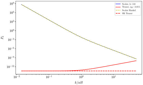
Figure 1. The scalar and tensor power spectra for the model (18) with ${\eta }_H=3.015$. The solid lines are for the numerical results. The yellow dashed line is the result obtained using the approximate formulae (11) with the Hankel function, and the red dashed line denotes the asymptotic result with the slow-roll approximation.

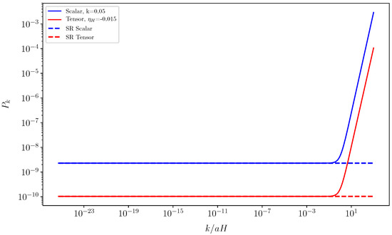
Figure 2. The scalar and tensor power spectra for the model (22) with ${\eta }_H=-0.015$. The solid lines are for the numerical results, and the dashed lines denote the asymptotic results with the slow-roll approximation.

Furthermore, ${ϵ}_H$ is usually not negligible for the slow-roll inflation, whereas it may be negligible for the ultra-slow-roll inflation, the amplitudes (29) and (32) for both the scalar and tensor spectra will be different when the effect of ${ϵ}_H$ is included, so there is no duality in the constant-roll inflation with large ${\eta }_H\approx 3$ and small ${\eta }_H\approx 0$. In particular, for the ultra-slow-roll inflation, the scalar perturbation may be very large and the tensor to scalar ratio r may be negligible.

3. The Observational Constraints

For the slow-roll inflation, in terms of the remaining number of e-folds N before the end of inflation, from Equation (5), we get

$${ϵ}_H\left(N\right)=\frac{{\eta }_H{e}^{2{\eta }_{H}N}}{-1+{\eta }_H+e^{2{\eta }_{H}N}},$$

(35)

where we impose the condition of the end of inflation ${ϵ}_H(N=0)=1$. This formulae only applies to the model with ${\dot{ϵ}}_H>0$, like the model (20).

For the ultra-slow-roll inflation, ${ϵ}_H$ decreases monotonically with time and inflation ends, and we need some mechanisms to end inflation. Instead of using N, we introduce the number of e-folds $\overline{N}$ after the start of inflation [24]. From Equation (5), we get

$${ϵ}_H\left(\overline{N}\right)=\frac{{\eta }_H}{1+e^{2{\eta }_H(\overline{N}+C)}},$$

(36)

where C is an integration constant. Take $N^{\prime }=\overline{N}+C$, we get

$${ϵ}_H\left(\overline{N}\right)=\frac{{\eta }_H}{1+e^{2{\eta }_H{N}^{\prime }}}.$$

(37)

Substituting Equation (35) into Equations (14) and (15), we can calculate $n_s$ and r for the constant-roll inflation with increasing ${ϵ}_H$. Substituting Equation (37) into Equations (14) and (15), we can calculate $n_s$ and r for the constant-roll inflation with decreasing ${ϵ}_H$. The results along with the Planck 2018 and BICEP2 constraints [9,10] are shown in Figure 3. In Figure 3, the black lines represent the calculated results with Equation (35), and the blue lines denote the calculated results with Equation (37). The model with increasing ${ϵ}_H$ is excluded by the observations if we take $N=50$ (the solid black line) and is marginally consistent with the observations at the 95% level if we take $N=60$ (the dashed black line). The constraint is $-0.016\le {\eta }_H\le -0.0078$ at the 95% C.L for $N=60$. The model with decreasing ${ϵ}_H$ is consistent with the observations, we find that $N^{\prime }\le 1.055$ at the 68% C.L. and $N^{\prime }\le 1.121$ at the 95% C.L. The constraints on the parameters ${\eta }_H$ and $N^{\prime }$ for the model (37) are shown in Figure 4. We get $3.0135\le {\eta }_H\le 3.021$ at the 68% C.L., and $3.0115\le {\eta }_H\le 3.024$ at the 95% C.L. These results show that there is no duality between ${\eta }_H$ and ${\overline{\eta }}_H=3-{\eta }_H$.

Figure 3. The marginalized 68% and 95% confidence level contours for $n_s$ and r from Planck 2018 and BICEP2 results [9,10], and the observational constraints on the constant-roll inflationary models. The black lines represent the model Equation (35) and the blue lines denote the model Equation (37).

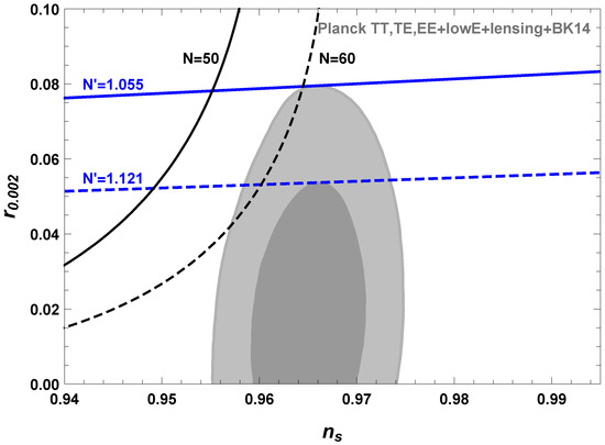
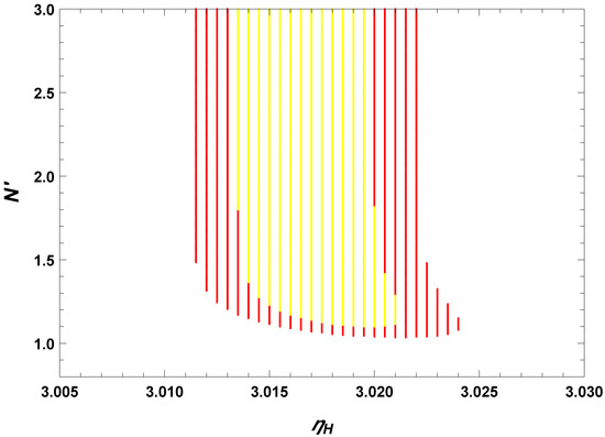
Figure 4. The observational constraints on ${\eta }_H$ and $N^{\prime }$. The yellow and red regions correspond to the 68% and 95% C.L.s, respectively.

4. Conclusions

For constant-roll inflation with large ${\eta }_H$, the slow-roll condition ${\eta }_H\ll 1$ is violated, but Hankel function can be used to approximate the solution to Mukhanov–Sasaki equation and analytical formulae for the power spectrum can be obtained. We show that the analytical formulae for constant-roll inflation approximates the scalar power spectrum very well even when ${\eta }_H$ is large and curvature perturbations grow on superhorizon scales. To the first order of ${ϵ}_H$, the formulae for the observables $n_s$ and r are also derived and they are valid for any constant ${\eta }_H$. Although there exists duality in the observables $n_s$ and r, the apparent duality between the constant-roll inflation with large and small ${\eta }_H$ does not exist due to different behaviors of background and scalar perturbations.

By fitting the constant-roll models to the observations, we find that the model with increasing ${ϵ}_H$ is excluded by the observations if we take $N=50$. If we take $N=60$, the constraint is $-0.016\le {\eta }_H\le -0.0078$ at the 95% C.L. For the models with decreasing ${ϵ}_H$, we obtain that $3.0135\le {\eta }_H\le 3.021$ at the 68% C.L. and $3.0115\le {\eta }_H\le 3.024$ at the 95% C.L. The inflation solution for ${\eta }_H>3$ is not an attractor, so we need to fine tune the initial conditions to get the constant-roll inflation with ${\eta }_H>3$. These results confirm that the duality between ${\eta }_H$ and ${\overline{\eta }}_H=3-{\eta }_H$ does not exist.

References

- Starobinsky, A.A. A New Type of Isotropic Cosmological Models Without Singularity. Phys. Lett. B 1980, 91, 99–102. [Google Scholar] [CrossRef]
- Guth, A.H. The Inflationary Universe: A Possible Solution to the Horizon and Flatness Problems. Phys. Rev. D 1981, 23, 347–356. [Google Scholar] [CrossRef]
- Linde, A.D. A New Inflationary Universe Scenario: A Possible Solution of the Horizon, Flatness, Homogeneity, Isotropy and Primordial Monopole Problems. Phys. Lett. B 1982, 108, 389–393. [Google Scholar] [CrossRef]
- Albrecht, A.; Steinhardt, P.J. Cosmology for Grand Unified Theories with Radiatively Induced Symmetry Breaking. Phys. Rev. Lett. 1982, 48, 1220–1223. [Google Scholar] [CrossRef]
- Mukhanov, V.F.; Chibisov, G.V. Quantum Fluctuation and Nonsingular Universe. JETP Lett. 1981, 33, 532–535. (In Russian) [Google Scholar]
- Hawking, S.W. The Development of Irregularities in a Single Bubble Inflationary Universe. Phys. Lett. B 1982, 115, 295–297. [Google Scholar] [CrossRef]
- Starobinsky, A.A. Dynamics of Phase Transition in the New Inflationary Universe Scenario and Generation of Perturbations. Phys. Lett. B 1982, 117, 175–178. [Google Scholar] [CrossRef]
- Guth, A.H.; Pi, S.Y. Fluctuations in the New Inflationary Universe. Phys. Rev. Lett. 1982, 49, 1110–1113. [Google Scholar] [CrossRef]
- Akrami, Y.; Arroja, F.; Ashdown, M.; Aumont, J.; Baccigalupi, C.; Ballardini, M.; Banday, A.J.; Barreiro, R.B.; Bartolo, N.; Basak, S.; et al. Planck 2018 results. X. Constraints on inflation. arXiv 2018, arXiv:1807.06211. [Google Scholar]
- Array, K. BICEP2/Keck Array x: Constraints on Primordial Gravitational Waves using Planck, WMAP, and New BICEP2/Keck Observations through the 2015 Season. Phys. Rev. Lett. 2018, 121, 221301. [Google Scholar]
- Martin, J.; Motohashi, H.; Suyama, T. Ultra Slow-Roll Inflation and the non-Gaussianity Consistency Relation. Phys. Rev. D 2013, 87, 023514. [Google Scholar] [CrossRef]
- Motohashi, H.; Starobinsky, A.A.; Yokoyama, J. Inflation with a constant rate of roll. J. Cosmol. Astropart. Phys. 2015, 1509, 018. [Google Scholar] [CrossRef]
- Tsamis, N.C.; Woodard, R.P. Improved estimates of cosmological perturbations. Phys. Rev. D 2004, 69, 084005. [Google Scholar] [CrossRef]
- Kinney, W.H. Horizon crossing and inflation with large eta. Phys. Rev. D 2005, 72, 023515. [Google Scholar] [CrossRef]
- Leach, S.M.; Liddle, A.R. Inflationary perturbations near horizon crossing. Phys. Rev. D 2001, 63, 043508. [Google Scholar] [CrossRef]
- Leach, S.M.; Sasaki, M.; Wands, D.; Liddle, A.R. Enhancement of superhorizon scale inflationary curvature perturbations. Phys. Rev. D 2001, 64, 023512. [Google Scholar] [CrossRef]
- Jain, R.K.; Chingangbam, P.; Sriramkumar, L. On the evolution of tachyonic perturbations at super-Hubble scales. J. Cosmol. Astropart. Phys. 2007, 0710, 003. [Google Scholar] [CrossRef][Green Version]
- Namjoo, M.H.; Firouzjahi, H.; Sasaki, M. Violation of non-Gaussianity consistency relation in a single field inflationary model. Europhys. Lett. 2013, 101, 39001. [Google Scholar] [CrossRef]
- Yi, Z.; Gong, Y. On the constant-roll inflation. J. Cosmol. Astropart. Phys. 2018, 1803, 052. [Google Scholar] [CrossRef]
- Tzirakis, K.; Kinney, W.H. Inflation over the hill. Phys. Rev. D 2007, 75, 123510. [Google Scholar] [CrossRef]
- Morse, M.J.P.; Kinney, W.H. Large-η constant-roll inflation is never an attractor. Phys. Rev. D 2018, 97, 123519. [Google Scholar] [CrossRef]
- Lin, W.C.; Morse, M.J.P.; Kinney, W.H. Dynamical Analysis of Attractor Behavior in Constant Roll Inflation. J. Cosmol. Astropart. Phys. 2019, 1909, 063. [Google Scholar] [CrossRef]
- Motohashi, H.; Starobinsky, A.A. Constant-roll inflation: confrontation with recent observational data. Europhys. Lett. 2017, 117, 39001. [Google Scholar] [CrossRef]
- Galvez Ghersi, J.T.; Zucca, A.; Frolov, A.V. Observational Constraints on Constant Roll Inflation. J. Cosmol. Astropart. Phys. 2019, 1905, 030. [Google Scholar] [CrossRef]
- Gao, Q. The observational constraint on constant-roll inflation. Sci. China Phys. Mech. Astron. 2018, 61, 070411. [Google Scholar] [CrossRef]
- Germani, C.; Prokopec, T. On primordial black holes from an inflection point. Phys. Dark Univ. 2017, 18, 6–10. [Google Scholar] [CrossRef]
- Motohashi, H.; Hu, W. Primordial Black Holes and Slow-Roll Violation. Phys. Rev. D 2017, 96, 063503. [Google Scholar] [CrossRef]
- Di, H.; Gong, Y. Primordial black holes and second order gravitational waves from ultra-slow-roll inflation. J. Cosmol. Astropart. Phys. 2018, 1807, 007. [Google Scholar] [CrossRef]
- Lu, Y.; Gong, Y.; Yi, Z.; Zhang, F. Constraints on primordial curvature perturbations from primordial black hole dark matter and secondary gravitational waves. arXiv 2019, arXiv:1907.11896. [Google Scholar]
- Motohashi, H.; Starobinsky, A.A. f(R) constant-roll inflation. Eur. Phys. J. C 2017, 77, 538. [Google Scholar] [CrossRef]
- Oikonomou, V.K. Reheating in Constant-roll F(R) Gravity. Mod. Phys. Lett. A 2017, 32, 1750172. [Google Scholar] [CrossRef]
- Odintsov, S.D.; Oikonomou, V.K. Inflation with a Smooth Constant-Roll to Constant-Roll Era Transition. Phys. Rev. D 2017, 96, 024029. [Google Scholar] [CrossRef]
- Nojiri, S.; Odintsov, S.D.; Oikonomou, V.K. Constant-roll Inflation in F(R) Gravity. Class. Quant. Grav. 2017, 34, 245012. [Google Scholar] [CrossRef]
- Dimopoulos, K. Ultra slow-roll inflation demystified. Phys. Lett. B 2017, 775, 262–265. [Google Scholar] [CrossRef]
- Ito, A.; Soda, J. Anisotropic Constant-roll Inflation. Eur. Phys. J. C 2018, 78, 55. [Google Scholar] [CrossRef]
- Karam, A.; Marzola, L.; Pappas, T.; Racioppi, A.; Tamvakis, K. Constant-Roll (Quasi-)Linear Inflation. J. Cosmol. Astropart. Phys. 2018, 1805, 011. [Google Scholar] [CrossRef]
- Fei, Q.; Gong, Y.; Lin, J.; Yi, Z. The reconstruction of tachyon inflationary potentials. J. Cosmol. Astropart. Phys. 2017, 1708, 018. [Google Scholar] [CrossRef]
- Cicciarella, F.; Mabillard, J.; Pieroni, M. New perspectives on constant-roll inflation. J. Cosmol. Astropart. Phys. 2018, 1801, 024. [Google Scholar] [CrossRef]
- Anguelova, L.; Suranyi, P.; Wijewardhana, L.C.R. Systematics of Constant Roll Inflation. J. Cosmol. Astropart. Phys. 2018, 1802, 004. [Google Scholar] [CrossRef]
- Gao, Q.; Gong, Y.; Fei, Q. Constant-roll tachyon inflation and observational constraints. J. Cosmol. Astropart. Phys. 2018, 1805, 005. [Google Scholar] [CrossRef]
- Mohammadi, A.; Saaidi, K. Constant-roll approach to non-canonical inflation. arXiv 2018, arXiv:1803.01715. [Google Scholar]
- Pattison, C.; Vennin, V.; Assadullahi, H.; Wands, D. The attractive behavior of ultra-slow-roll inflation. J. Cosmol. Astropart. Phys. 2018, 1808, 048. [Google Scholar] [CrossRef]
- Liddle, A.R.; Parsons, P.; Barrow, J.D. Formalizing the slow roll approximation in inflation. Phys. Rev. D 1994, 50, 7222–7232. [Google Scholar] [CrossRef]
- Mukhanov, V.F. Gravitational Instability of the Universe Filled with a Scalar Field. JETP Lett. 1985, 41, 493–496. [Google Scholar]
- Sasaki, M. Large Scale Quantum Fluctuations in the Inflationary Universe. Prog. Theor. Phys. 1986, 76, 1036. [Google Scholar] [CrossRef]
- Cheng, S.L.; Lee, W.; Ng, K.W. Numerical study of pseudoscalar inflation with an axion-gauge field coupling. Phys. Rev. D 2016, 93, 063510. [Google Scholar] [CrossRef]
- Cheng, S.L.; Lee, W.; Ng, K.W. Superhorizon curvature perturbation in ultraslow-roll inflation. Phys. Rev. D 2019, 99, 063524. [Google Scholar] [CrossRef]
- Byrnes, C.T.; Cole, P.S.; Patil, S.P. Steepest growth of the power spectrum and primordial black holes. J. Cosmol. Astropart. Phys. 2019, 1906, 028. [Google Scholar] [CrossRef]
- Passaglia, S.; Hu, W.; Motohashi, H. Primordial black holes and local non-Gaussianity in canonical inflation. Phys. Rev. D 2019, 99, 043536. [Google Scholar] [CrossRef]