DAMPS: DArk Matter Profile Around Massive Schwarzschild Black Holes

Abstract

Dark matter constitutes the predominant component of the universe, yet its fundamental nature remains elusive, motivating diverse physical and astrophysical investigations. Recently, gravitational waves have emerged as a new probe for detecting the distribution of dark matter around massive black holes by measuring the dynamical friction exerted on compact objects within their orbits. The dark matter density profile plays a critical role in such analyses. In this study, we compute the relativistic density and velocity distributions of dark matter surrounding Schwarzschild black holes and develop a corresponding Python package DAMPS (v1.0.0). We provide a detailed derivation of the theoretical framework, present numerical results for two types of initial dark matter profiles—Hernquist and single power-law—and demonstrate an application to gravitational-waveform calculations for extreme mass-ratio inspirals. We anticipate that this software tool will benefit the broader community and advance the understanding of black hole–dark matter systems important to future space-based gravitational-wave detectors.

1. Introduction

Dark matter (DM) is one of the main components of our universe and has played a central role in the structure formation. However, its physical nature is still unknown and has sparked intense investigation in both astrophysical and astronomical research. The inquiry dates back to 1933, when Zwicky [1] applied the virial theorem to estimate the mass of the Coma Cluster and determined that the velocity dispersion of its galaxies was too high to be sustained by luminous matter alone. Since then, a substantial body of observational evidence [2,3,4,5] supporting the existence of DM has continued to accumulate. Nevertheless, despite extensive efforts through direct [6,7,8,9], indirect [10,11], and collider-based detection experiments [12], DM has not been directly detected yet, and its fundamental nature remains elusive and warrants further explorations.

As a novel form of cosmic messenger, gravitational waves (GWs) have recently garnered attention as a potential means of probing DM. Several studies have pointed out the possibility of utilizing GWs for DM detection [13,14,15,16,17]. In particular, future space-based gravitational-wave (GW) interferometers [18,19,20,21] are expected to access the mid-to-low frequency GW band. By observing GW sources over timescales of several years, it may become feasible to detect the phase of GW signals from black holes influenced by environmental effects. Such long-duration observations would furthermore enable detailed studies of the black hole environment through precise analysis of GW signals.

Extreme-mass-ratio inspirals (EMRIs), binary systems comprising a low-mass compact object orbiting a supermassive black hole (SMBH) at a galactic center, constitute one of the primary sources of GW signals. EMRIs provide a valuable window into the dynamical environment of galactic nuclear regions and represent a key target for future GW observations [22]. Furthermore, compared to comparable-mass binary systems, EMRIs spend significantly longer evolution times within the frequency band of space-based detectors. This extended duration allows environmental perturbations to accumulate measurable imprints in the GW waveform. In addition, the secondary object in an EMRI exerts minimal gravitational influence on the central SMBH’s environment, thereby enabling clearer probes of the environmental properties surrounding the primary black hole.

To probe the properties of DM using GWs, it is essential to understand the distribution of DM around black holes. This knowledge serves as the foundation for constructing accurate theoretical models and generating predictions for GW signals. Various models have historically been developed to describe the distribution of DM halos in galaxies. Commonly adopted profiles include the power-law distribution, the Einasto profile [23], the Hernquist model [24], and the Navarro–Frenk–White (NFW) model [25,26]. Gondolo and Silk [27] pioneered a classical Newtonian approach to account for the influence of a central black hole on the DM halo distribution. They derived the redistributed profile of cold DM around a SMBH under a given initial halo model, and coined the term “spike” to describe the steep, post-accretion density peak—distinguishing it from the gentler “cusp” typical of initial halo profiles. Subsequently, Will et al. extended the Newtonian formalism by incorporating relativistic corrections for the DM spike distribution around Schwarzschild and Kerr black holes [28,29]. DM spikes have significant effects on indirect detection experiments [30,31,32,33,34] and stellar orbits in galactic nuclei [35,36,37].

By considering dynamical friction (DF) within DM spikes [38], several works proposed using GW signals to probe DM [15,39,40]. It is realized that, unlike gamma-ray observations reliant on annihilation, GWs are sensitive only to the gravitational influence of the DM, thus offering a novel and powerful probe of its distribution. Further extending this line of inquiry, several authors [41,42,43,44] incorporated the velocity distribution of DM particles, investigating its effect on the orbital eccentricity of binary systems and the corresponding GW waveforms.

The consensus is that cold DM can form a pronounced density spike around a central black hole [45], with the DF caused by such a DM spike being widely regarded as an important environmental effect. The primary objective of this paper is to develop a computational code capable of calculating both the density and velocity distributions of the DM spike, given initial parameters of the black hole and the DM halo. This tool aims to bridge subsequent GW modeling efforts, thereby facilitating the use of EMRI GW signals to probe the properties of DM surrounding black holes.

This paper is structured as follows. In Section 2, we provide a detailed introduction to the theoretical framework for calculating the density and velocity distributions of DM around black holes, which is fundamental to understanding our computational approach. Section 3 presents the core structure and functionalities of the code. In Section 4, we demonstrate two practical examples of code implementation for calculating DM distribution properties, with step-by-step instructions to facilitate reproducibility. Furthermore, we incorporate the obtained DM density and velocity profiles into GW calculations and provide a preliminary discussion on the influence of DM DF on GW signals. Finally, Section 5 concludes and summarizes our work.

2. Theoretical Framework

This section provides a brief introduction to the theoretical formalism used to compute the spike distribution properties of DM around a Schwarzschild black hole. The presentation here has been extensively employed in our previous works [43,44]. The purpose of this section is to systematically organize the calculation procedure, with the goal of offering a clear and self-contained exposition that elucidates the computational methodology implemented in our code.

2.1. Density Distribution

To characterize the DM spike structure surrounding the black hole, we begin by computing its density distribution. The calculation is initiated from the relativistic mass flow formula:

$$J^{\mu }\left(x\right)=\int f^{\left(4\right)}(x,p)u^{\mu }\sqrt{-g}{d}^{4}p,$$

(1)

where p is the four-momentum, $u^{\mu }=p^{\mu }/m_0$ is the four-velocity, $m_0$ is the rest mass, g is the determinant of the metric tensor $g_{\mu \nu }$ and $d^{4}p$ is the four-momentum volume element. The distribution function $f^{\left(4\right)}(x,p)$ of DM is normalized, $\int f^{\left(4\right)}(x,p)\sqrt{-g}{d}^{4}p=1$.

We first consider the case of a Schwarzschild black hole with the following metric:

$$d{s}^2=-\left(1-{\displaystyle \frac{2GM}{r}}\right)d{t}^2+{\displaystyle \frac{r}{r-2GM}}d{r}^2+r^{2}d{\theta }^2+r^2{sin}^2\theta d{\varphi }^2,$$

(2)

and list the corresponding four constants of motion admitted by timelike geodesics:

$$\begin{array}{cc}\hfill \mathcal{E}& \equiv -u_t=-g_{tt}{u}^t,\mu =\sqrt{-p_{\mu }{p}^{\mu }},\hfill \\ \hfill L^2& \equiv {\left(g_{\theta \theta }{u}^{\theta }\right)}^2+{\displaystyle \frac{L_z^2}{{sin}^2\theta }}={\left(g_{\theta \theta }{u}^{\theta }\right)}^2+{\displaystyle \frac{{\left(g_{\varphi \varphi }{u}^{\varphi }\right)}^2}{{sin}^2\theta }},\hfill \\ \hfill L_z& \equiv u_{\varphi }=g_{\varphi \varphi }{u}^{\varphi },\hfill \end{array}$$

(3)

where $\mathcal{E}$ is the energy per unit mass, $L_z$ is the angular momentum per unit mass, and $L^2$ is the square of the conserved total angular momentum per unit mass. Assuming all DM particles in the system share the identical rest mass ${\mu }_0$, the mass distribution then takes the form of a $\delta$-function. Consequently, the distribution function can be simplified to $f^{\left(4\right)}(x,p)={\mu }^{-3}f(\mathcal{E},L^2,L_z)\delta (\mu -{\mu }_0)$. The integral over the element $d\mu$ can be carried out. For the sake of simplicity in subsequent discussions, we omit the subscript. When considering the ± signs of $u^{\mu }$, we observe that only the t-components of $J^{\mu }$ remain non-vanishing in the Schwarzschild case. Owing to the spherical symmetry of the Schwarzschild metric, we set $\theta =\pi /2$ to further simplify the calculation. After the Jacobian transformation and simplification, the non-zero component of the mass current four-vector is

$$J_t\left(r\right)=-{\displaystyle \frac{2}{r^2}}\int \int \int d\mathcal{E}d{L}^{2}d{L}_z{\displaystyle \frac{\mathcal{E}f(\mathcal{E},L^2,L_z)}{\sqrt{V\left(r\right)}\sqrt{L^2-L_z^2}}},$$

(4)

where the effective potential is

$$V\left(r\right)={\mathcal{E}}^2-\left(1-{\displaystyle \frac{2GM}{r}}\right)\left(1+{\displaystyle \frac{L^2}{r^2}}\right),$$

(5)

and the density of the DM spike is $\rho =\sqrt{-g^{tt}}\left|J_t\right|$.

The expression for the mass flow given in Equation (4) corresponds to the form implemented in our code. In the following, we will incrementally introduce the relevant analytical expressions and numerical procedures required to construct the complete mass flow model used in our computations.

2.2. Boundary Conditions

Equation (4) requires calculation via numerical integration. Before substituting specific models into the integrand, we can first determine the integration boundaries based on physical conditions. Next, we will introduce the integration limit selection method in the integration formula in Equation (4).

Assuming that only DM particles in bound orbits contribute to the spike density, we refer to the black hole capture conditions in [29], with ${\mathcal{E}}_{max}=1,V\left(r\right)\ge 0$ and $U\left(\theta \right)\ge 0.$ Here,

$$U\left(\theta \right)=L^2-{\displaystyle \frac{L_z^2}{{sin}^2\theta }}.$$

(6)

Since the integral in Equation (4) cannot be solved analytically, we can introduce the following transformation to restrict the integration region to the three-dimensional domain $[0,1]\times [0,1]\times [0,1]$ for the convenience of subsequent numerical computations [29].

$$\begin{array}{cc}\hfill \mathcal{E}\left(x\right)& =x+(1-x){\mathcal{E}}_{min},\hfill \\ \hfill L^2\left(y\right)& =y{L}_{max}^2+(1-y)L_{\mathrm{crit}}^2,\hfill \\ \hfill L_z(y,z)& =(2z-1)\left|L\right(y\left)\right|.\hfill \end{array}$$

(7)

It allows the step size of the numerical integration to be fixed and thus facilitates our integration implementation. Setting $L_z=\pm \sqrt{L^2}$ and $\mathcal{E}=1$ in $V\left(r\right)$, we obtain $L_{\max }^2$. For critical orbits, $\mathcal{E}={\mathcal{E}}_{\min }$ and $L^2=L_{\mathrm{crit}}^2$ in an unstable orbit $r_{\mathrm{unst}}$. Meanwhile, $V\left(r\right)=0$ has a double root. These imply that we should solve a system of four polynomial equations of $({\mathcal{E}}_{\min },L_{\mathrm{crit}}^2,r_{\mathrm{unst}},L_z)$,

$$V\left(r\right)=0,U\left(\theta \right)=0,{\displaystyle \frac{dV\left(r\right)}{dr}}\left(r=r_{\mathrm{unst}}\right)=0,V\left(r_{\mathrm{unst}}\right)=0.$$

(8)

2.3. Distribution Function

After determining the limit of integration, we should specify the distribution function in Equation (4). Since we consider the adiabatic growth of the DM halo, the distribution function is invariant in form under adiabatic evolution, namely, $f(E,L^2,L_z)=f^{\prime }(E^{\prime },L^{\prime 2},L_z^{\prime })$. During the growth, the energy E and angular momenta L and $L_z$ of each DM particle evolve, whereas the adiabatic invariants $I_r$, $I_{\theta }$, and $I_{\varphi }$ remain constant. For an orbit in the initial non-relativistic DM distribution, these are

$$\begin{array}{cc}\hfill I_r^{\prime }(E^{\prime },L^{\prime })& \equiv \oint v_{r}dr=\oint dr\sqrt{2E^{\prime }-2\mathsf{\Phi }-L^{\prime 2}/r^2},\hfill \\ \hfill I_{\theta }^{\prime }(L^{\prime },L_z^{\prime })& \equiv \oint v_{\theta }d\theta =\oint d\theta \sqrt{L^{\prime 2}-L_z^{\prime 2}{sin}^{-2}\theta }=2\pi (L^{\prime }-L_z^{\prime }),\hfill \\ \hfill I_{\varphi }^{\prime }\left(L_z^{\prime }\right)& \equiv \oint v_{\varphi }d\varphi =\oint L_z^{\prime }d\varphi =2\pi L_z^{\prime }.\hfill \end{array}$$

(9)

For a bound orbit in the Schwarzschild geometry,

$$\begin{array}{cc}\hfill I_r(\mathcal{E},C,L_z)& \equiv \oint u_r\mathrm{d}r=\oint \mathrm{d}r{\displaystyle \frac{\sqrt{V\left(r\right)}}{1-2GM/r}},\hfill \\ \hfill I_{\theta }(\mathcal{E},C,L_z)& \equiv \oint u_{\theta }\mathrm{d}\theta =\oint \mathrm{d}\theta \sqrt{U\left(\theta \right)}=2\pi (L-L_z),\hfill \\ \hfill I_{\varphi }\left(L_z\right)& \equiv \oint u_{\varphi }\mathrm{d}\varphi =2\pi L_z.\hfill \end{array}$$

(10)

Matching $I_r^{\prime }=I_r$, $I_{\theta }^{\prime }=I_{\theta }$ and $I_{\varphi }^{\prime }=I_{\varphi }$, we obtain $L_z^{\prime }=L_z$, $L^{\prime }=L$ and $E^{\prime }=E^{\prime }(\mathcal{E},L)$, so we can get $f(\mathcal{E},L^2,L_z)=f^{\prime }(E^{\prime }(\mathcal{E},L),L^2,L_z)$.

The specific expression of the adiabatic invariant depends on the black hole scenario we consider and the corresponding initial distribution form of DM. Below, we will combine the case of a Schwarzschild black hole to present the calculation expressions corresponding to the two initial distribution forms of DM applied in our code.

2.4. Velocity Distribution

Beyond determining the density distribution of DM, it is also essential to compute its velocity distribution. It is important to note that during the calculation of the DM density profile, the integration is carried out via a point-sampling method. Consequently, the dynamical properties of DM particles accreted into a spike configuration have already been evaluated. Substituting these results into the geodesic equations yields the corresponding velocity values. By integrating over the velocities of all DM particles, the desired velocity distribution of the DM component is obtained.

According to the geodesic equation in the Schwarzschild geometry,

$$\begin{array}{cc}\hfill \mathsf{\Sigma }{\displaystyle \frac{dr}{d\tau }}& =\pm \sqrt{V_r},V_r=r^4\left[E^2-\left(1-{\displaystyle \frac{2GM}{r}}\right)\left(1+{\displaystyle \frac{L_z^2}{r^2}}\right)\right],\hfill \\ \hfill \mathsf{\Sigma }{\displaystyle \frac{d\theta }{d\tau }}& =\pm \sqrt{V_{\theta }},V_{\theta }=0,\mathsf{\Sigma }{\displaystyle \frac{d\varphi }{d\tau }}=V_{\varphi },V_{\varphi }=L_z,\hfill \\ \hfill \mathsf{\Sigma }{\displaystyle \frac{dt}{d\tau }}& =V_t,V_t={\displaystyle \frac{r^{2}E}{1-2GM/r}},\hfill \end{array}$$

(11)

where $\mathsf{\Sigma }=r^2$, the four-velocity is written as $u^{\mu }=\gamma (1,v^j)$, where $v^j=u^j/u^t$ and $u^t=\gamma ={(-g_{tt}-g_{ij}{v}^i{v}^j)}^{-1/2}$, and where $v^r={\displaystyle \frac{u^r}{u^t}}$, $v^{\theta }={\displaystyle \frac{u^{\theta }}{u^t}}$, $v^{\varphi }={\displaystyle \frac{u^{\varphi }}{u^t}}$.

The isotropic velocity distribution of DM in three-dimensional velocity phase space is parameterized via a normalized variable that accounts for radius-dependent escape velocities. To this end, we introduce the normalized velocity $\alpha =v/v_{\max }$, where $v=\sqrt{g_{ij}{v}^i{v}^j}$ denotes the physical speed of an individual DM particle, and $v_{\max }=\sqrt{2GM/r}$ represents the escape velocity of circular orbits at radius r, i.e., the maximum speed permitting a particle to remain gravitationally bound to the central black hole. This normalization eliminates the radial dependence of escape velocities, ensuring consistency in velocity distribution analyses across different radial distances.

With this normalized velocity as a basis, we first compute $\rho (r,\alpha )$, defined as the density of DM particles at radius r with normalized velocity $\le \alpha$. This quantity is derived by integrating the phase-space distribution function $f(r,\alpha )$—which quantifies mass per unit phase-space volume—over all velocities up to $\alpha$. The $4\pi {\alpha }^2$ term in the integral encapsulates the spherical symmetry of velocity phase space, a direct consequence of the isotropic nature of DM (where motion is equally probable in all directions):

$$\rho (r,\alpha )=v_{\max }^3{\int }_0^{\alpha }4\pi {\alpha }^{\prime 2}{f}^{\prime }(r,{\alpha }^{\prime })d{\alpha }^{\prime }.$$

(12)

Differentiating $\rho (r,\alpha )$ with respect to $\alpha$ isolates the density of particles within the infinitesimal velocity interval $d\alpha$. Normalizing this differential density by the total DM density $\rho (r,1)$—the density of all bound DM particles at radius r, corresponding to $\alpha \le 1$—yields the velocity distribution function. This function describes the fraction of DM particles at radius r with normalized velocity in the interval $[\alpha ,\alpha +d\alpha ]$:

$$f(r,\alpha )={\displaystyle \frac{1}{\rho (r,1)}}{\displaystyle \frac{d\rho (r,\alpha )}{d\alpha }}={\displaystyle \frac{4\pi {\alpha }^2{v}_{\max }^3{f}^{\prime }(r,\alpha )}{\rho (r,1)}}.$$

(13)

2.5. Hernquist Profile

Previously, we have introduced the calculation of the integration limits and the terms related to the integrand in the mass flow expression. Currently, the only undetermined element in the expression is the formula for the initial DM distribution function. Since different initial DM distributions correspond to different distribution function expressions and there is no completely universal formula that can be applied, our code selects two commonly used initial distributions, the Hernquist distribution and the power-law distribution, and provides the corresponding expressions for the adiabatic invariants and the distribution functions used in practical calculations based on these. It should be noted that the calculation formulas for these two forms have been presented in previous studies; we have merely further organized and applied them in our code.

Hernquist profile [24] has the density function of

$${\rho }_H={\displaystyle \frac{{\rho }_0}{\left(r/r_s\right){\left(1+r/r_s\right)}^3}},$$

(14)

with Newtonian gravitational potential

$${\mathsf{\Phi }}_H=-{\displaystyle \frac{G{M}_{\mathrm{halo}}}{r+r_s}}.$$

(15)

Here, ${\rho }_0$ and $r_s$ are scale factors related to the total dark matter mass in the halo via $M_{\mathrm{halo}}=2\pi {\rho }_0{r}_s^3$. The ergodic distribution function corresponding to the Hernquist profile admits an analytical expression:

$$f_H\left(\widetilde{ϵ}\right)={\displaystyle \frac{M_{\mathrm{halo}}}{\sqrt{2}{\left(2\pi \right)}^3{\left(G{M}_{\mathrm{halo}}{r}_s\right)}^{3/2}}}{\tilde{f}}_H\left(\widetilde{ϵ}\right),$$

(16)

with

$${\tilde{f}}_H\left(\widetilde{ϵ}\right)={\displaystyle \frac{\sqrt{\widetilde{ϵ}}}{{(1-\widetilde{ϵ})}^2}}\left[(1-2\widetilde{ϵ})(8{\widetilde{ϵ}}^2-2\widetilde{ϵ}-3)+{\displaystyle \frac{3{sin}^{-1}\sqrt{\widetilde{ϵ}}}{\sqrt{\widetilde{ϵ}(1-\widetilde{ϵ})}}}\right].$$

(17)

The primary numerical challenge associated with this distribution therefore reduces to the evaluation of the radial action. Substituting Equation (15) into Equation (9), the radial action for the Hernquist potential can be expressed as

$$I_r^H=2\sqrt{G{M}_{\mathrm{halo}}{r}_s}{\int }_{x_{-}}^{x_{+}}dx\sqrt{-2{\widetilde{ϵ}}^{\prime }+{\displaystyle \frac{2}{1+x}}+{\displaystyle \frac{{\tilde{L}}^2}{x^2}}},$$

(18)

For the Schwarzschild black hole metric, an analogous substitution of the metric into Equation (10) leads to the corresponding expression for the radial action:

$$I_r^S=2\sqrt{G{M}_{\mathrm{halo}}{r}_s}{\int }_{x_{-}}^{x_{+}}dx\sqrt{-2\widetilde{ϵ}+2{\displaystyle \frac{\tilde{M}}{x}}-{\displaystyle \frac{\tilde{L}}{x^2}}+{\displaystyle \frac{{\widetilde{ϵ}}^{2}G{M}_{\mathrm{halo}}}{r_s}}+{\displaystyle \frac{2G{M}_{\mathrm{halo}}}{r_s}}{\displaystyle \frac{\tilde{M}{\tilde{L}}^2}{x^3}}},$$

(19)

where we adopt the following dimensionless quantities:

$$\begin{array}{cc}\hfill \widetilde{ϵ}& \equiv {\displaystyle \frac{r_s(1-\mathcal{E})}{G{M}_{\mathrm{halo}}}},\tilde{M}\equiv {\displaystyle \frac{M}{M_{\mathrm{halo}}}},x\equiv {\displaystyle \frac{r}{r_s}},\hfill \\ \hfill \tilde{L}& \equiv {\displaystyle \frac{L}{\sqrt{G{M}_{\mathrm{halo}}{r}_s}}},{\tilde{L}}_z\equiv {\displaystyle \frac{L_z}{\sqrt{G{M}_{\mathrm{halo}}{r}_s}}},\hfill \\ \hfill \tilde{\psi }& \equiv -{\displaystyle \frac{r_s}{G{M}_{\mathrm{halo}}}}\mathsf{\Phi }={\displaystyle \frac{1}{1+x}}.\hfill \end{array}$$

(20)

2.6. Power-Law Profile

Similarly, we can take the initial DM halo distribution as a single power-law distribution. The power-law profile has the density function of

$${\rho }_p\left(r\right)={\rho }_0{\left({\displaystyle \frac{r_s}{r}}\right)}^{\gamma }.$$

(21)

In contrast to the Hernquist profile, analytical expressions for the ergodic distribution function and radial action are not available. Nevertheless, numerically derived fitting formulae have been established in [27]; we directly adopt these reference results as follows:

$$f\left(\widetilde{ϵ}\right)={\displaystyle \frac{{\rho }_0{r}_s^{3/2}{(2-\gamma )}^{3/2}}{{\left(2\pi G{M}_{\mathrm{halo}}\right)}^{3/2}}}{\displaystyle \frac{\mathsf{\Gamma }\left(\beta \right)}{\mathsf{\Gamma }\left(\beta -\frac{3}{2}\right)}}{\left[-{\displaystyle \frac{1}{(2-\gamma )\widetilde{ϵ}}}\right]}^{\beta },$$

(22)

$$I_r^p=2\sqrt{G{M}_{\mathrm{halo}}{r}_s}{\displaystyle \frac{B\left(\frac{1}{2-\gamma },\frac{3}{2}\right)}{2-\gamma }}\left[-{\displaystyle \frac{\tilde{L}}{\lambda }}+\sqrt{{\displaystyle \frac{2}{2-\gamma }}}{\left[-(2-\gamma )\widetilde{ϵ}\right]}^{{\displaystyle \frac{4-\gamma }{2(2-\gamma )}}}\right],$$

(23)

where $\mathsf{\Gamma }$ is Gamma function, B is Beta function, $\beta =(6-\gamma )/\left[2\right(2-\gamma \left)\right]$ and $\lambda ={[2/(4-\gamma )]}^{1/(2-\gamma )}{[(2-\gamma )/(4-\gamma )]}^{1/2}$. Then, we can use the above expressions to calculate the spike that grows from a power-law dark halo.

2.7. DM Halo Parameters

Once the initial distribution curve of DM is selected, it is necessary to clarify the source of definitions for the parameters in the initial distribution function. For instance, regarding the two parameters ${\rho }_0$ and $r_s$ in the Hernquist initial distribution (14), while we can directly define them numerically, which is permitted in our code, we also have an alternative definition method: we can correlate the initial parameters of the DM halo with the mass of the central black hole, and calculate the former through the latter [46,47,48,49]. The black hole mass M and the parameters of the initial dark halo ($M_{\mathrm{halo}},r_s$) are related by the mass–velocity–dispersion relation, namely the one-dimensional velocity dispersion of halo and the virial mass relations:

$$\begin{array}{cc}\hfill log(M/M_{\odot })& =8.12+4.24log(\sigma /200\mathrm{km}·{\mathrm{s}}^{-1}),\hfill \end{array}$$

(24)

$$\begin{array}{cc}\hfill M_{\mathrm{vir}}& =4\pi {\rho }_0{r}_s^{3}g\left(c\left(M_{\mathrm{vir}}\right)\right)={\displaystyle \frac{4}{3}}\pi R_{\mathrm{vir}}^3\times 200{\rho }_{\mathrm{crit}},\hfill \end{array}$$

(25)

$$\begin{array}{cc}\hfill {\sigma }^2& ={\displaystyle \frac{4\pi G{\rho }_0{r}_s^{2}g\left(c_{\mathrm{m}}\right)}{c_{\mathrm{m}}}},\hfill \end{array}$$

(26)

where $\sigma$ is the one-dimensional velocity dispersion of the halo, $M_{\mathrm{vir}}$ is the virial mass, $R_{\mathrm{vir}}$ is the virial radius, $c\left(M_{\mathrm{vir}}\right)=r/r_s$ is the characteristic distance ratio, $g\left(x\right)$ is the mass integral function of the halo, $c_{\mathrm{m}}$ the distance which maximizes the circular velocity $\sqrt{G{M}_{\mathrm{BH}}\left(r\right)/r}$, ${\rho }_{\mathrm{crit}}=3H_0^2/\left(8\pi G\right)$ is the critical density, and $H_0=67.3\mathrm{km}·{\mathrm{s}}^{-1}·{\mathrm{Mpc}}^{-1}$ is the Hubble constant at redshift $z=0$. Here, we take $g\left(x\right)=x^2/2{(x+1)}^2$, which is the mass function of the Hernquist profile, and accordingly $c_{\mathrm{m}}=1$. The concentration relation of the virial distance ratio $c\left(M_{\mathrm{vir}}\right)=R_{\mathrm{vir}}/r_s$ is given by the following [50]:

$$c\left(M_{\mathrm{vir}}\right)=\sum _{i=0}^5{c}_i{log}^i\left({\displaystyle \frac{h_0{M}_{\mathrm{vir}}}{M_{\odot }}}\right),$$

(27)

where $h_0=H_0/\left(100\mathrm{km}{\mathrm{s}}^{-1}{\mathrm{Mpc}}^{-1}\right)=0.67$ is the dimensionless Hubble parameter at redshift $z=0$ and $c_i(i=0,1,2,3,4,5)=(37.5153,-1.5093,1.636\times {10}^{-2},3.66\times {10}^{-4},-2.89237\times {10}^{-5},5.32\times {10}^{-7})$. This relation is an empirical polynomial fit describing the DM halo concentration parameter $c\left(M_{\mathrm{vir}}\right)$ as a function of virial mass $M_{\mathrm{vir}}$. It parametrizes the scaling of c—a key metric for a halo’s density profile steepness, defined as $c=R_{\mathrm{vir}}/r_s$ where $R_{\mathrm{vir}}$ is the virial radius and $r_s$ the scale radius—with $M_{\mathrm{vir}}$. This parametrization is critical for specifying parameters of the initial DM halo density profile in our work, which serves as the foundational input for calculating the relativistic DM spike around the central black hole. This ensures consistency with cosmic structure formation predictions within the $\mathsf{\Lambda }$CDM paradigm. Then, for a given black hole mass, we can obtain the parameters ($M_{\mathrm{halo}},r_s$) of the dark halo.

3. Package Overview

Having introduced the underlying theoretical framework, this section proceeds to detail the architecture and configurable parameters of our code. Implemented in Python, the code is organized into eleven distinct modules. The functionality of each module is described in detail below, while Figure 1 illustrates the dependencies and calling relationships among them.

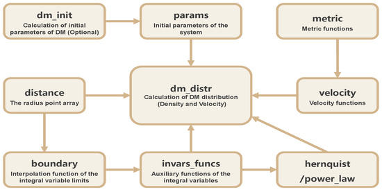
Figure 1. Package structure of DAMPS. Each box represents a module and describes its function. The arrows indicate the dependencies of the modules.

The params module serves as the central parameter configuration unit. All system parameters defined in the main program are passed to this module, which subsequently distributes them to other computational modules. For detailed parameter definitions and usage, please refer to the core function of the params module in Listing 1.

Listing 1. Core function of the params module for system parameter configuration.

The dm_init module, as shown in Listing 2, computes the parameters of the initial DM halo distribution based on the central black hole parameters provided in params. This module is optional, as the code supports two methods for defining the DM halo. The halo mass and scale radius (mhalo and r0) can be set directly in params. Alternatively, if these are not specified, the functions within dm_init can be called to derive them from the central black hole mass using a velocity dispersion relation.

Listing 2. Function of the dm_init module for calculating initial dark matter halo parameters.

The distance module determines the spatial sampling for the calculation by defining the minimum radius of DM particles and the radial grid points at which the density and velocity are evaluated.

As shown in Listing 3, the variable r_cutoff is implemented as an interpolation function. Within this module, a series of minimum orbital radii have been precomputed as functions of the black hole spin and the orbital inclination angle of the DM. For subsequent calculations, this interpolation function can be called directly to obtain the minimum radius for a given set of parameters. It is important to note that this procedure applies to the Kerr black hole scenario. For the Schwarzschild case, the minimum radius is simply set to the innermost stable circular orbit at $4G{M}_{\mathrm{BH}}$.

Listing 3. Functions of the distance module for radial grid generation and minimum radius interpolation.

The array of radial points used in the computation is constructed starting from this minimum radius. Since the method involves calculating DM density values at discrete radial points and then interpolating to obtain a continuous distribution, the selection of these points is critical. The returned variable r is a one-dimensional array containing these radial sample points. To enhance computational efficiency, this array can be partitioned for parallel processing in subsequent steps.

Notably, the radial points are sampled non-uniformly: a finer step size is used closer to the black hole, yielding a higher density of points, while a coarser sampling is adopted at larger radii. All these sampling parameters are user-configurable based on specific accuracy and performance requirements.

The metric module encapsulates the spacetime metric and associated expressions used in our calculations, including the individual metric components and auxiliary functions introduced to simplify the formalism. Since these metric-related functions are not directly invoked by the main computational workflow, they will not be discussed in further detail here. Interested readers may examine the corresponding source code for a complete implementation.

The velocity modulein Listing 4 defines the velocity component functions for DM particles. As seen in the function definitions, the magnitudes of individual velocity components as well as the resultant total velocity are each recorded.

Listing 4. Function of the velocity module for calculating dark matter particle velocity components.

The boundary module implements the computation of integration limits in the expression of the mass flow following the Jacobi transformation in Equation (4). It provides a function that calculates these integration boundaries, which is designed to be called directly by other modules in the package.

The function for solving the integral limits is defined in the initial part of this module, where a set of limits corresponding to various parameter values is precomputed. As illustrated in Listing 5, these precomputed values are used to construct an interpolation function, which is returned as the final implementation of the integral limit function. In subsequent computational steps, this interpolation function can be called directly to obtain the required integration limits.

Listing 5. Functions of the boundary module for interpolation of integral limits.

The invars_funcs module specifies the integration variables and auxiliary component functions appearing in the mass flow expression. It incorporates the integration limit function from the boundary module to supply the required boundary values for numerical evaluation. Several internal functions responsible for remapping integration variables are not directly invoked by the main workflow and are therefore omitted from this documentation.

The hernquist module implements the initial DM halo model based on the adiabatic invariant formulation corresponding to the Hernquist profile in Section 2.5. It provides the expression of the specific distribution function utilized in the calculation of the mass flow in Equation (4).

As these auxiliary functions in Listing 6 are not invoked by the main calculation and are stable, they are not detailed here but are available for inspection.

Listing 6. Functions of the hernquist module for adiabatic invariants and distribution function.

The power_law module, analogous to the hernquist module, implements the initial DM halo model using a single power-law distribution within the adiabatic invariant framework in Section 2.6. It supplies the corresponding distribution function expression for evaluation within the mass flow formalism in Equation (4).

The dm_distr module performs the core numerical computation. It implements a manual point-sampling procedure across different radial distances, applying the mirror-effective potential and angular-effective potential criteria to identify bound-orbit DM particles. The module subsequently calls functions from other modules to compute the corresponding density values at these validated positions.

The dm_distr module, as described in Listing 7, outputs the integrand values for the mass flow expression rather than the final DM density values. To derive the DM density profile, numerical integration of these outputs is required, a step implemented by the data_analyse module. This module generates DM density and velocity values at discrete radial points, and includes visualization examples that correspond to the DM figures presented in this paper.

Listing 7. Core function of the dm_distr module for dark matter density and velocity calculation.

Computational efficiency is enhanced via the implementation of task-level multi-process parallelism, which is realized by directly invoking the core computation function dm_rho_vel through Python’s built-in multiprocessing module. The key implementation steps are detailed as follows: first, the radial grid point array—used for evaluating DM density and particle velocities—is partitioned into non-overlapping subarrays using numpy.array_split, to facilitate task distribution across multiple processes; second, a process pool (multiprocessing.Pool) is initialized to allocate these subarrays to distinct CPU cores; finally, each CPU core executes dm_rho_vel in parallel, computing the DM density and particle velocities for its assigned subset of radial points. This parallelization scheme exploits multi-core hardware resources to enable simultaneous processing of independent radial grid point subsets, thereby shortening the overall computation time. The code snippet in Listing 8 illustrates the core workflow of this calculation:

Listing 8. Core computational workflow with multiprocessing parallelization.

4. Application

In this section, we use two DM profile examples to demonstrate the functionality of the code. We present the distribution characteristics of DM spikes at the center of the Milky Way black hole—using Hernquist and the single power-law profiles as the distribution functions of the initial dark halo, and using the distribution characteristics of DM to plot the GW waveforms corresponding to the extreme mass ratios close to binary stars.

We consider a black hole with a mass similar to M87, i.e., $M_{\mathrm{BH}}=6.5\times {10}^9{M}_{\odot }$. Since we are considering the Schwarzschild case, and the DM distribution inclination angle is $\theta =0$, corresponding to the DM distribution in the equatorial plane (the inclination has no effect in the Schwarzschild case). By invoking the rho_DM package, the initial distribution parameters for both the Hernquist profile and the single power-law profile can be computed from the black hole mass. Using the distance package, we define the radial range from $4G{M}_{\mathrm{BH}}$ to $100G{M}_{\mathrm{BH}}$. By calling the dm_distr package and processing the results with the data_analyse module, we obtain the corresponding density and velocity distributions of DM. For computational efficiency, we employ multiprocessing parallel computing, where the dm_distr function is invoked in parallel. The specific example code can be found in example_test.ipynb.

The results of the density distribution are shown in Figure 2. The blue dashed curve and red solid curve correspond to the post-accretion spike structures derived from the initial single power-law profile and the Hernquist profile, respectively. As we can see, both curves exhibit a typical spike feature in the logarithmic coordinate system, which is consistent with our expectations.

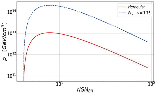
Figure 2. DM density profiles for two different initial halo profiles with $M_{\mathrm{BH}}=6.5\times {10}^9{M}_{\odot }$.

The density of DM up to a velocity v, $\rho \left(v\right)$, and the velocity distributions of the DM particles, $f\left(v\right)$, at different locations around the black hole are shown in Figure 3. The different curves in the figure correspond to the distributions in different r. Under the black hole mass considered of $M_{\mathrm{BH}}=6.5\times {10}^9{M}_{\odot }$, the corresponding total dark matter halo mass is $M_{\mathrm{halo}}=1.86\times {10}^{13}{M}_{\odot }$, yielding a mass ratio of $M_{\mathrm{BH}}/M_{\mathrm{halo}}=3.5\times {10}^{-4}$. According to the distant weak-field Newtonian analysis presented in [51], for this mass ratio and an initial Hernquist profile, the distribution function in the presence of a central black hole should exhibit minimal deviation from the black hole-free case, as indicated by Equation (16). Figure 3 displays the velocity distribution for an initial single power-law profile. Similarly, the velocity distribution curve can be plotted for dark matter particles with an initial Hernquist profile. Based on the definition of energy per unit mass $\mathcal{E}$ in Equation (3) and the velocity definition in Section 2.4, the velocity can be expressed in terms of $\mathcal{E}$ as $v=\sqrt{-g_{tt}-{\left(g_{tt}\right)}^2/{\mathcal{E}}^2}$, where $g_{tt}=-1+2G{M}_{\mathrm{BH}}/r$. Applying the Jacobi transformation to the dark matter particle velocity distribution $f(r,\alpha )$ to $f\left(\mathcal{E}\right)$, we can confirm that the distribution function at large distances aligns with the distant weak-field approximation. The impact of the central black hole on the distribution function is primarily concentrated in its immediate vicinity, consistent with conclusions regarding the central black hole’s influence on the dark matter halo density distribution.

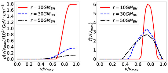
Figure 3. (Left panel) DM density up to a velocity v, $\rho \left(v\right)$, and (Right panel) velocity distribution of DM particles in the spike, $f\left(v\right)$, at different distances with $M_{\mathrm{BH}}=6.5\times {10}^9{M}_{\odot }$. The initial dark matter halo follows the power-law with $\gamma =1.75$.

Next, we can use the obtained DM halo density and velocity distributions, incorporate the DF of DM in the dynamics of EMRI evolution and calculate the corresponding GW waveform. We consider the secondary object in an EMRI binary both in vacuum and embedded the DM spike around the central primary black hole. We numerically evolve the orbital kinematic quantities of the secondary object using the geodesic Equation (11). However, considering the extremely high mass of the M87-like black hole, adopted in the preceding example, the evolution time of the corresponding EMRI system is prohibitively long—this property is suboptimal for illustrating the computational efficiency and practical applicability of our framework. We thus select instead a canonical EMRI system with mass parameters $(M,m)\sim ({10}^7{M}_{\odot },10M_{\odot })$, which aligns with the typical parameter range of EMRIs targeted by future space-based gravitational-wave detectors. For this canonical system, we recompute the dark matter density and velocity distributions around the central SMBH, where $M={10}^7{M}_{\odot }$, and further incorporate these updated distribution data into the subsequent gravitational-wave calculation, thereby ensuring the results better represent realistic observational scenarios.

The influences of the DF of DM spike on the evolution of energy E, angular momentum L, and GW radiation Q are given by

$$\begin{array}{c}\hfill {\displaystyle \frac{dE}{dt}}={\left({\displaystyle \frac{dE}{dt}}\right)}_{\mathrm{GW}}+{\left({\displaystyle \frac{dE}{dt}}\right)}_{\mathrm{DF}},{\displaystyle \frac{d{L}_z}{dt}}={\left({\displaystyle \frac{d{L}_z}{dt}}\right)}_{\mathrm{GW}}+{\left({\displaystyle \frac{d{L}_z}{dt}}\right)}_{\mathrm{DF}},{\displaystyle \frac{dQ}{dt}}={\left({\displaystyle \frac{dQ}{dt}}\right)}_{\mathrm{GW}}.\end{array}$$

(28)

The DF effect can be written as [41]

$$\begin{array}{cc}\hfill {\left({\displaystyle \frac{dE}{dt}}\right)}_{\mathrm{DF}}& ={\widehat{F}}_{\mathrm{DF}}·\widehat{v}=-{\displaystyle \frac{4\pi \rho (r,<v)G^2{m}^2{\gamma }^2{\left[1+{(v/c)}^2\right]}^2}{v}}ln\mathsf{\Lambda },\hfill \\ \hfill {\left({\displaystyle \frac{d{L}_z}{dt}}\right)}_{\mathrm{DF}}& =r·{\widehat{F}}_{\mathrm{DF}}{\displaystyle \frac{r\dot{\psi }}{v}}=-{\displaystyle \frac{4\pi \rho (r,<v)G^2{m}^2{r}^2\dot{\psi }{\gamma }^2{\left[1+{(v/c)}^2\right]}^2}{v^2}}ln\mathsf{\Lambda },\hfill \end{array}$$

(29)

where $\gamma ={\displaystyle \frac{1}{\sqrt{1-{(v/c)}^2}}}$, and $ln\mathsf{\Lambda }=10$. The density term $\rho (r,<v)$ in the DF formula is given by interpolation of DM density and velocity output by our code. The gravitational radiation term is given by the post-Newtonian formalism. We take the 3PN term into account [52]:

$$\begin{array}{cc}\hfill {\left({\displaystyle \frac{dE}{dt}}\right)}_{GW}& =f_E(a,M,m,p,e,\iota ),\hfill \\ \hfill {\left({\displaystyle \frac{d{L}_z}{dt}}\right)}_{GW}& =f_L(a,M,m,p,e,\iota ),\hfill \\ \hfill {\left({\displaystyle \frac{dQ}{dt}}\right)}_{GW}& =f_Q(a,M,m,p,e,\iota ),\hfill \end{array}$$

(30)

where ${tan}^2\iota ={\displaystyle \frac{Q}{L_z^2}}$, $f_E,f_L,f_Q$ are post-Newton’s formulas.

Subsequently, we can obtain all the temporal kinematic quantities of EMRI system through numerical evolution, and the corresponding GW waveform in time domain can be obtained by substituting the quadrupole–octupole formula [53]:

$$\begin{array}{c}\hfill h_{jk}(t,\overrightarrow{x})={\displaystyle \frac{2}{r}}\left[{\ddot{I}}_{jk}-2n_i{\ddot{S}}_{ijk}+n_i{\ddot{M}}_{ijk}\right]{|}_{t^{\prime }=t-{\displaystyle \frac{d}{c}}},\end{array}$$

(31)

where an overdot denotes a time-derivative, d is the distance from the source to detector, and $n_i$ are the components of direction vector $\widehat{n}=\widehat{d}/d=(sin{\theta }_{D}cos{\varphi }_D,sin{\theta }_{D}sin{\varphi }_D,cos{\varphi }_D)$, specified by the azimuth ${\varphi }_D$ and latitude ${\theta }_D$ of the source in the sky. And the multipole moments are

$$\begin{array}{c}\hfill I_{jk}=m{x}_j{x}_k,S_{ijk}=m{v}_i{x}_j{x}_k,M_{ijk}=m{x}_i{x}_j{x}_k.\end{array}$$

(32)

Herein, we neglect time-dependent mass growth of both the central black hole and the secondary black hole in the EMRI system. This neglect is supported by results from [54], which demonstrate that the effects induced by such black hole mass growth are negligible for orbital dynamics calculations and GW waveform modeling—specifically, these mass changes do not introduce measurable perturbations to orbital parameters or the evolution of the GW phase.

Figure 4 illustrates the impact of DM-induced DF on the GW waveforms of EMRIs. A key observation from the figure is that the waveform incorporating DM-induced DF exhibits a phase deviation relative to the DF-free counterpart. This phase discrepancy does not remain constant but accumulates gradually as the inspiral progresses, becoming increasingly pronounced in the late evolutionary stage. While we cannot directly observe the rate of this phase deviation accumulation from the waveform itself, we can anticipate that this accumulation rate inevitably slows as the inspiral advances—this is because the DM density drops sharply as the secondary black hole approaches the central SMBH, and the strength of DM-induced DF is closely dependent on the local DM density, leading to a reduced rate of additional phase accumulation in later stages. The amplified views of critical inspiral phases further confirm that the deviation is not a localized artifact but a systematic shift driven by DM-DF effects, which modulates the inspiral trajectory and thus the gravitational-wave phase evolution. This result highlights the non-negligible role of DM spikes in shaping EMRI gravitational-wave signals, providing a potential avenue for constraining DM halo properties through future gravitational-wave detections.

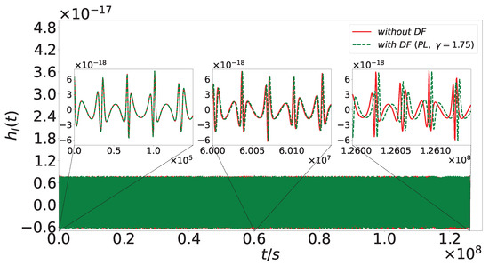
Figure 4. Gravitational-wave waveforms of EMRIs with $(M,m)\sim ({10}^7{M}_{\odot },10M_{\odot })$ under two scenarios: the solid red curve represents the case without dark matter-induced DF, while the dashed green curve corresponds to the case with DF (adopting a power-law initial DM halo profile with slope $\gamma =1.75$). The large green area at the bottom displays the full-duration waveform, while the three inset panels present magnified details of the waveform at the early, middle, and late phases within the observed time window, respectively.

5. Summary

The density and velocity distributions of dark matter around massive black holes can play an important role in the binary dynamics and gravitational-wave physics. Here, we have introduced a comprehensive computational framework for determining the relativistic density and velocity distributions of DM spikes around SMBHs. We have detailed the theoretical foundation underlying the code, explained its modular structure, and demonstrated its application through two representative examples using Hernquist and single power-law initial DM profiles. Furthermore, we have illustrated how the output of the code can be utilized to study the impact of DM-induced DF on the GW signals from EMRIs.

The presented package provides a practical tool for quantifying DM spike properties, thereby bridging theoretical halo models and gravitational-wave astrophysics. While the current version focuses on Schwarzschild black holes, the underlying formalism is extensible to the Kerr metric, a planned enhancement for future releases. We anticipate that this tool will support the community in preparing for and interpreting observations from future space-based gravitational-wave detectors by enabling detailed studies of environmental effects, particularly those related to dark matter, around massive black holes.

References

- Andernach, H.; Zwicky, F. English and Spanish translation of Zwicky’s (1933) the redshift of extragalactic nebulae. arXiv 2017, arXiv:1711.01693. [Google Scholar]
- Rubin, V.C.; Ford, W.K., Jr. Rotation of the Andromeda Nebula from a Spectroscopic Survey of Emission Regions. Astrophys. J. 1970, 159, 379. [Google Scholar] [CrossRef]
- Tyson, J.A.; Kochanski, G.P.; Dell’Antonio, I.P. Detailed mass map of CL 0024+1654 from strong lensing. Astrophys. J. 1998, 498, L107–L110. [Google Scholar] [CrossRef]
- Refregier, A. Weak gravitational lensing by large-scale structure. Annu. Rev. Astron. Astrophys. 2003, 41, 645–668. [Google Scholar] [CrossRef]
- Clowe, D.; Bradač, M.; Gonzalez, A.H.; Markevitch, M.; Randall, S.W.; Jones, C.; Zaritsky, D. A Direct Empirical Proof of the Existence of Dark Matter. Astrophys. J. Lett. 2006, 648, L109–L113. [Google Scholar] [CrossRef]
- Akerib, S. et al. [LUX Collaboration] Results from a Search for Dark Matter in the Complete LUX Exposure. Phys. Rev. Lett. 2017, 118, 021303. [Google Scholar] [CrossRef]
- Meng, Y. et al. [PandaX-4T Collaboration] Dark Matter Search Results from the PandaX-4T Commissioning Run. Phys. Rev. Lett. 2021, 127, 261802. [Google Scholar] [CrossRef]
- Aprile, E. et al. [XENON Collaboration] XENONnT WIMP Search: Signal and Background Modeling and Statistical Inference. Phys. Rev. D 2025, 111, 103040. [Google Scholar] [CrossRef]
- Liang, Y.F. et al. [CDEX Collaboration] Constraints on Inelastic Dark Matter from the CDEX-1B Experiment. arXiv 2025, arXiv:2510.07800. [Google Scholar] [CrossRef]
- Ibarra, A.; Tran, D.; Weniger, C. Indirect searches for decaying dark matter. Int. J. Mod. Phys. 2013, 28, 1330040. [Google Scholar] [CrossRef]
- Donato, F. Indirect searches for dark matter. Phys. Dark Universe 2014, 4, 41–43. [Google Scholar] [CrossRef]
- Buchmueller, O.; Doglioni, C.; Wang, L.-T. Search for dark matter at colliders. Nat. Phys. 2017, 13, 217–223. [Google Scholar] [CrossRef]
- Cole, P.S.; Bertone, G.; Coogan, A.; Gaggero, D.; Karydas, T.K.; Kavanagh, B.J.; Spieksma, T.F.M.; Tomaselli, G.M. Distinguishing environmental effects on binary black hole gravitational waveforms. Nat. Astron. 2023, 7, 943–950. [Google Scholar] [CrossRef]
- Kavanagh, B.J.; Nichols, D.A.; Bertone, G.; Gaggero, D. Detecting dark matter around black holes with gravitational waves: Effects of dark-matter dynamics on the gravitational waveform. Phys. Rev. D 2020, 102, 083006. [Google Scholar] [CrossRef]
- Eda, K.; Itoh, Y.; Kuroyanagi, S.; Silk, J. New probe of dark-matter properties: Gravitational waves from an intermediate-mass black hole embedded in a dark-matter minispike. Phys. Rev. Lett. 2013, 110, 221101. [Google Scholar] [CrossRef]
- Bertone, G.; Croon, D.; Amin, M.A.; Boddy, K.K.; Kavanagh, B.J.; Mack, K.J.; Natarajan, P.; Opferkuch, T.; Schutz, K.; Takhistov, V.; et al. Gravitational wave probes of dark matter: Challenges and opportunities. SciPost Phys. Core 2020, 3, 007. [Google Scholar] [CrossRef]
- Coogan, A.; Bertone, G.; Gaggero, D.; Kavanagh, B.J.; Nichols, D.A. Measuring the dark matter environments of black hole binaries with gravitational waves. Phys. Rev. D 2022, 105, 043009. [Google Scholar] [CrossRef]
- Amaro-Seoane, P.; Audley, H.; Babak, S.; Baker, J.; Barausse, E.; Bender, P.; Berti, E.; Binetruy, P.; Born, M.; Bortoluzzi, D.; et al. Laser Interferometer Space Antenna. arXiv 2017, arXiv:1702.00786. [Google Scholar] [CrossRef]
- Hu, W.-R.; Wu, Y.-L. The Taiji Program in Space for gravitational wave physics and the nature of gravity. Natl. Sci. Rev. 2017, 4, 685–686. [Google Scholar] [CrossRef]
- Luo, J.; Chen, L.-S.; Duan, H.; Gong, Y.-G.; Hu, S.; Ji, J.; Liu, Q.; Mei, J.; Milyukov, V.; Sazhin, M. Tianqin: A space-borne gravitational wave detector. Class. Quantum Gravity 2016, 33, 035010. [Google Scholar] [CrossRef]
- Kawamura, S.; Ando, M.; Seto, N.; Sato, S.; Musha, M.; Kawano, I.; Yokoyama, J.; Tanaka, T.; Ioka, K.; Akutsu, T.; et al. Current status of space gravitational wave antenna DECIGO and B-DECIGO. Prog. Theor. Exp. Phys. 2021, 2021, 05A105. [Google Scholar] [CrossRef]
- Mukherjee, D.; Holgado, A.M.; Ogiya, G.; Trac, H. Examining the effects of dark matter spikes on eccentric intermediate mass ratio inspirals using n-body simulations. Mon. Not. R. Astron. Soc. 2024, 533, 2335–2355. [Google Scholar] [CrossRef]
- Einasto, J. On the Construction of a Composite Model for the Galaxy and on the Determination of the System of Galactic Parameters. Tr. Astrofiz. Instituta-Alma-Ata 1965, 5, 87–100. [Google Scholar]
- Hernquist, L. An Analytical Model for Spherical Galaxies and Bulges. Astrophys. J. 1990, 356, 359. [Google Scholar] [CrossRef]
- Navarro, J.F.; Frenk, C.S.; White, S.D.M. The Structure of Cold Dark Matter Halos. Astrophys. J. 1996, 462, 563. [Google Scholar] [CrossRef]
- Navarro, J.F.; Frenk, C.S.; White, S.D.M. A universal density profile from hierarchical clustering. Astrophys. J. 1997, 490, 493. [Google Scholar] [CrossRef]
- Gondolo, P.; Silk, J. Dark matter annihilation at the galactic center. Phys. Rev. Lett. 1999, 83, 1719–1722. [Google Scholar] [CrossRef]
- Sadeghian, L.; Ferrer, F.; Will, C.M. Dark-matter distributions around massive black holes: A general relativistic analysis. Phys. Rev. D 2013, 88, 063522. [Google Scholar] [CrossRef]
- Ferrer, F.; da Rosa, A.M.; Will, C.M. Dark matter spikes in the vicinity of Kerr black holes. Phys. Rev. D 2017, 96, 083014. [Google Scholar] [CrossRef]
- Bergström, L.; Ullio, P.; Buckley, J.H. Observability of γ rays from dark matter neutralino annihilations in the milky way halo. Astropart. Phys. 1998, 9, 137–162. [Google Scholar] [CrossRef]
- Buckley, J.; Cowen, D.F.; Profumo, S.; Archer, A.; Cahill-Rowley, M.; Cotta, R.; Digel, S.; Drlica-Wagner, A.; Ferrer, F.; Funk, S.; et al. Cosmic frontier indirect dark matter detection working group summary. arXiv 2013, arXiv:1310.7040. [Google Scholar] [CrossRef]
- Ackermann, M. et al. [The Fermi LAT Collaboration] The Fermi galactic center gev excess and implications for dark matter. Astrophys. J. 2017, 840, 43. [Google Scholar] [CrossRef]
- Lacroix, T.; Stref, M.; Lavalle, J. Anatomy of Eddington-like inversion methods in the context of dark matter searches. J. Cosmol. Astropart. Phys. 2018, 2018, 040. [Google Scholar] [CrossRef]
- Xie, Z.-M.; Yuan, H.-C.; Tang, Y. On Equation of State of Dark Matter around Massive Black Holes. Sci. China Phys. Mech. Astron. 2025, 69, 210412. [Google Scholar] [CrossRef]
- Antonini, F.; Merritt, D. Dynamical friction around supermassive black holes. Astrophys. J. 2011, 745, 83. [Google Scholar] [CrossRef]
- Chan, M.H.; Lee, C.M. Indirect evidence for dark matter density spikes around stellar-mass black holes. Astrophys. J. Lett. 2023, 943, L11. [Google Scholar] [CrossRef]
- Chan, M.H.; Lee, C.M. The first robust evidence showing a dark matter density spike around the supermassive black hole in oj 287. Astrophys. J. Lett. 2024, 962, L40. [Google Scholar] [CrossRef]
- Chandrasekhar, S. Dynamical Friction. I. General Considerations: The Coefficient of Dynamical Friction. Astrophys. J. 1943, 97, 255. [Google Scholar] [CrossRef]
- Yue, X.-J.; Han, W.-B.; Chen, X. Dark matter: An efficient catalyst for intermediate-mass-ratio-inspiral events. Astrophys. J. 2019, 874, 34. [Google Scholar] [CrossRef]
- Fakhry, S.; Salehnia, Z.; Shirmohammadi, A.; Yengejeh, M.G.; Firouzjaee, J.T. Compact binary merger rate in dark-matter spikes. Astrophys. J. 2023, 947, 46. [Google Scholar] [CrossRef]
- Becker, N.; Sagunski, L.; Prinz, L.; Rastgo, S.o. Circularization versus eccentrification in intermediate mass ratio inspirals inside dark matter spikes. Phys. Rev. 2022, 105, 063029. [Google Scholar] [CrossRef]
- Li, G.-L.; Tang, Y.; Wu, Y.-L. Probing dark matter spikes via gravitational waves of extreme-mass-ratio inspirals. Sci. China Phys. Mech. Astron. 2022, 65, 100412. [Google Scholar] [CrossRef]
- Zhang, Z.-C.; Tang, Y. Velocity distribution of dark matter in spikes around Schwarzschild black holes and effects on gravitational waves from extreme-mass-ratio inspirals. Phys. Rev. D 2024, 110, 103008. [Google Scholar] [CrossRef]
- Zhang, Z.-C.; Yuan, H.-C.; Tang, Y. Universal density and velocity distributions of dark matter around massive black holes. Phys. Rev. D 2025, 112, 043025. [Google Scholar] [CrossRef]
- Ullio, P.; Zhao, H.; Kamionkowski, M. Dark-matter spike at the galactic center? Phys. Rev. D 2001, 64, 043504. [Google Scholar] [CrossRef]
- Ferrarese, L.; Merritt, D. A fundamental relation between supermassive black holes and their host galaxies. Astrophys. J. 2000, 539, L9. [Google Scholar] [CrossRef]
- Gebhardt, K.; Bender, R.; Bower, G.; Dressler, A.; Faber, S.M.; Filippenko, A.V.; Green, R.; Grillmair, C.; Ho, L.C.; Kormendy, J.; et al. A relationship between nuclear black hole mass and galaxy velocity dispersion. Astrophys. J. 2000, 539, L13. [Google Scholar] [CrossRef]
- Hannuksela, O.A.; Ng, K.C.Y.; Li, T.G.F. Extreme dark matter tests with extreme mass ratio inspirals. Phys. Rev. D 2020, 102, 103022. [Google Scholar] [CrossRef]
- Nishikawa, H.; Kovetz, E.D.; Kamionkowski, M.; Silk, J. Primordial-black-hole mergers in dark-matter spikes. Phys. Rev. D 2019, 99, 043533. [Google Scholar] [CrossRef]
- Sánchez-Conde, M.A.; Prada, F. The Flattening of the Concentration–Mass Relation Towards Low Halo Masses and Its Implications for the Annihilation Signal Boost. Mon. Not. R. Astron. Soc. 2014, 442, 2271–2277. [Google Scholar] [CrossRef]
- Tremaine, S.; Richstone, D.O.; Byun, Y.I.; Dressler, A.; Faber, S.M.; Grillmair, C.; Kormendy, J.; Lauer, T.R. A family of models for spherical stellar systems. AJ 1994, 107, 634. [Google Scholar] [CrossRef]
- Sago, N.; Fujita, R. Calculation of radiation reaction effect on orbital parameters in Kerr spacetime. Prog. Theor. Exp. Phys. 2015, 2015, 073E03. [Google Scholar] [CrossRef]
- Babak, S.; Fang, H.; Gair, J.R.; Glampedakis, K.; Hughes, S.A. “Kludge” gravitational waveforms for a test-body orbiting a Kerr black hole. Phys. Rev. 2007, 75, 024005. [Google Scholar] [CrossRef]
- Karydas, T.K.; Kavanagh, B.J.; Bertone, G. Sharpening the Dark Matter Signature in Gravitational Waveforms. I. Accretion and Eccentricity Evolution. Phys. Rev. D 2025, 111, 063070. [Google Scholar] [CrossRef]
- Harris, C.R.; Millman, K.J.; van der Walt, S.J.; Gommers, R.; Virtanen, P.; Cournapeau, D.; Wieser, E.; Taylor, J.; Berg, S.; Smith, N.J.; et al. Array Programming with NumPy. Nature 2020, 585, 357–362. [Google Scholar] [CrossRef]
- Virtanen, P.; Gommers, R.; Oliphant, T.E.; Haberland, M.; Reddy, T.; Cournapeau, D.; Burovski, E.; Peterson, P.; Weckesser, W.; Bright, J.; et al. SciPy 1.0: Fundamental Algorithms for Scientific Computing in Python. Nat. Methods 2020, 17, 261–272. [Google Scholar] [CrossRef] [PubMed]
- Hunter, J.D. Matplotlib: A 2D Graphics Environment. Comput. Sci. Eng. 2007, 9, 90–95. [Google Scholar] [CrossRef]
Disclaimer/Publisher’s Note: The statements, opinions and data contained in all publications are solely those of the individual author(s) and contributor(s) and not of MDPI and/or the editor(s). MDPI and/or the editor(s) disclaim responsibility for any injury to people or property resulting from any ideas, methods, instructions or products referred to in the content. |
© 2025 by the authors. Licensee MDPI, Basel, Switzerland. This article is an open access article distributed under the terms and conditions of the Creative Commons Attribution (CC BY) license (https://creativecommons.org/licenses/by/4.0/).