Model Identification and Trajectory Tracking Control for Vector Propulsion Unmanned Surface Vehicles

Abstract

To promote the development of military and civilian applications for marine technology, more and more scientific research around the world has begun to develop unmanned surface vehicles (USVs) technology with advanced control capabilities. This paper establishes and identifies the model of vector propulsion USV, which is widely used at present. After analyzing its actuator distribution, we consider that the more realistic vessel model should be an incomplete underactuated system. For this system, a virtual control point method is adopted and an adaptive sliding mode trajectory tracking controller with neural network minimum learning parameter (NNMLP) theory is designed. Finally, in the simulation experiment, the thruster speed and propulsion angle are used as the inputs of the controller, and the linear and circular trajectory tracking tests are carried out considering the delay effect of the actuator, system uncertainty, and external disturbance. The results show that the proposed tracking control framework is reasonable.

1. Introduction

Due to the superior performance of unmanned surface vehicles (USVs) in terms of economy and strategically, the number of USVs used for various missions is increasing globally [1,2]. To accomplish the task efficiently in the complex marine environment, both the propulsion system and autonomous control system of USV need continuous improvement [3]. In the aspect of propulsion system, a vector propulsion equipment was put forward, which is superior to the traditional propeller-rudder propulsion system in propulsion efficiency [4,5]. For the autonomous control system, trajectory tracking control is a very important research topic, and this paper needs to consider how to design the controller based on the vector propulsion system.

For the USV with a vector propulsion device, it is necessary to analyze and identify its mathematical model. Since 1964, more and more attention has been paid to the study of vessel models [6]. In the process of research, it is divided into two kinds of modeling methods, one is the holistic model, which belongs to a semi-theoretical and semi-empirical model pattern, represented by Abokowitz’s [6] and Norrbin’s [7] non-linear ship mathematical models; and the other is a separation motion mathematical model proposed by the Maneuvering Modeling Group (MMG), which has complete theoretical support [8]. In 2015, a new standardization study about MMG was carried out by the Japan Society of Naval Architects and Ocean Engineers [9]. In this paper, the mathematical model of USV adopts the MMG modeling theory. The existing ship models are all based on the traditional propulsion system with propeller-rudder separation, while the research on the ship model with vector propulsion is less concerned. Vector propulsion includes POD and waterjet propulsion, among which POD propulsion is a common propulsion mode. At present, the research on vector propulsion system mainly focuses on hydrodynamic performance, such as Literature [10,11,12]. For the research of the ship manoeuvre model with vector propulsion, Gierusz compared vector propulsion system with traditional propulsion system from the point of future control applications [5], and studied the forces generated [13] and full model [14] with two podded thrusters of LNG carrier. In [15], based on the MMG method, a motion mathematical model of a 10,000 DWT pod-driven coastal tanker is established, and the description of vector driving force is given. However, both of the above studies are to model large ships with dual POD propulsion. Mu et al. [16] studied the model establishment of USV driven by single vector propulsion system based on MMG theory, but neglected the influence of sway motion force and simplified it to traditional ship model. This paper mainly studies the manoeuvring model of a small USV with single vector propulsion to provide a basis for the research of trajectory tracking controller.

In recent years, with the continuous improvement of the nonholonomic system theory, the problem of actuator constraints and effectiveness faults [17] and underactuated tracking [18,19,20] of ships have also been actively studied. In this paper, the effect of sway thrust is very obvious for small USV with vector propulsion when the output is selected at the geometric center of the vessel. In addition, such an incomplete underactuated system is accompanied by unstable internal dynamics [21]. Current research on ship tracking control usually neglects the sway thrust [3], but there are still some papers trying to solve this kind of incomplete underactuated system. Toussaint et al. explained the selection of the output when the generalized forces act on the vessel, and used the backstepping method to design the controller for trajectory tracking [22]. On this basis, the state estimator was used to deal with the uncertainty of state measurement [23]. However, they need noncausal dynamic inversion to find the reference trajectory.

In this paper, the research object is the vector propulsion USV. The vector propulsion system can carry out full speed propulsion in any direction within the range of the propulsion angle, so as to generate large sway force that is difficult to be ignored, which makes the difference between the vector propulsion ship model and the underactuated ship model. In the research of traditional underactuated ship tracking control, the influence of sway force is generally ignored, because the propeller of traditional propeller-rudder propulsion system is fixed and the hydrodynamic force of rudder surface only produces small sway force [3]. For the vector propulsion USV, the main contribution of the paper can be summed up as that, firstly, the three degree-of-freedom (3-DOF) mathematical model of vector propulsion USV is obtained by analyzing the force distribution, and its model parameters are identified through field experiments, which provides a reference for the design of the controller; secondly, the method of virtual control point is used to solve the incomplete underactuated system; finally, an adaptive sliding mode controller based on neural network minimum learning parameter (NNMLP) is designed with disturbances and uncertainties. The robustness of this controller is tested by simulation in four cases with more practical control inputs.

The rest of this paper is organized as follows. In Section 2, the mathematical model of vector propulsion USV is established and its parameters are identified. Section 3 describes the trajectory tracking control laws based on virtual control point method and neural network minimum learning parameter, and the stability analysis is introduced in Section 4. Section 5 simulates and verifies the designed controller. Finally, the paper is discussed and summarized in Section 6.

2. USV Modeling and Identification

2.1. Lanxin USV with Vector Propulsion

Lanxin USV is a small intelligent marine vessel of Dalian Maritime University with length $L=$ 7.02 m [24]. It mainly consists of vector propulsion system, NGC (navigation, guidance and control) system, sensing system and communication system. Its appearance is shown in Figure 1.

The propulsion system of the USV adopts vector propulsion, as shown in Figure 2. The maximum output power of this system can reach to 260 HP. Its thruster is composed of three leaf propeller with a diameter of 0.46 meter. The maximum thrust can be achieved in any direction within the propulsion angle range ($-{30}^{\circ }$∼$+{30}^{\circ }$) [25].

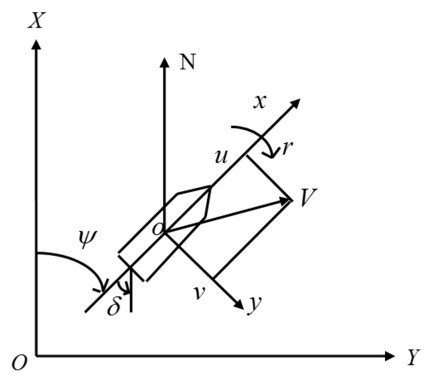
2.2. Mathematical Model of the USV

For vector propulsion USV, the description of plane motion variables is shown in Figure 3.

The kinematics and dynamics equations of the marine surface vessel can be expressed as [26,27]

$$\begin{array}{c}\hfill \left\{\begin{array}{c}\dot{x}=ucos\psi -vsin\psi \hfill \\ \dot{y}=usin\psi +vcos\psi \hfill \\ \dot{\psi }=r\hfill \\ \dot{u}=f_u+{\mathsf{\Delta }}_u+\frac{1}{m_{11}}({\tau }_u+b_u)\hfill \\ \dot{v}=f_v+{\mathsf{\Delta }}_v+\frac{1}{m_{22}}({\tau }_v+b_v)\hfill \\ \dot{r}=f_r+{\mathsf{\Delta }}_r+\frac{1}{m_{33}}({\tau }_r+b_r)\hfill \end{array}\right.,\end{array}$$

(1)

with

$$\begin{array}{c}\hfill \begin{array}{c}{f}_u=\frac{m_{22}}{m_{11}}vr-\frac{d_{11}}{m_{11}}u\hfill \\ f_v=-\frac{m_{11}}{m_{22}}ur-\frac{d_{22}}{m_{22}}v\hfill \\ f_r=\frac{m_{11}-m_{22}}{m_{33}}uv-\frac{d_{33}}{m_{33}}r\hfill \end{array},\end{array}$$

where $(x,y,\psi )$ are the surge, sway displacement and yaw angle in the earth fixed coordinate system, $(u,v,r)$ and $({\tau }_u,{\tau }_v,{\tau }_r)$ denote the surge, sway, and yaw velocities and thrust (moment) components. Parameters $m_{ii}$ and $d_{ii}$ are given by the vessel inertia and damping matrices. $({\mathsf{\Delta }}_u,{\mathsf{\Delta }}_v,{\mathsf{\Delta }}_r)$ and $(b_u,b_v,b_r)$ denote the unmodeled dynamics and immeasurable external disturbances in each direction. The force distribution of vector propulsion USV is as follows [13,21]

$$\begin{array}{c}\hfill \begin{array}{c}\left\{\begin{array}{c}{\tau }_u=Tcos\left(\delta \right)\hfill \\ {\tau }_v=-Tsin\left(\delta \right)\hfill \\ {\tau }_r=Tsin\left(\delta \right)L/2\hfill \end{array}\right.\hfill \\ T=\left(1-t_p\right)\rho n^2{D}_p^4{K}_T\hfill \end{array},\end{array}$$

(2)

where T is the thrust of propulsion system, vector propulsion angle $\delta$ and thruster speed n are generated by vector propulsion system as control inputs [28], which can be obtained by

$$\begin{array}{c}\hfill \left\{\begin{array}{c}\delta =arctan\left(\frac{2{\tau }_r}{{\tau }_{u}L}\right)\hfill \\ n=\sqrt{\frac{{\tau }_u}{\left(1-t_p\right)\rho D_p^4{K}_{T}cos\left(\delta \right)}}\hfill \end{array}\right..\end{array}$$

(3)

The first-order and the second-order system are used as the response models of the actuator including the thruster speed and propulsion angle. The permissible ranges of thruster speed and propulsion angle are $n\in [0,n_{max}]$ and $\delta \in [-{\delta }_m,{\delta }_m]$.

2.3. Model Identification

Before model identification, field experiments including zig-zag test and turning test are needed to collect identification data. To reduce the external disturbances, it is necessary to ensure the relative stability of the marine environment during the experiments.

The collected data in the field experiments include vessel status data ($x,y,\psi ,u,v,r$) and vessel maneuvering control data ($\delta ,n$). The model parameters are identified by multiple-input multiple-output recursive least squares (MIMO-RLS) method [29,30], which needs to transformed the transfer function matrix model with r inputs and m outputs into

$$\begin{array}{lll}G\left(z\right)& =& \frac{\mathbf{B}\left(z^{-1}\right)}{A\left(z^{-1}\right)}\\ & =& \frac{1}{A\left(z^{-1}\right)}\left[\begin{array}{ccc}{B}_{11}\left(z^{-1}\right)& \cdots & B_{1r}\left(z^{-1}\right)\\ ⋮& \ddots & ⋮\\ B_{m1}\left(z^{-1}\right)& \cdots & B_{mr}\left(z^{-1}\right)\end{array}\right],\end{array}$$

(4)

with

$$\begin{array}{c}\hfill \left\{\begin{array}{c}A\left(z^{-1}\right)=1+a\left(1\right)z^{-1}+a\left(2\right)z^{-2}+\cdots +a\left(n_a\right)z^{-n_a}\hfill \\ B_{ij}\left(z^{-1}\right)=z^{-d_{ij}}\left[b_{ij}\left(0\right)+b_{ij}\left(1\right)z^{-1}+\cdots +b_{ij}\left(n_{bij}\right)z^{-n_{bij}}\right]\hfill \\ i=1,2,\cdots ,m;j=1,2,\cdots ,r\hfill \end{array}\right..\end{array}$$

According to Equation (4), the vessel model can be transformed. Taking the third equation of (1) as an example, the transformation matrix Equation (5) can be obtained with step h.

$$\begin{array}{c}\hfill r\left(k\right)=\frac{\left[\frac{m_{11}-m_{22}}{m_{33}}h{z}^{-1}\frac{1}{m_{33}}h{z}^{-1}\right]·\left[\begin{array}{c}uv\left(k\right)\hfill \\ {\tau }_r\left(k\right)\hfill \end{array}\right]}{1+(\frac{d_{33}}{m_{33}}h-1)z^{-1}}.\end{array}$$

(5)

Considering that zig-zag test requires constant change of propulsion angle, which can fully reflect the vessel’s maneuverability, the identification data mainly come from ${10}^{\circ }/{10}^{\circ }$ zig-zag test, and the ${10}^{\circ }$ turning test is used as a further verification test. The final identification result is: $m_{11}=2652.25$, $m_{22}=2825.29$, $m_{33}=4201.26$, $d_{11}=848.05$, $d_{22}=10161.62$, $d_{33}=22719.39$.

The propulsion angle response model is identified by ordinary RLS as a second-order system with the command propulsion angle $\delta$ as input and actual propulsion angle ${\delta }_r$ as output [31,32]. Finally, its identification parameters are the natural frequency ${\omega }_n=2.84$, damping ratio $\zeta =1.53$, and proportionality coefficient $K=1.02$.

2.4. Model Validation

The identified model are simulated and compared with the field experiments results to determine the feasibility of identification results. For ${10}^{\circ }/{10}^{\circ }$ zig-zag test, Figure 4a shows the comparison results of command propulsion angle $\delta$, actual propulsion angle ${\delta }_r$, and heading angle $\psi$. After the first period, the errors of heading angle and steering cycles are less than $2^{\circ }$ and 0.5 s respectively. In Figure 4b, the vessel’s actual and simulated ${10}^{\circ }$ turning trajectories are compared and their turning diameters are 79.94 m and 78.03 m. Because the tested USV is a small vessel with the length of 7.02 m, although it was tested in a stable sea condition as far as possible, it is still affected by the disturbances of external environment. Therefore, it is reasonable that there is a small error between the identification and experiment results, but this error will accumulate with time, as shown in Figure 4a, there is a large phase difference between the simulation and actual data in the later stage. In Figure 4b, to make the comparison between the simulation and actual trajectories more intuitive, the simulation trajectory is translated to the position where it coincides with the actual trajectory. It can be seen from Figure 4b that the two trajectories roughly coincide, and the reason for the actual trajectory to produce the transverse movement is that the USV is inevitably affected by the disturbances of the current and so on during the field experiments.

Next, the correctness of the model parameters is further verified by the state quantities. In Figure 5, the vessel’s state quantities $(u,v,r)$ are compared, and the surge velocity u and yaw rate r are basically the same. The sway velocity v deviates greatly due to external disturbances, but the change trend is basically the same. It can be seen that the simulation results are close to the actual test results, so the identified parameters are available.

3. Trajectory Tracking Controller

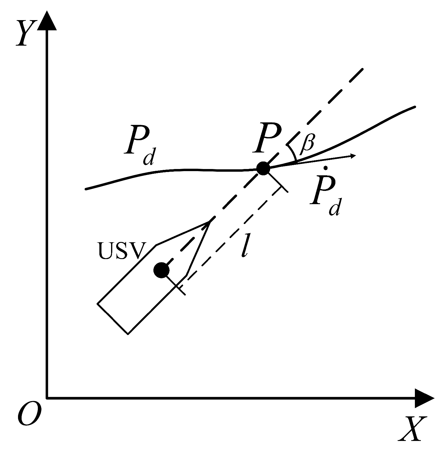
3.1. Preliminaries

The dynamics Equation (1) of the vessel along (2) can be re-expressed as

$$\left\{\begin{array}{c}\dot{u}=f_u+\frac{1}{m_{11}}{\tau }_u+d_u\hfill \\ \dot{v}=f_v-\frac{\partial }{m_{22}}{\tau }_r+d_v\hfill \\ \dot{r}=f_r+\frac{1}{m_{33}}{\tau }_r+d_r\hfill \end{array}\right.,$$

(6)

with $\partial =2/L$, and the disturbances terms d in each direction including the $\mathsf{\Delta }$ and b are $d_u={\mathsf{\Delta }}_u+\frac{1}{m_{11}}{b}_u$, $d_v={\mathsf{\Delta }}_v+\frac{1}{m_{22}}{b}_v$, $d_r={\mathsf{\Delta }}_r+\frac{1}{m_{33}}{b}_r$.

• Remark 1: There are unknown positive constants ${\overline{d}}_u$, ${\overline{d}}_v$, ${\overline{d}}_r$, so the d satisfies $\left|d_u\right|\le {\overline{d}}_u$, $\left|d_v\right|\le {\overline{d}}_v$, $\left|d_r\right|\le {\overline{d}}_r$.

The model (6) is an incomplete underactuated system with unstable internal dynamics [21,33]. This paper introduces virtual control point P to solve this problem, as shown in Figure 6. In addition, the distance from point P to the vessel center is $l>0$ with the reference trajectory $P_d={\left[x_d\left(t\right),y_d\left(t\right)\right]}^T$. So point P is

$$P=\left[\begin{array}{c}{x}_p\left(t\right)\\ y_p\left(t\right)\end{array}\right]=\left[\begin{array}{c}x\left(t\right)\\ y\left(t\right)\end{array}\right]+l\left[\begin{array}{c}cos\psi \left(t\right)\\ sin\psi \left(t\right)\end{array}\right].$$

(7)

• Remark 2: The reference trajectory $P_d$ requires sufficient smoothness, i.e., $x_{pd}$, ${\dot{x}}_{pd}$, ${\ddot{x}}_{pd}$, $y_{pd}$, ${\dot{y}}_{pd}$, ${\ddot{y}}_{pd}$ are all bounded.

For the uncertainties and external disturbances in the control system, it can be approximated by the NNMLP method to ensure the robustness of the system [34,35]. The algorithm of RBF neural network is

$$f\left(x\right)=W^{T}h\left(x\right)+\epsilon ,$$

(8)

where x is the input signal, h is the output of the Gauss basis function, W is the weight of the ideal neural network, and $\epsilon$ is the approximation error with $\left|\epsilon \right|\le {\epsilon }_m$, ${\epsilon }_m>0$.

The NNMLP method designs the adaptive law of parameter estimation to replace the adjustment of the weights. The specific method is $\varphi ={∥W∥}^2$, $\varphi >0$, with its estimated value $\widehat{\varphi }$ and estimation error $\tilde{\varphi }=\widehat{\varphi }-\varphi$.

3.2. Controller Design

For the trajectory tracking problem of vector propulsion USV with disturbances terms, an adaptive control scheme is proposed by introducing the virtual control point P and NNMLP.

• Remark 3: $\chi \left(\psi \right)={\left[cos\psi ,sin\psi \right]}^T$, $o\left(\psi \right)={\left[-sin\psi ,cos\psi \right]}^T$, $R\left(\psi \right)=\left[\chi \left(\psi \right),o\left(\psi \right)\right]$. For any $x={\left[x_1,x_2,\cdots ,x_n\right]}^T$, $y={\left[y_1,y_2,\cdots ,y_n\right]}^T\in \mathbb{R}{}^n\left(n\ge 1\right)$, we set $〈x,y〉={\sum }_{i=1}^n{x_{i}y}_i$, $∥x∥=\sqrt{〈x,x〉}$.

The second order derivative of the output redefined P along (1) and (6) is expressed by

$$\begin{array}{lll}\ddot{P}=\left[\begin{array}{c}{\ddot{x}}_p\\ {\ddot{y}}_p\end{array}\right]& =& o\left(\psi \right)ur+\chi \left(\psi \right)\left(f_u+\frac{1}{m_{11}}{\tau }_u+d_u\right)\\ & +& o\left(\psi \right)\left(f_v-\frac{\partial }{m_{22}}{\tau }_r+d_v\right)-\chi \left(\psi \right)vr\\ & +& o\left(\psi \right)l\left(f_r+\frac{1}{m_{33}}{\tau }_r+d_r\right)-\chi \left(\psi \right)l{r}^2.\end{array}$$

(9)

Then Equation (9) can be rewritten as

$$\begin{array}{c}\hfill \ddot{P}=F+B\mathbf{u}+D,\end{array}$$

(10)

with

$$\begin{array}{ccc}\hfill F& =& R\left(\psi \right)\left[\begin{array}{c}{f}_u-vr-l{r}^2\\ f_v+ur+f_{r}l\end{array}\right],\hfill \\ \hfill B& =& \left[\frac{\chi \left(\psi \right)}{m_{11}},-o\left(\psi \right)\left(\frac{\partial }{m_{22}}-\frac{l}{m_{33}}\right)\right],\hfill \\ \hfill \mathbf{u}& =& {\left[{\tau }_u,{\tau }_r\right]}^T,D=R\left(\psi \right)\left[\begin{array}{c}{d}_u\\ d_v+d_{r}l\end{array}\right].\hfill \end{array}$$

Next, the trajectory tracking error can be defined as

$$P_e=P-P_d,{\dot{P}}_e=\dot{P}-{\dot{P}}_d,{\ddot{P}}_e=\ddot{P}-{\ddot{P}}_d.$$

(11)

The second-order sliding surface is

$$S={\dot{P}}_e+\lambda P_e+\sigma {\int }_0^t{P}_e\left(\tau \right)d\tau ,$$

(12)

where $\lambda =diag\left[{\lambda }_1,{\lambda }_2\right]$, ${\lambda }_i>0$, $\sigma =diag\left[{\sigma }_1,{\sigma }_2\right]$, ${\sigma }_i>0$, $i=1,2$.

The time derivative $\dot{S}$ along (10) is given by

$$\begin{array}{c}\hfill \dot{S}=F+B\mathbf{u}+D-{\ddot{P}}_d+\lambda \left(\dot{P}-{\dot{P}}_d\right)+\sigma \left(P-P_d\right).\end{array}$$

(13)

The control law can be chosen as

$$\begin{array}{c}\hfill \mathbf{u}=B^{-1}\left({\ddot{P}}_d-\lambda \left(\dot{P}-{\dot{P}}_d\right)-\sigma \left(P-P_d\right)-F-D\right).\end{array}$$

(14)

Next, the RBF is used to approximate the disturbance term D with $D=W^{T}h\left(x\right)+\epsilon$. Based on the NNMLP technique, the control law is

$$\begin{array}{c}\hfill \mathbf{u}=B^{-1}\left(-\frac{1}{2}S\widehat{\varphi }{h}^{T}h+{\ddot{P}}_d-\lambda \left(\dot{P}-{\dot{P}}_d\right)-\sigma \left(P-P_d\right)-F\right),\end{array}$$

(15)

with the designed adaptive law

$$\begin{array}{c}\hfill \dot{\widehat{\varphi }}=\frac{\gamma }{2}{S}^2{h}^{T}h-\kappa \gamma \widehat{\varphi },\end{array}$$

(16)

where $\gamma =diag\left[{\gamma }_1,{\gamma }_2\right]$, ${\gamma }_i>0$, $\kappa =diag\left[{\kappa }_1,{\kappa }_2\right]$, ${\kappa }_i>0$, $i=1,2$.

To ensure that the sliding surface converges rapidly in finite time [36], the dynamics will be imposed on the sliding surfaces, the corresponding control law is selected as

$$\begin{array}{c}\hfill \mathbf{u}=B^{-1}\left(-\frac{1}{2}S\widehat{\varphi }{h}^{T}h+{\ddot{P}}_d-\lambda \left(\dot{P}-{\dot{P}}_d\right)-\sigma \left(P-P_d\right)-F-\mu S-\eta \mathrm{sgn}\left(S\right)\right),\end{array}$$

(17)

where $\mu =diag\left[{\mu }_1,{\mu }_2\right]$, ${\mu }_i>0$, $\eta =diag\left[{\eta }_1,{\eta }_2\right]$, ${\eta }_i>{\epsilon }_{mi}$, $i=1,2$; sgn(•) represents the symbol function.

4. Stability Analysis

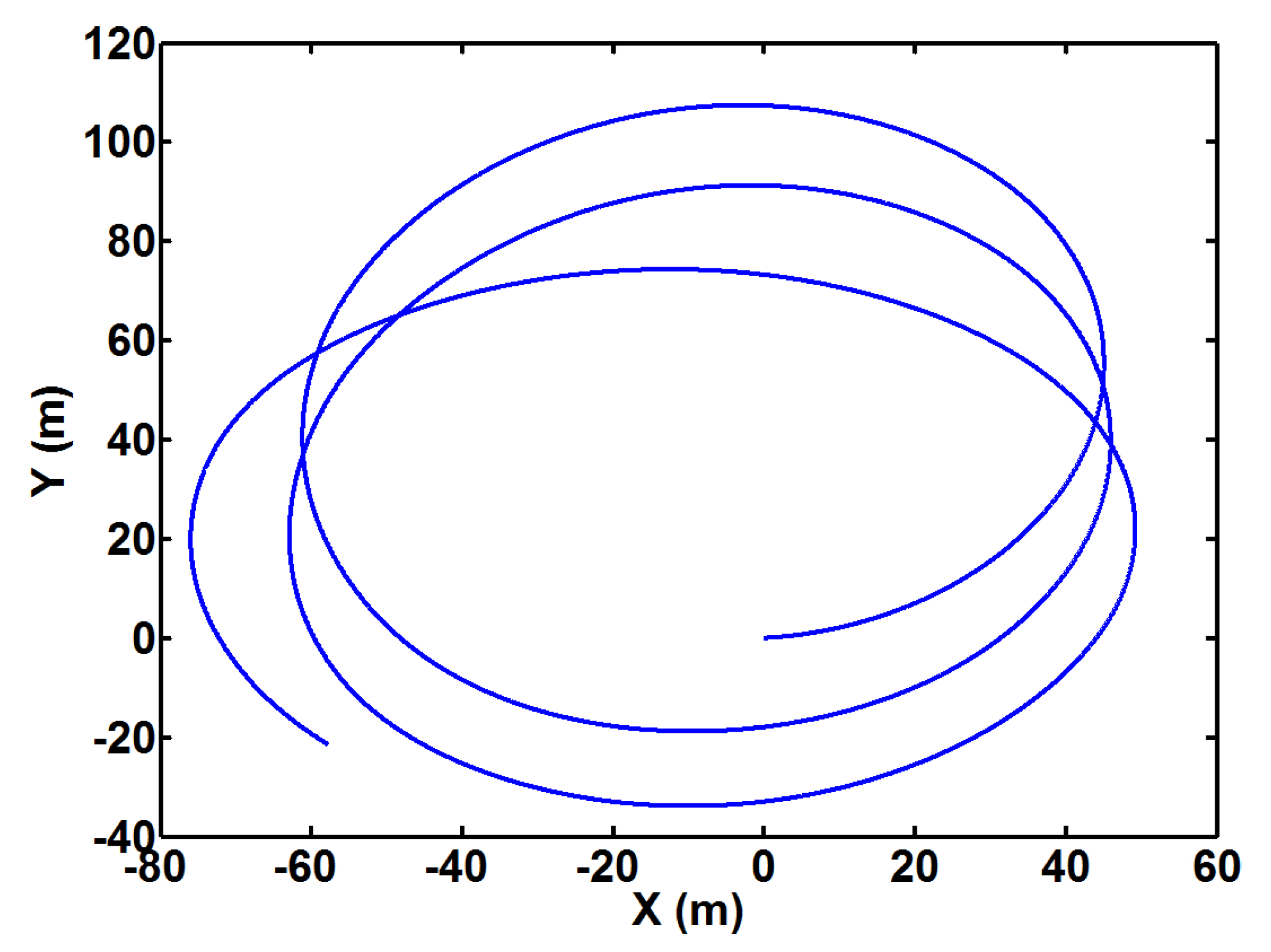
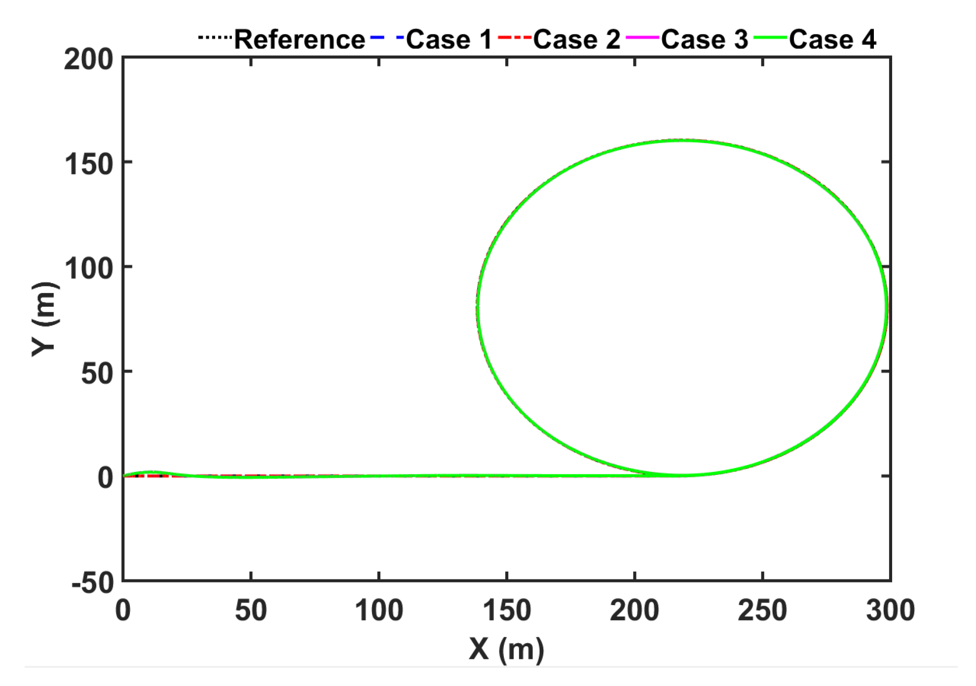
Now, the stability result of control law is as follows. The candidate Lyapunov function is constructed as

$$\begin{array}{c}\hfill V=\frac{1}{2}(S^2+\frac{1}{\gamma }{\tilde{\varphi }}^2).\end{array}$$

(18)

According to (13) and (16), the time derivative $\dot{V}$ is

$$\begin{array}{lll}\dot{V}& =& S\dot{S}+\frac{1}{\gamma }\tilde{\varphi }\dot{\widehat{\varphi }}\\ & =& S\left(F+B\mathbf{u}+D-{\ddot{P}}_d+\lambda \left(\dot{P}-{\dot{P}}_d\right)+\sigma \left(P-P_d\right)\right)\\ & & +\frac{1}{\gamma }\tilde{\varphi }\dot{\widehat{\varphi }}\\ & \le & S\left(F+B\mathbf{u}+\epsilon -{\ddot{P}}_d+\lambda \left(\dot{P}-{\dot{P}}_d\right)+\sigma \left(P-P_d\right)\right)\\ & & +\frac{1}{2}{S}^2\varphi h^{T}h+\frac{1}{2}+\frac{1}{\gamma }\tilde{\varphi }\dot{\widehat{\varphi }}\\ & \le & S\left(\frac{1}{2}S\varphi h^{T}h+F+B\mathbf{u}+\epsilon -{\ddot{P}}_d+\lambda \left(\dot{P}-{\dot{P}}_d\right)\right)\\ & & +S\sigma \left(P-P_d\right)+\tilde{\varphi }\left(\frac{1}{2}{S}^2{h}^{T}h-\kappa \widehat{\varphi }\right)+\frac{1}{2}.\end{array}$$

(19)

Substituting the control law (17) into (19), which can be rewritten as

$$\begin{array}{lll}\dot{V}& \le & -\mu S^2+\epsilon S-\eta \left|S\right|-\kappa \tilde{\varphi }\widehat{\varphi }+\frac{1}{2}\\ & \le & -\mu S^2-\kappa \tilde{\varphi }\widehat{\varphi }+\frac{1}{2}.\end{array}$$

(20)

Because ${(\tilde{\varphi }+\varphi )}^2\ge 0$, then ${\tilde{\varphi }}^2+2\tilde{\varphi }(\widehat{\varphi }-\tilde{\varphi })+{\varphi }^2\ge 0$, i.e., $2\tilde{\varphi }\widehat{\varphi }\ge {\tilde{\varphi }}^2-{\varphi }^2$, so the (21) is

$$\begin{array}{c}\hfill \dot{V}\le -\mu S^2-\frac{1}{2}\kappa {\tilde{\varphi }}^2+\frac{1}{2}\kappa {\varphi }^2+\frac{1}{2}.\end{array}$$

(21)

Define $q_1=\mu$, $q_2=\frac{1}{2}\kappa$, $\nabla =\frac{1}{2}\kappa {\varphi }^2+\frac{1}{2}$, then (21) becomes

$$\begin{array}{c}\hfill \dot{V}\le -q_1{S}^2-q_2{\tilde{\varphi }}^2+\nabla .\end{array}$$

(22)

Define $q=min\left\{q_1,q_2\right\}$, (22) can be rewritten as

$$\begin{array}{c}\hfill \dot{V}\le -2qV+\nabla .\end{array}$$

(23)

The (24) can be obtained by solving inequality (23).

$$\begin{array}{c}\hfill V\le \frac{\nabla }{2q}+\left(V\left(0\right)-\frac{\nabla }{2q}\right)e^{-2qt},\forall t>0.\end{array}$$

(24)

It can be seen from inequality (24) that V can eventually converge to a small set with boundary $\frac{\nabla }{2q}$. By choosing appropriate control parameters, the boundary can be made arbitrarily small. Therefore, it can be concluded that the system is uniformly ultimately bounded (UUB) stable.

5. Simulation Study

In this section, the effectiveness of the proposed control strategy is verified in four cases, including Case 1 (no delay response and no external disturbances), Case 2 (delay response without external disturbances), Case 3 (delay response and external disturbances without NNMLP) and Case 4 (delay response and external disturbances with NNMLP). The reference trajectory is generated by the identified model of USV, which was obtained in Section 2. The reference control variables are

$$n_d=2500r/\min ,{\delta }_d=\left\{\begin{array}{c}{0}^{\circ },t\le 50\mathrm{s}\hfill \\ 5^{\circ },t>50\mathrm{s}\hfill \end{array}\right..$$

In all four cases, the model uncertainties ${\mathsf{\Delta }}_u=0.2f_u$, ${\mathsf{\Delta }}_v=0.2f_v$, ${\mathsf{\Delta }}_r=0.2f_r$ will be added at 100 s. According to [37,38], the external disturbances are set to $b_u=1000\left[1+0.5sin\left(0.2t\right)+0.3cos\left(0.5t\right)\right]$, $b_v=1000[1+$$0.5sin\left(0.2t\right)+0.3cos\left(0.4t\right)]$, $b_r=1000\left[1+0.2sin\left(0.1t\right)+0.2cos\left(0.2t\right)\right]$. To show the influence of disturbances for the system more intuitively, the disturbance model is added to the simulation of turning test ($n=2500r/\min ,\delta =5^{\circ }$), and the output results are shown in Figure 7.

The control point P is chosen at the bow position with $l=L/2$. The initial state of vessel is $\left(x,y,\psi ,u,v,r\right)\left(0\right)=0$. The control parameters are $\lambda =diag[0.3,0.3]$, $\sigma =diag[0.05,0.05]$, $\mu =diag[15,15]$, $\eta =diag[0.3,0.3]$, $\gamma =diag[10,10]$, and $\kappa =diag[0.0005,0.0005]$.

With the designed controller, the vessel tracks the reference trajectory. The results of tracking trajectory are shown in Figure 8. It can be seen from the results that with system uncertainties and external disturbances, the vessel can follow the reference trajectory well. The tracking errors are drawn in Figure 9. For Cases 3 and 4, although Case 3 can also control the trajectory tracking under disturbance, NNMPL technology accelerates the convergence speed of the controller. At the same time, the tracking errors of Case 3 are higher than that of Case 4. In addition, as the steady-state behavior from 130 s to 200 s clearly shows in Figure 9, the tracking errors of Case 3 are less than 0.10 m, i.e., $\left|X_e\right|\le 0.10$ m, $\left|Y_e\right|\le 0.10$ m, while in Case 4 they are less than 0.07 m. It can be seen that NNMLP enhances the tracking accuracy of the controller. Therefore, the tracking errors of the proposed scheme can be converged well near the zero point in Case 4.

The thruster speed n and propulsion angle $\delta$ as control inputs are described in Figure 10. It can be seen that when the system uncertainty is added at 100 s, the thruster speed n deviates from the reference value. In four cases, the results of control inputs are different. In Case 1, the control inputs can quickly keep up with the reference value without oscillation. The oscillation in Case 2 is due to the effect of the actuator delay. In Cases 3 and 4, the control input deviates completely from the reference value because the actuators need to generate extra forces to accommodate the uncertainties and external disturbance.

6. Conclusions

A trajectory tracking control framework is proposed for vector propulsion USV with external disturbances and system uncertainties. In this paper, the mathematical model of vector propulsion USV is established by analyze the actuator distribution and its model parameters are identified through field experiments. Because the model is an incomplete underactuated system, the virtual control point method is used to design the controller to solve the unstable internal dynamics caused by the strong coupling between the sway force and yaw moment, which provides a way for the future research on the motion control of vector propulsion USV. Finally, an adaptive sliding mode trajectory tracking controller based on NNMLP theory is designed. The simulation results confirm that the designed controller cannot only control the incomplete underactuated USV system, but also stabilize the external disturbances and uncertainties. It should be pointed out that although the delay response of actuator was tested in the simulation experiment, and the results confirm that the current controller is also robust to the delay response, it will also cause the control input oscillation, which should be avoided as far as possible for the actuator. Therefore, in the future research, this issue should be taken into account in the design of the controller.

References

1. Liu, Z.; Zhang, Y.; Yu, X.; Yuan, C. Unmanned surface vehicles: An overview of developments and challenges. Annu. Rev. Control 2016, 41, 71–93. [Google Scholar] [CrossRef]
2. Qiao, D.L.; Liu, G.Z.; Zhang, J.; Zhang, Q.Y.; Wu, G.X.; Dong, F. (MC)-C-3: Multimodel-and-Multicue-Based Tracking by Detection of Surrounding Vessels in Maritime Environment for USV. Electronics 2019, 8, 723. [Google Scholar] [CrossRef] [Green Version]
3. Zhang, G.; Zhang, X. A novel DVS guidance principle and robust adaptive path-following control for underactuated ships using low frequency gain-learning. ISA Trans. 2015, 56, 75–85. [Google Scholar] [CrossRef]
4. Yao, W.; Zhang, J.; Liu, Y.; Zhou, M.; Sun, M.; Zhang, G. Improved Vector Control for Marine Podded Propulsion Control System Based on Wavelet Analysis. J. Coast. Res. 2015, 73, 54–59. [Google Scholar] [CrossRef]
5. Gierusz, W. Modelling the Dynamics of Ships with Different Propulsion Systems for Control Purpose. Polish Marit. Res. 2016, 23, 31–36. [Google Scholar] [CrossRef]
6. Abkowitz, M.A. Lectures on Ship Hydrodynamics—Steering and Maneuverability; Technical Report; Hydro’ and Aerodynamic’s Laboratory: Lyngby, Denmark, 1964. [Google Scholar]
7. Norrbin, N.H. Theory and observation on the use of a mathematical model for ship maneuvering in deep and confined waters. In Proceedings of the 8th Symposium on Naval Hydrodynamics, Pasadena, CA, USA, 24–28 August 1970. [Google Scholar]
8. Ogawa, A.; Koyama, T.; Kijima, K. MMG report-I, on the mathematical model of ship manoeuvring. Bull. Soc. Naval Archit. Jpn. 1977, 575, 22–28. [Google Scholar]
9. Yasukawa, H.; Yoshimura, Y. Introduction of MMG standard method for ship maneuvering predictions. J. Mar. Sci. Technol. 2015, 20, 37–52. [Google Scholar] [CrossRef] [Green Version]
10. Lu, X.j.; Zhou, Q.d.; Fang, B. Hydrodynamic performance of distributed pump-jet propulsion system for underwater vehicle. J. Hydrodyn. 2014, 26, 523–530. [Google Scholar] [CrossRef]
11. Xiong, Y.; Zhang, K.; Wang, Z.Z.; Qi, W.J. Numerical and Experimental Studies on the Effect of Axial Spacing on Hydrodynamic Performance of the Hybrid CRP Pod Propulsion System. China Ocean Eng. 2016, 30, 627–636. [Google Scholar] [CrossRef]
12. Wang, Z.Z.; Xiong, Y.; Wang, R.; Zhong, C.h. Numerical investigation of the scale effect of hydrodynamic performance of the hybrid CRP pod propulsion system. Appl. Ocean Res. 2016, 54, 26–38. [Google Scholar] [CrossRef]
13. Gierusz, W. Simulation model of the LNG carrier with podded propulsion Part I: Forces generated by pods. Ocean Eng. 2015, 108, 105–114. [Google Scholar] [CrossRef]
14. Gierusz, W. Simulation model of the LNG carrier with podded propulsion, Part II: Full model and experimental results. Ocean Eng. 2016, 123, 28–44. [Google Scholar] [CrossRef]
15. Reichel, M. Prediction of manoeuvring abilities of 10000 DWT pod-driven coastal tanker. Ocean Eng. 2017, 136, 201–208. [Google Scholar] [CrossRef]
16. Mu, D.D.; Wang, G.F.; Fan, Y.S. Design of Adaptive Neural Tracking Controller for Pod Propulsion Unmanned Vessel Subject to Unknown Dynamics. J. Electr. Eng. Technol. 2017, 12, 2365–2377. [Google Scholar]
17. Su, Y.X.; Zheng, C.H.; Mercorelli, P. Nonlinear PD Fault-Tolerant Control for Dynamic Positioning of Ships With Actuator Constraints. IEEE/ASME Trans. Mechatron. 2017, 22, 1132–1142. [Google Scholar] [CrossRef]
18. Xie, W.; Ma, B.; Huang, W.; Zhao, Y. Global trajectory tracking control of underactuated surface vessels with non-diagonal inertial and damping matrices. Nonlinear Dyn. 2018, 92, 1481–1492. [Google Scholar] [CrossRef]
19. Abdelaal, M.; Fraenzle, M.; Hahn, A. Nonlinear Model Predictive Control for trajectory tracking and collision avoidance of underactuated vessels with disturbances. Ocean Eng. 2018, 160, 168–180. [Google Scholar] [CrossRef]
20. Jin, J.C.; Zhang, J.; Liu, D.Q. Design and Verification of Heading and Velocity Coupled Nonlinear Controller for Unmanned Surface Vehicle. Sensors 2018, 18, 3427. [Google Scholar] [CrossRef] [Green Version]
21. Consolini, L.; Tosques, M. A Minimum Phase Output in the Exact Tracking Problem for the Nonminimum Phase Underactuated Surface Ship. IEEE Trans. Autom. Control 2012, 57, 3174–3180. [Google Scholar] [CrossRef]
22. Toussaint, G.J.; Basar, T.; Bullo, F. Tracking for nonlinear underactuated surface vessels with generalized forces. In Proceedings of the 2000 IEEE International Conference on Control Applications, Anchorage, AK, USA, 27 September 2000; pp. 355–360. [Google Scholar]
23. Toussaint, G.J.; Basar, T.; Bullo, F. H-infinity-Optimal Tracking Control Techniques for Nonlinear Underactuated Systems. In Proceedings of the 41st IEEE Conference on Decision and Control, Las Vegas, NV, USA, 10–13 December 2002; pp. 2078–2083. [Google Scholar]
24. Sun, X.J.; Wang, G.F.; Fan, Y.S.; Mu, D.D.; Qiu, B.B. Collision Avoidance Using Finite Control Set Model Predictive Control for Unmanned Surface Vehicle. Appl. Sci. 2018, 8, 926. [Google Scholar] [CrossRef] [Green Version]
25. Sun, X.J.; Wang, G.F.; Fan, Y.S.; Mu, D.D.; Qiu, B.B. An Automatic Navigation System for Unmanned Surface Vehicles in Realistic Sea Environments. Appl. Sci. 2018, 8, 193. [Google Scholar]
26. Dong, W.; Guo, Y. Global time-varying stabilization of underactuated surface vessel. IEEE Trans. Autom. Control 2005, 50, 859–864. [Google Scholar] [CrossRef]
27. Fossen, T.I. Handbook of Marine Craft Hydrodynamics and Motion Control; John Wiley & Sons: Hoboken, NJ, USA, 2011. [Google Scholar]
28. Zhang, G.Q.; Deng, Y.J.; Zhang, W.D.; Huang, C.F. Novel DVS guidance and path-following control for underactuated ships in presence of multiple static and moving obstacles. Ocean Eng. 2018, 170, 100–110. [Google Scholar] [CrossRef]
29. Liu, Y.; You, J.; Ding, F. Iterative identification for multiple-input systems based on auxiliary model-orthogonal matching pursuit. Control Decis. 2019, 34, 787–792. [Google Scholar]
30. Ding, F. System Identification: Performance Analysis of Identification Methods; Science Press: Beijing, China, 2014. [Google Scholar]
31. Sun, X.; Wang, G.; Fan, Y.; Mu, D.; Qiu, B. A Formation Collision Avoidance System for Unmanned Surface Vehicles With Leader-Follower Structure. IEEE Access 2019, 7, 24691–24702. [Google Scholar] [CrossRef]
32. Jia, X.l.; Yang, Y.s. The Mathematical Model of Ship Motion Mechanism Modeling and Identification Modeling; Dalian Maritime University Press: Dalian, China, 1999. [Google Scholar]
33. Morel, Y.; Leonessa, A. Indirect adaptive control of a class of marine vehicles. Int. J. Adapt. Control Signal Process. 2010, 24, 261–274. [Google Scholar] [CrossRef] [Green Version]
34. Bu, X.W.; Wu, X.Y.; Wei, D.Z.; Huang, J.Q. Neural-approximation-based robust adaptive control of flexible air-breathing hypersonic vehicles with parametric uncertainties and control input constraints. Inf. Sci. 2016, 346, 29–43. [Google Scholar] [CrossRef]
35. Bu, X.W.; Wu, X.Y.; Huang, J.Q.; Ma, Z.; Zhang, R. Minimal-learning-parameter based simplified adaptive neural back-stepping control of flexible air-breathing hypersonic vehicles without virtual controllers. Neurocomputing 2016, 175, 816–825. [Google Scholar] [CrossRef]
36. Elmokadem, T.; Zribi, M.; Youcef-Toumi, K. Trajectory tracking sliding mode control of underactuated AUVs. Nonlinear Dyn. 2016, 84, 1079–1091. [Google Scholar] [CrossRef] [Green Version]
37. Pan, C.Z.; Lai, X.Z.; Yang, S.X.; Wu, M. A biologically inspired approach to tracking control of underactuated surface vessels subject to unknown dynamics. Expert Syst. Appl. 2015, 42, 2153–2161. [Google Scholar] [CrossRef]
38. Hu, X.; Du, J.L.; Sun, Y.Q. Robust Adaptive Control for Dynamic Positioning of Ships. IEEE J. Ocean. Eng. 2017, 42, 826–835. [Google Scholar] [CrossRef]
Figure 1. The Lanxin USV.
Electronics 09 00022 g001
Figure 2. The power propulsion system of USV.
Electronics 09 00022 g002
Figure 3. The description of vector propulsion USV motion variables.
Electronics 09 00022 g003
Figure 4. The comparison results of two tests. (a) 10 / 10 zig-zag test; (b) 10 turning test.
Electronics 09 00022 g004
Figure 5. The comparison results about the state quantities of vessel. (a) 10 / 10 zig-zag test; (b) 10 turning test.
Electronics 09 00022 g005
Figure 6. The virtual control point P.
Electronics 09 00022 g006
Figure 7. The simulation of turning test with disturbances.
Electronics 09 00022 g007
Figure 8. The trajectory tracking results with four Cases.
Electronics 09 00022 g008
Figure 9. The trajectory tracking errors X e and Y e with four Cases.
Electronics 09 00022 g009
Figure 10. The trajectory tracking control inputs.
Electronics 09 00022 g010