Grid Reconfiguration Method for Off-Grid DOA Estimation


Abstract
1. Introduction
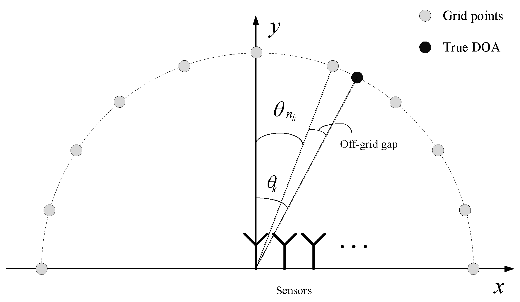
2. Data Model
3. The GRDOA Algorithm
3.1. Sparse Bayesian Formulation
3.2. Grid Update
3.3. Grid Fission
3.4. Criteria of GRDOA
3.4.1. Grid Selection Criterion in the Initial Estimation
3.4.2. The Stop Criterion of the Initial Estimation
3.4.3. The Stop Criterion of the Fine Estimation
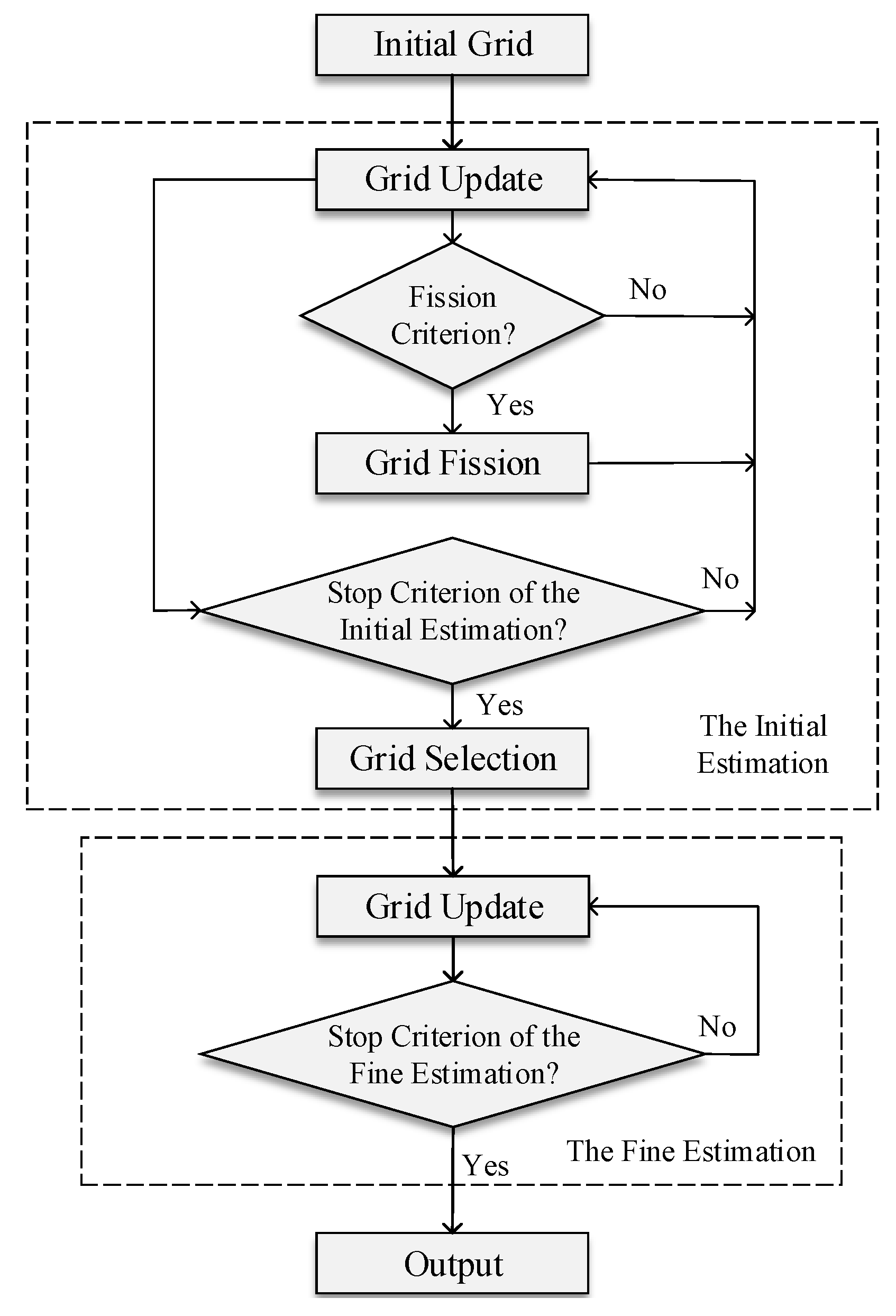
3.5. Operating Instruction of GRDOA
4. Simulation
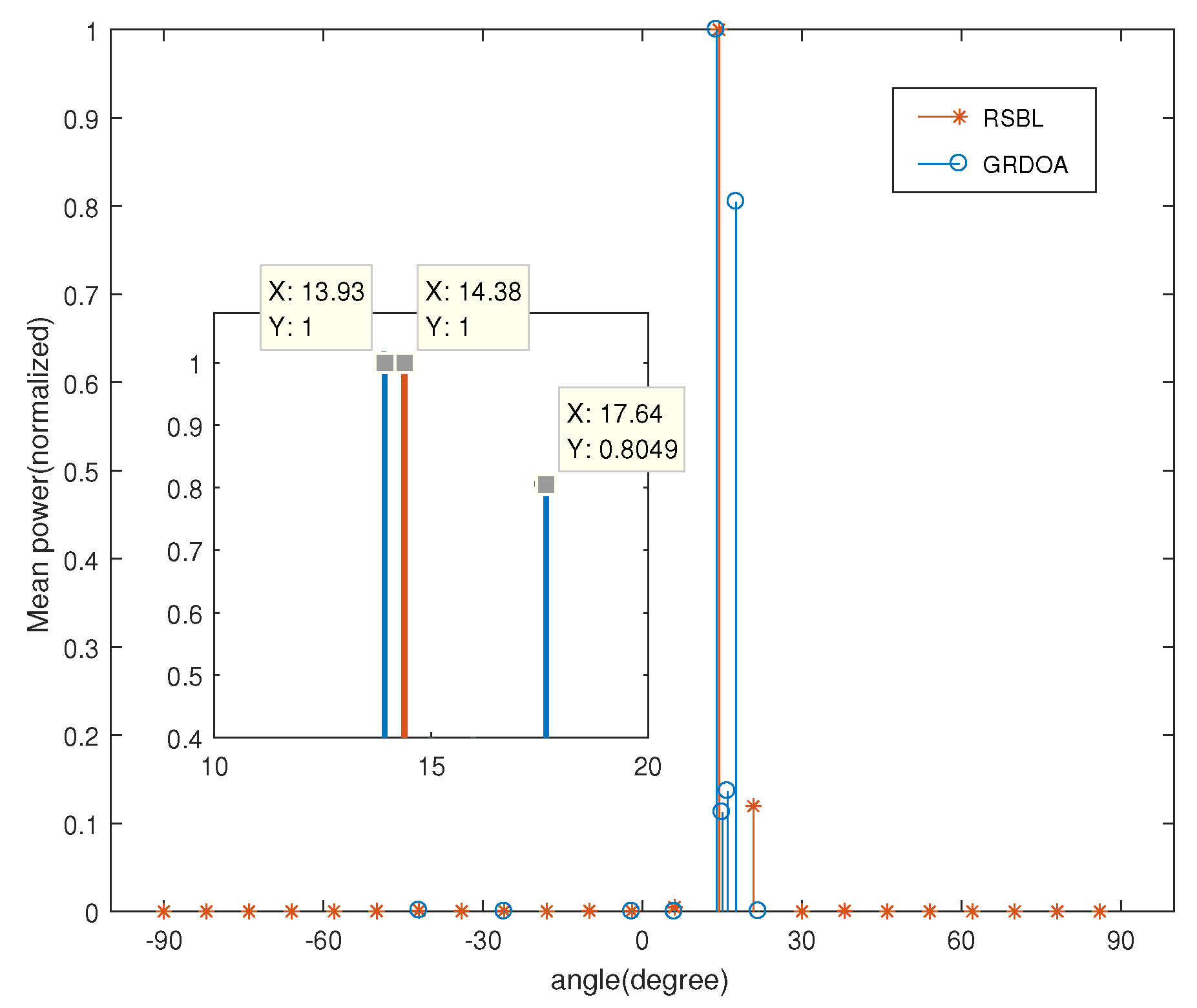
4.1. Spatial Spectrum
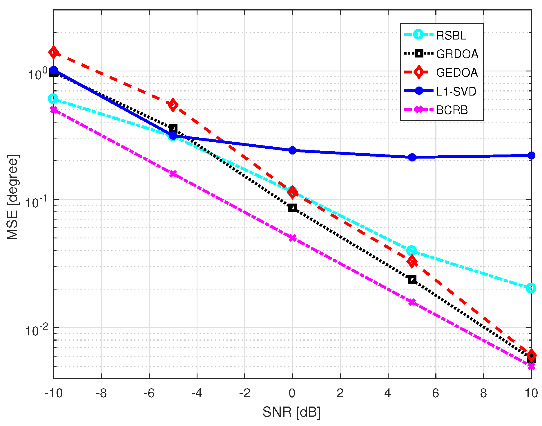
4.2. Performance Analysis
4.3. Compared with GEDOA
5. Conclusions
Author Contributions
Funding
Acknowledgments
Conflicts of Interest
References
- Liu, L.; Zhang, X.; Chen, P. Compressed sensing-based DOA estimation with antenna phase errors. Electronics 2019, 8, 294. [Google Scholar] [CrossRef]
- Li, S.; Wu, H.; Jin, L. Codebook-Aided DOA Estimation Algorithms for Massive MIMO System. Electronics 2019, 8, 26. [Google Scholar] [CrossRef]
- Wang, X.; Huang, M.; Shen, C.; Meng, D. Robust vehicle localization exploiting two based stations cooperation: A MIMO radar perspective. IEEE Access 2018, 6, 48747–48755. [Google Scholar] [CrossRef]
- Wang, H.; Wan, L.; Dong, M.; Ota, K.; Wang, X. Assistant vehicle localization based on three collaborative base stations via SBL-based robust DOA estimation. IEEE Internet Things J. 2019, 6, 5766–5777. [Google Scholar] [CrossRef]
- Wan, L.; Han, G.; Shu, L.; Chan, S.; Zhu, T. The application of DOA estimation approach in patient tracking systems with high patient density. IEEE Trans. Ind. Inform. 2016, 12, 2353–2364. [Google Scholar] [CrossRef]
- Schmidt, R. Multiple emitter location and signal parameter estimation. IEEE Trans. Antennas Propag. 1986, 34, 276–280. [Google Scholar] [CrossRef]
- Roy, R.; Kailath, T. ESPRIT-estimation of signal parameters via rotational invariance techniques. IEEE Trans. Acoust. Speech Signal Process. 1989, 37, 984–995. [Google Scholar] [CrossRef]
- Donoho, D.L. Compressed sensing. IEEE Trans. Inf. Theory 2006, 52, 1289–1306. [Google Scholar] [CrossRef]
- Pinchera, D.; Migliore, M.D.; Lucido, M.; Schettino, F.; Panariello, G. Efficient Large Sparse Arrays Synthesis by Means of Smooth Re-Weighted L1 Minimization. Electronics 2019, 8, 83. [Google Scholar] [CrossRef]
- Gong, P.; Wang, W.Q.; Li, F.; So, H.C. Sparsity-aware transmit beamspace design for FDA-MIMO radar. Signal Process. 2018, 144, 99–103. [Google Scholar] [CrossRef]
- Pinchera, D.; Migliore, M.D.; Lucido, M.; Schettino, F.; Panariello, G. A compressive-sensing inspired alternate projection algorithm for sparse array synthesis. Electronics 2017, 6, 3. [Google Scholar] [CrossRef]
- Pinchera, D.; Migliore, M.D. Comparison guidelines and benchmark procedure for sparse array synthesis. Prog. Electromagn. Res. M 2016, 52, 129–139. [Google Scholar] [CrossRef]
- Bucci, O.M.; Perna, S.; Pinchera, D. Synthesis of isophoric sparse arrays allowing zoomable beams and arbitrary coverage in satellite communications. IEEE Trans. Antennas Propag. 2015, 63, 1445–1457. [Google Scholar] [CrossRef]
- Migliore, M.D. On the sampling of the electromagnetic field radiated by sparse sources. IEEE Trans. Antennas Propag. 2015, 63, 553–564. [Google Scholar] [CrossRef]
- Migliore, M.D. A simple introduction to compressed sensing/sparse recovery with applications in antenna measurements. IEEE Antennas Propag. Mag. 2014, 2, 14–26. [Google Scholar] [CrossRef]
- Pinchera, D.; Migliore, M.D. Effective sparse array synthesis using a generalized alternate projection algorithm. In Proceedings of the IEEE Conference on Antenna Measurements & Applications (CAMA), Antibes Juan-les-Pins, France, 16–19 November 2014; pp. 1–2. [Google Scholar]
- Bucci, O.M.; Isernia, T.; Perna, S.; Pinchera, D. Isophoric sparse arrays ensuring global coverage in satellite communications. IEEE Trans. Antennas Propag. 2014, 62, 1607–1618. [Google Scholar] [CrossRef]
- Costanzo, S.; Borgia, A.; Di Massa, G.; Pinchera, D.; Migliore, M.D. Radar array diagnosis from undersampled data using a compressed sensing/sparse recovery technique. J. Electr. Comput. Eng. 2013, 2013, 8. [Google Scholar] [CrossRef]
- Migliore, M.D.; Pinchera, D. Compressed sensing in electromagnetics: Theory, applications and perspectives. In Proceedings of the 5th European Conference on Antennas and Propagation (EUCAP), Rome, Italy, 11–15 April 2011. [Google Scholar]
- Shi, Z.; Zhou, C.; Gu, Y.; Goodman, N.A.; Qu, F. Source estimation using coprime array: A sparse reconstruction perspective. IEEE Sens. J. 2016, 17, 755–765. [Google Scholar] [CrossRef]
- Gong, P.; Wang, W.Q.; Wan, X. Adaptive weight matrix design and parameter estimation via sparse modeling for MIMO radar. Signal Process. 2017, 139, 1–11. [Google Scholar] [CrossRef]
- Zhou, C.; Gu, Y.; Fan, X.; Shi, Z.; Mao, G.; Zhang, Y.D. Direction-of-arrival estimation for coprime array via virtual array interpolation. IEEE Trans. Signal Process. 2018, 66, 5956–5971. [Google Scholar] [CrossRef]
- Chen, P.; Cao, Z.; Chen, Z.; Liu, L.; Feng, M. Compressed sensing-based DOA estimation with unknown mutual coupling effect. Electronics 2018, 7, 424. [Google Scholar] [CrossRef]
- Chen, P.; Cao, Z.; Chen, Z.; Wang, X. Off-Grid DOA Estimation Using Sparse Bayesian Learning in MIMO Radar with Unknown Mutual Coupling. IEEE Trans. Signal Process. 2019, 67, 208–220. [Google Scholar] [CrossRef]
- Duan, H. MSM-FOCUSS for distributed compressive sensing and wideband DOA estimation. In Proceedings of the 2014 19th International Conference on Digital Signal Processing, Hong Kong, China, 20–23 August 2014; pp. 400–403. [Google Scholar]
- Malioutov, D.; Cetin, M.; Willsky, A. A sparse signal reconstruction perspective for source localization with sensor arrays. IEEE Trans. Signal Process. 2005, 53, 3010–3022. [Google Scholar] [CrossRef]
- Stoica, P.; Babu, P.; Jian, L. SPICE: A sparse covariance-based estimation method for array processing. IEEE Trans. Signal Process. 2011, 59, 629–638. [Google Scholar] [CrossRef]
- Wipf, D.P.; Rao, B.D. An empirical Bayesian strategy for solving the simultaneous sparse approximation problem. IEEE Trans. Signal Process. 2007, 55, 3704–3716. [Google Scholar] [CrossRef]
- Zhu, H.; Leus, G.; Giannakis, G. Sparsity-cognizant total least-squares for perturbed compressive sampling. IEEE Trans. Signal Process. 2011, 59, 2002–2016. [Google Scholar] [CrossRef]
- Yang, Z.; Xie, L.; Zhang, C. Off-grid direction of arrival estimation using sparse Bayesian inference. IEEE Trans. Signal Process. 2013, 61, 38–43. [Google Scholar] [CrossRef]
- Wu, X.; Zhu, W.P.; Yan, J. Direction of arrival estimation for off-grid signals based on sparse Bayesian learning. IEEE Sens. J. 2016, 16, 2004–2016. [Google Scholar] [CrossRef]
- Dai, J.; Bao, X.; Xu, W.; Chang, C. Root sparse Bayesian learning for off-grid DOA estimation. IEEE Signal Process. Lett. 2017, 24, 46–50. [Google Scholar] [CrossRef]
- Wang, Q.; Zhao, Z.; Chen, Z.; Nie, Z. Grid evolution method for DOA estimation. IEEE Trans. Signal Process. 2018, 66, 2374–2383. [Google Scholar] [CrossRef]
- Yang, Z.; Xie, L. On gridless sparse methods for multi-snapshot DOA estimation. In Proceedings of the 2016 IEEE International Conference on Acoustics, Speech and Signal Processing (ICASSP), Shanghai, China, 20–25 March 2016; pp. 3236–3240. [Google Scholar]
- Wu, X.; Zhu, W.P.; Yan, J. A fast gridless covariance matrix reconstruction method for one-and two-dimensional direction-of-arrival estimation. IEEE Sens. J. 2017, 17, 4916–4927. [Google Scholar] [CrossRef]
- Wu, X.; Zhu, W.P.; Yan, J.; Zhang, Z. A Spatial Filtering Based Gridless DOA Estimation Method for Coherent Sources. IEEE Access 2018, 6, 56402–56410. [Google Scholar] [CrossRef]
- Zhang, X.; Liu, L.; Chen, P.; Cao, Z.; Chen, Z. Gridless Sparse Direction Finding Method for Correlated Signals with Gain-Phase Errors. Electronics 2019, 8, 557. [Google Scholar] [CrossRef]
- Wang, H.; Wang, X.; Wan, L.; Huang, M. Robust Sparse Bayesian Learning for Off-Grid DOA Estimation with Non-Uniform Noise. IEEE Access 2018, 6, 64688–64697. [Google Scholar] [CrossRef]
- Shutin, D.; Fleury, B.H. Sparse variational Bayesian SAGE algorithm with application to the estimation of multipath wireless channels. IEEE Trans. Signal Process. 2011, 59, 3609–3623. [Google Scholar] [CrossRef]
- Ji, S.; Xue, Y.; Carin, L. Bayesian compressive sensing. IEEE Trans. Signal Process. 2008, 56, 2346–2356. [Google Scholar] [CrossRef]
- Dempster, A.P. Maximum likelihood from incomplete data via the EM algorithm. J. R. Stat. Soc. 1977, 39, 1–38. [Google Scholar] [CrossRef]


| The Proposed GRDOA Algorithm |
|---|
| (1) Input: and ; |
| (2) Conduct the initial estimation: |
| (a) Initialize: and , D is set as a half of the grid interval. |
| (b) Conduct the grid update process as follows: |
| Compute the posterior moments and using Equations (10) and (11). |
| Update and using Equations (12) and (13), refine using (17). |
| (c) If , conduct the grid fission process: |
| Generate new grid point using Equation (18) or Equation (19). |
| Update and according to Equation (21) and (23). |
| (d) Iterate (b)–(c) until reaching the stop criterion of the initial estimation. |
| (e) Form a new grid according to the grid selection criterion. |
| (3) Conduct the fine estimation |
| (a) Input according to the reconfigured grid . |
| (b) Initialize and . |
| (c) Conduct the grid update process (presented above) until reaching the stop |
| criterion of the fine estimation. |
| (4) Output: and the final grid; |
| (5) Achieve off-grid DOA estimation through 1D spectrum search on the final grid. |
| IGI [] | 2 | 4 | 6 | 8 | 10 |
|---|---|---|---|---|---|
| CPU time of RSBL [s] | 13 | 7.18 | 6.19 | 5.15 | 4.38 |
| CPU time of GRDOA [s] | 4.72 | 4.49 | 3.22 | 3.37 | 3.67 |
| CPU time of GEDOA [s] | 5.19 (IGI = ) | ||||
| CPU time of -SVD [s] | 24.9 (IGI = ) | ||||
© 2019 by the authors. Licensee MDPI, Basel, Switzerland. This article is an open access article distributed under the terms and conditions of the Creative Commons Attribution (CC BY) license (http://creativecommons.org/licenses/by/4.0/).
Share and Cite
Ling, Y.; Gao, H.; Ru, G.; Chen, H.; Li, B.; Cao, T. Grid Reconfiguration Method for Off-Grid DOA Estimation. Electronics 2019, 8, 1209. https://doi.org/10.3390/electronics8111209
Ling Y, Gao H, Ru G, Chen H, Li B, Cao T. Grid Reconfiguration Method for Off-Grid DOA Estimation. Electronics. 2019; 8(11):1209. https://doi.org/10.3390/electronics8111209
Chicago/Turabian StyleLing, Yun, Huotao Gao, Guobao Ru, Haitao Chen, Boya Li, and Ting Cao. 2019. "Grid Reconfiguration Method for Off-Grid DOA Estimation" Electronics 8, no. 11: 1209. https://doi.org/10.3390/electronics8111209
APA StyleLing, Y., Gao, H., Ru, G., Chen, H., Li, B., & Cao, T. (2019). Grid Reconfiguration Method for Off-Grid DOA Estimation. Electronics, 8(11), 1209. https://doi.org/10.3390/electronics8111209