EEG-Based 3D Visual Fatigue Evaluation Using CNN

Abstract

Visual fatigue evaluation plays an important role in applications such as virtual reality since the visual fatigue symptoms always affect the user experience seriously. Existing visual evaluation methods require hand-crafted features for classification, and conduct feature extraction and classification in a separated manner. In this paper, we conduct a designed experiment to collect electroencephalogram (EEG) signals of various visual fatigue levels, and present a multi-scale convolutional neural network (CNN) architecture named MorletInceptionNet to detect visual fatigue using EEG as input, which exploits the spatial-temporal structure of multichannel EEG signals. Our MorletInceptionNet adopts a joint space-time-frequency features extraction scheme in which Morlet wavelet-like kernels are used for time-frequency raw feature extraction and inception architecture are further used to extract multi-scale temporal features. Then, the multi-scale temporal features are concatenated and fed to the fully connected layer for visual fatigue evaluation using classification. In experiment evaluation, we compare our method with five state-of-the-art methods, and the results demonstrate that our model achieve overally the best performance better performance for two widely used evaluation metrics, i.e., classification accuracy and kappa value. Furthermore, we use input-perturbation network-prediction correlation maps to conduct in-depth analysis into the reason why the proposed method outperforms other methods. The results suggest that our model is sensitive to the perturbation of $\beta$ (14–30 Hz) and $\gamma$ (30–40 Hz) bands. Furthermore, their spatial patterns are of high correlation with that of the corresponding power spectral densities which are used as evaluation features traditionally. This finding provides evidence of the hypothesis that the proposed model can learn the joint time-frequency-space features to distinguish fatigue levels automatically.

1. Introduction

Compared with 2D content, 3D content can provide users with highly realistic sensations and a sense of presence, which can improve their experience significantly. However, periods of extended viewing 3D content often cause symptoms such as headache and nausea, thus causing negative effects on user experience. These undesirable effects, which have been labeled the 3D visual fatigue, seriously hinder the development of 3D industry [1]. Therefore, the evaluation of 3D visual fatigue has received considerable attention.

Vast studies have been conducted to explore reasonable indicators for visual fatigue evaluation using optometric devices on visual system [2,3,4]. However, in most cases these measurements are generally costly, time-consuming, and are usually conducted with only small numbers of participants, making the results less reliable [1]. Subsequently, features extracted from physiological signals such as electrooculogram (EOG) and electrocardiogram (ECG) are adopted for evaluating visual fatigue [5,6]. Although these features are found to be statistically associated with visual fatigue, they are still not ideally indicators. Since mental fatigue is supposed as one aspect of 3D visual fatigue, these features can hardly represent psychological changes [7].

Recently, researches have opened up the possibility for visual fatigue assessment with noninvasive approaches based on electroencephalography (EEG) [1]. EEG signals record integration of spontaneous electrical activities of a large number of brain cells from the scalp, which is closely related with mental and physical states [8]. All event-related potentials in EEG are limited in duration and in frequency. The majority of events activate distinct brain regions [9]. This means researchers can extract features from space, time, and frequency dimensions of the EEG data to build efficient classification models for visual fatigue evaluation. Traditionally, the most popular features for visual fatigue evaluation are time-frequency features (e.g., power spectral), which can be obtained by time-frequency transformation (e.g., wavelet transformation). Power spectral of various frequency bands are proven to be related with visual fatigue levels statistically, even their combinations can also be indicators of visual fatigue classification [10]. These extracted features are then passed as input of classifiers (e.g., support vector machine (SVM)) to perform the final decoding. However, these traditional methods have a main drawback that the performance of classification is heavily reliant upon the designed features extracted from original EEG signals. On the other hand, the performance of classification relies on the prior knowledge of experts who design these features and the process of manually selected usefully features is always time-consuming. Moreover, even though the statistically significant features are obtained, traditional methods are still hard to achieve desirable results.

Recently, deep learning (DL) techniques have shown distinctive capabilities in detection [11], speech recognition [12], and time series classification [13]. Instead of separated feature extraction from classification, DL methods learn subject-specific features guided by classification tasks automatically and can be trained as an end-to-end measure [13,14,15,16,17]. This means feeding raw EEG signals into the network can obtain the predicted label corresponding to the input in the end. Although these approaches achieve competitive performances in EEG classification compared with traditional methods like FBCSP-SVM, there is still substantial room for in-depth research and improvement regarding accuracy, interpretability, and robustness. Previous methods only capture temporal and spatial information contained within EEG signals, however, the multi-scale frequency domain information, which is supposed as one of the most important features in EEG-based classification, is not extracted.

In this paper, we introduce deep learning techniques into EEG-based 3D fatigue assessment for the first time. We conduct a designed experiment to collect EEG signals being various fatigue levels and then apply the proposed MorletInceptionNet to perform automatic visual fatigue evaluation. Compared with state-of-the-art methods, characteristics of three scales are considered simultaneously in this paper by concatenating outputs of three inception modules in depth. The inception modules are of different kernel size and implement a joint space-time-frequency feature extracting with various time-scales. In addition, a $1\times 1$ convolutional layer is inserted to transform the sparse matrix into a relatively dense submatrix with the purpose of boosting performance. The proposed model is evaluated on our own visual fatigue evaluation dataset compared with other deep learning models. Our MorletInceptionNet has significant improvement over other deep learning methods.

The rest of this paper is organized as follows. Related work is introduced in Section 2. The motivations, network architecture, and configurations are described in Section 3. Systematic introduction of visual fatigue experiment and the acquisition and preprocessing of EEG signal are then introduced in Section 4. Then the evaluation of the proposed network and related analysis are described in Section 5. The conclusion and main findings are provided in Section 6.

2. Related Work

There are several studies managing to develop methods for 3D visual fatigue evaluation. Recently, many researchers started to use features extracted from EEG, such as power spectral density (PSD), in various frequency bands (delta ($\delta$) 1–3 Hz, theta ($\theta$) 4–7 Hz, alpha ($\alpha$) 8–13 Hz, beta ($\beta$) 14–30 Hz, and gamma ($\gamma$) 30–40 Hz). Vast literatures have investigated the statistical relationship between PSD of various frequency band and visual fatigue levels. Kim et al. found the PSD of $\beta$ and $\theta$ increased significantly when subjects viewing uncomfortable 3D pictures, while PSD of $\alpha$ decreased [18]. Yin et al. found the PSD in occipital and frontal areas increase significantly as 3D visual fatigue becomes severe [19]. Guo et al. induced 3D visual fatigue using random-dot stereograms (RDS) to investigate the relationship between PSD of EEG and visual fatigue, and they found a significant increase for PSD in $\alpha$ bands [20]. Hsu et al. points out that the power ratio of $\beta$ and $\alpha$ bands in EEG were the most effective power indexes for the visual fatigue evaluation [21]. Chen et al. characterize the EEG signals using the gravity frequency and the power spectral entropy, which served as indicators to evaluate the level of visual fatigue [10]. However, these methods only take advantage of temporal spectral information in EEG, ignoring the spatial information.

Inspired by the spatial property of EEG, researchers have proposed some classification methods based on the common spatial patterns (CSPs) algorithm [22]. The CSP algorithm finds a set of linear transformations (i.e., spatial filters) that maximize the distance of multiple classes (i.e., different visual fatigue levels). Then power spectrals of estimated filtered channels are calculated as the representation of the EEG and are fed into a linear classifier, such as SVM, leading to good performance. However, this representation does not take frequency characteristics of EEG into account, thus leading to inferior performance. This is because features of various frequencies, as well as their combinations, are proved to be related to visual fatigue level statistically [10]. After that, in the paper by Yang et al. building upon the success of FBCSP [23], an augmented-CSP algorithm was proposed by using overlapping frequency bands. The log-energy features are extracted for each frequency band and arranged on a 2D matrix. The step of performing CSP on each filtered input (frequency bands) improves the classifier performance and shows the benefits of joint space-frequency features. Until now, the FBCSP algorithm is still considered as the traditional baseline method of EEG-based classification tasks.

The above methods consist of two independent steps for EEG-based classification: feature extraction and classification. They manually design subject-specific features first and then classify the EEG data based on the extracted features by linear classifiers such as SVM. However, these traditional methods have a main drawback that the performance of classification heavily relies on the designed features extracted from original EEG signals. On the other hand, the performance of classification relies on the prior knowledge of experts who design these features. Besides, the process of manually selected usefully features is much more complicated and always time-consuming.

Over the last decade, deep learning has become very popular in various research areas and applications such as computer vision [11], speech recognition [12], and bioinformatics [13]. Convolutional Neural Nets (CNNs) are neural networks that can learn local patterns in data. In particular, deep convolutional models are well suited for end-to-end learning, which might be especially attractive in EEG analysis. Features can be learned from the raw EEG signals directly without manual feature selection, and the feature extraction and classification part could be optimized simultaneously. Vast DL literature on EEG-based classification suggests that the related methods can be divided into two categories: recurrent-convolutional neural network (R-CNN) and convolutional neural network (CNN). The difference between these two categories is the way of tackling temporal information in EEG. For RCNN-based models, spatial information is first extracted by convolutional layers and then the feature maps are passed to recurrent layers such as Long Short Term Memory (LSTM) or Gated Recurrent Unit (GRU) to extract temporal information. Pouya et al. proposed a deep Recurrent-Convolutional Network and introduced presenting the EEG data as natural images [17]. Maddula et al. designed a RCNN model to classify $P_{300}$ signals automatically [16]. Zhang et al. proposed two frameworks which consisted of both convolutional and recurrent neural networks, effectively exploring the preserved spatial and temporal information in either a cascade or a parallel manner [14]. While for CNN-based models, both temporal and spatial features are extracted by convolutional layers. Croce et al. investigated the capabilities of CNNs for off-line, automatic artifact identification without feature selection [24]. Chiarelli et al. proposed a hybrid CNN net which combines EEG and fNIRS recordings for motor imagery classification [25]. Emami et al. explored image-based seizure detection by applying CNN net to long-term EEG that included epileptic seizures [26]. Vernon et al. proposed EEGNet for BCI classification tasks which employed the Depthwise and Separable convolutions [15]. Robin et al. showed how to design and train ConvNets based on raw EEG [13]. They utilized two convolutional layers across time and space to better handle the input.

3. Method

3.1. Motivation and High-Level Considerations

The most straightforward way of improving the performance of CNN on EEG-based classification tasks is increasing the model complexity, which means building a deeper network. This has been proved as an effective way of training higher quality models in the field of computer vision tasks. However, it is not suitable for EEG-based classification tasks. Except for the dramatic increasing of computational resources, the main problem is overfitting.

As the depth of models increases, a larger number of parameters makes the trained models more prone to overfitting. To fix this problem, more training samples are required, which is impractical in EEG-based classification tasks. Since recording EEG data is quite time consuming, the number of trials in an EEG data set is always small. Take the well-known public dataset BCI IV 2a as example [13], there only about 1000 trials per subject, which means we have to train and evaluate our model on a dataset with less than 800 trials (4:1 for training set vs. test set).

There are several ways proposed in previous literatures to solve this overfitting problem in limited datasets, such as transfer learning [27], data augment [13], reducing the parameters number [28], and so on. In this paper, we only focus on the method concerning model structure optimization. Szegedy et. al. proposed using two stacked $m\times 1$ and $1\times n$ convolutional kernels instead of using a $m\times n$ kernel for the purpose of reducing number of parameters [29]. Their proposed architecture achieved state-of-the-art performance on the ILSVRC2012 classification task. Similarly, classic EEG-based CNN models, such as Shallow ConvNet [13] and EEGNet [15], for EEG-based classification tasks involve similar design. Most of these models are of compact structure, in which 1D convolutional kernels are adopted to extracted time and spatial features respectively. However, the depth of these models is always small to limit the number of parameters and avoid overfitting. Therefore, their performance is not satisfactory yet.

This raises the question of whether there is any hope for building a deeper network without increasing the number of parameters. Motivated by the wavelet-spatial filters ConvNet (WaSF ConvNet) proposed by Zhao [28], we adopt morlet wavelet as our convolutional kernel to extract time-frequency features of EEG. The wavelet kernel is formulated as follows:

$$w(t)=e^{-\frac{a^2{t}^2}{2}cos(2\pi bt)}$$

(1)

where t denotes the sampling time steps. a and b are two free parameters controlling the bandwidth of the activated time window and the frequency of wavelet central respectively. The wavelet kernel shown in Figure 1. There are two benefits using morlet kernel. Firstly, there are only two parameters a and b controlling the kernel shape, which is quite small comparing with traditional CNN kernels. Moreover, the number of parameters does not change along with increasing kernel size, which allows us to use a large sized kernel without increasing the number of parameters. This means that the adoption of wavelet kernel may allow us to build a deeper Net to improve the classification performance. Secondly and most importantly, since all event-related potentials are limited in duration and in frequency, classic classification of EEG signals exploits features, incorporating the time and frequency dimensions of the EEG data. Morlet wavelet is supposed to be more suitable than traditional kernel for the reason that it is widely used in time-frequency analysis for EEG and is proven to be a more effective way for feature extraction.

Except for the overfitting problem brought by the limited dataset, the difference between EEG and image data also has to be taken into account. EEG signal is a dynamic time series from electrode measurements obtained on the three-dimensional scalp surface. Various events activate distinct brain regions in different timings and frequencies with different order [9]. Therefore, efficient classification of EEG signals exploits features, incorporating the space, time, and frequency dimensions of the EEG data and achieving state-of-the-art performance [28]. However, these models do not take the scaling effect of features into consideration. Motivated by InceptionModule in GooLeNet proposed by Szegedy et al. [30], the inception module is integrated to capture characteristics of different scales in EEG signals. In addition, we also use $1\times 1$ convolutional kernel to find the optimal combination of the features extracted by different inception modules.

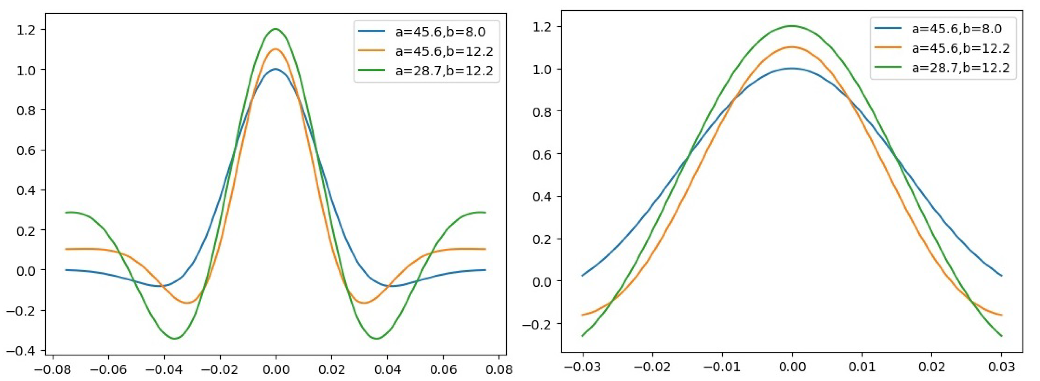
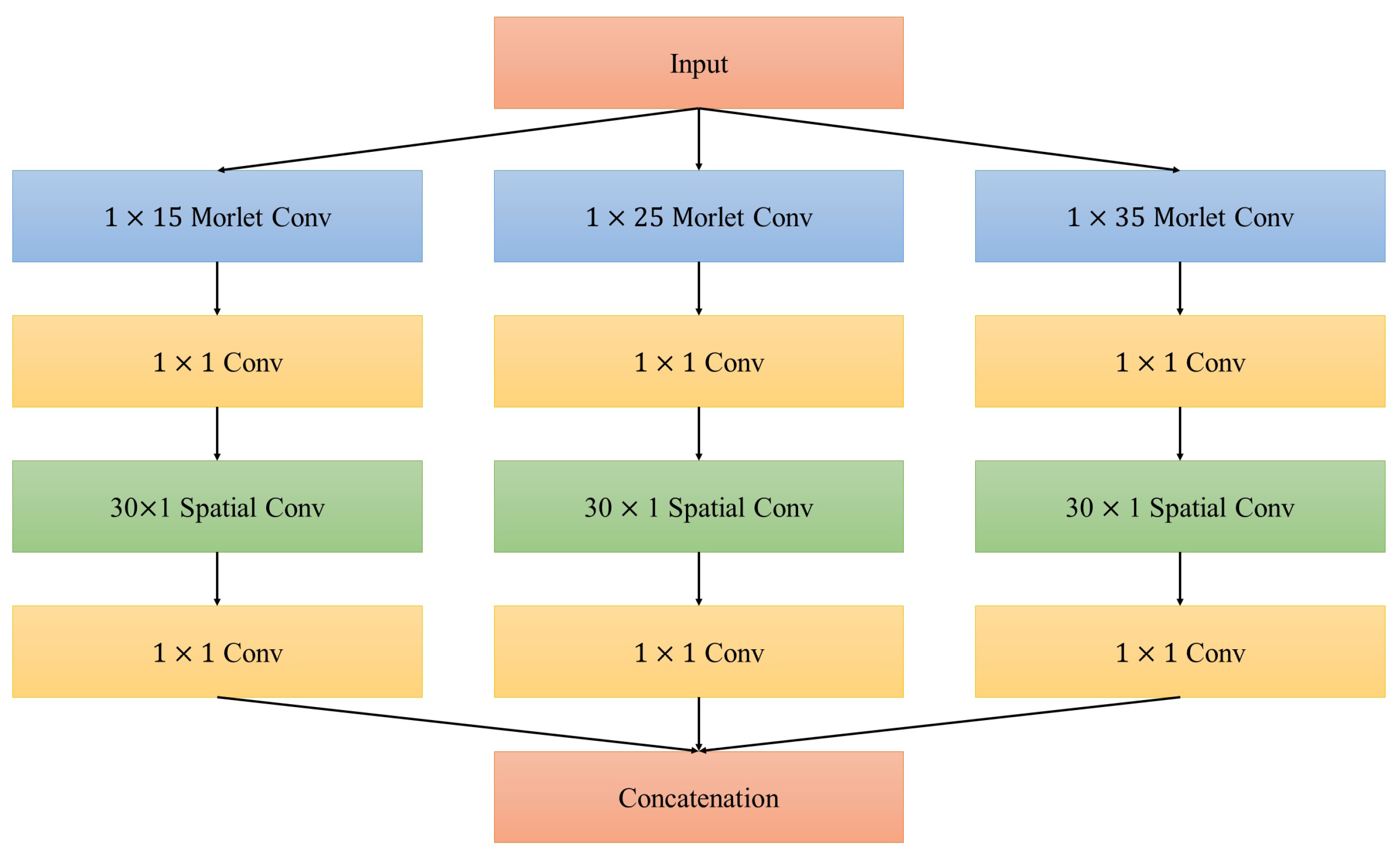
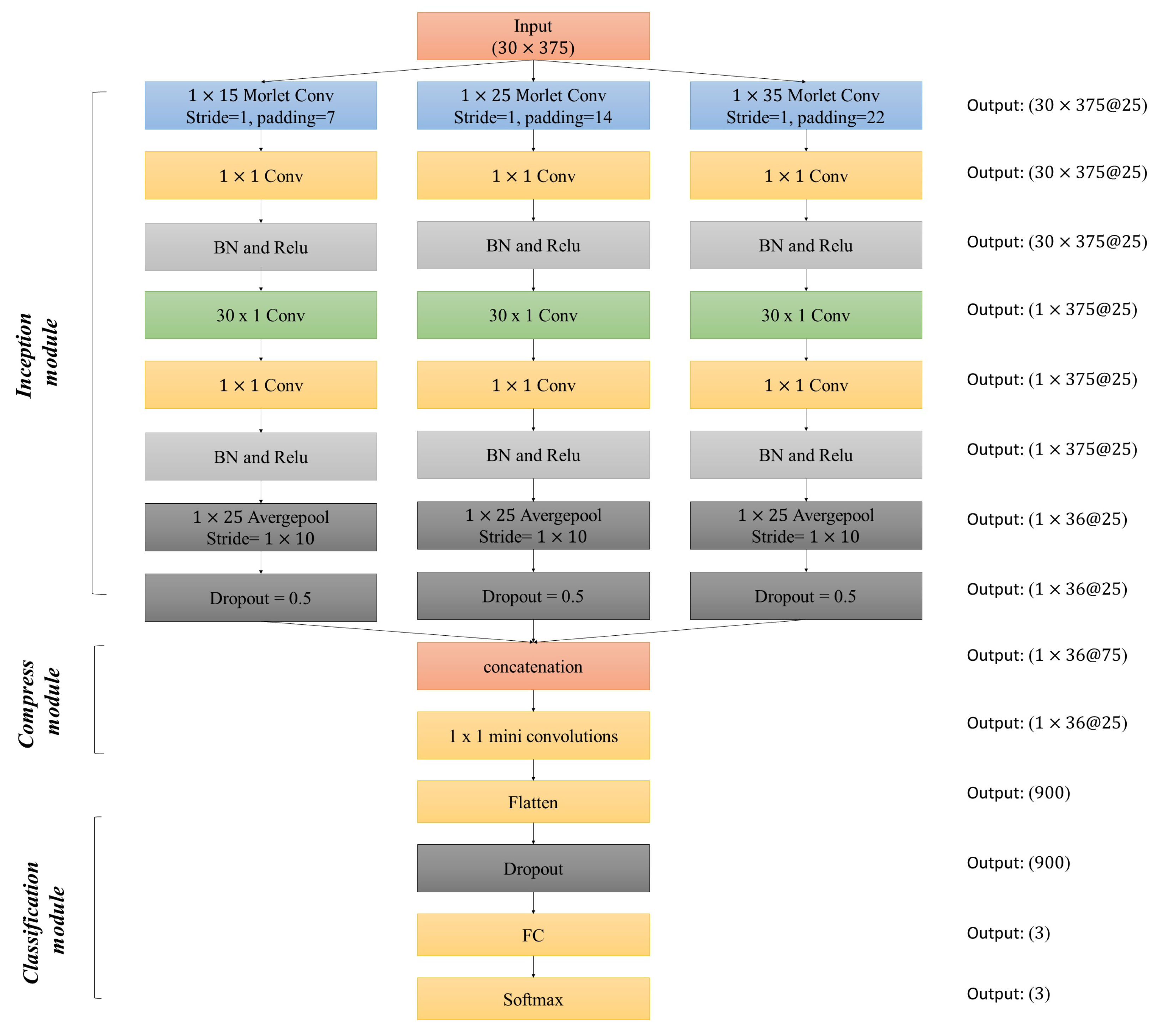
3.2. Architectural Details

Convolutional layers in the proposed model contains two convolutional layers, performing time convolution and spatial convolution respectively. Time-frequency convolutional layers extract the time-frequency features from input signals, while spatial convolutional layers explore the optimal spatial pattern of the extracted features. Both of them are 1D convolutional kernel.

We adopt morlet function as our convolutional kernel of time-frequency layers. As mentioned above, two parameters a and b are involved in this function, in which a controls the active time window of the wavelet kernel and b represents the central frequency (see Figure 1). Intuitively, a corresponds to the information of time domain and b corresponds to the information of frequency domain. Thus, the wavelet kernel is formulated as follows:

$$w_{\eta }^i=cos\left(2\pi b_{\eta }\frac{2i-kernel\_size}{2\ast srate}\right)e^{-\frac{1}{2}\ast a_{\eta }^2{\left(\frac{2i-kernel\_size}{2\ast srate}\right)}^2}$$

(2)

where $w_{\eta }^i$ denotes the i-th ($iϵ\left\{1,\dots ,kernel\_size\right\}$) element of the $\eta$-th convolutional kernel unit. $a_{\eta }$ and $b_{\eta }$ are the parameters controlling the pattern of $\eta$-th convolutional kernel. Since all convolutional kernels in the proposed model are 1D, scalar $kernel\_size$ denotes the convolutional kernel size. Scalar $srate$ denotes the sampling rate of the input EEG. It is important to note that a higher sampling rate means a shorter time window, which leads the model preferring the high-frequency components of the input. Figure 1 demonstrates the difference between morlet wave with the same parameters except for the sampling rate.

To capture multi-scale information in EEG signals, we apply inception module in the proposed network. Compared with stacked convolutional layer directly, inception architecture allows us keep information of each scale and find their optimal combinations. This is very useful when tackling with EEG data, since various events activate distinct brain regions in different timings and frequencies with different order. Correspondingly, their distinct features may be of various combinations of values extracted from different domains.

Each inception module contains two convolutional layers, performing time-frequency convolution and spatial convolution respectively. Time-frequency convolution layers extract time-frequency features of the input EEG, while spatial convolution layers search the optimal spatial pattern. Schirrmeister et. al. confirm the effectiveness of categories which divide the time-space features extraction layers into two independent 1D convolutional layers [13]. The divided category is quite similar with traditional analysis process and they believe it is the key to achieve improved performance. In this paper, we follow this design that dividing the features extraction layers into multi 1D convolutional layers in which joint time-frequency-space features can be extracted sequentially. Moreover, we insert a $1\times 1$ convolutional layer after the concatenation of multi-scale features to explore the optimal combinations of the extracted features [31].

Architecture of the inception module is illustrated in Figure 2. Note that all $1\times 1$ convolutional layers in the proposed model do not contain non-linear transformation (such as Relu function), since this layer is designed to search the optimal combinations of extracted features and we do not want to increase the complexity of the net any more. In addition, compared with traditional inception-based net in which a $1\times 1$ convolutional layer is always used as a compression method [30], the $1\times 1$ layer in our net does not compress the feature maps. The amount of $channe{l}_{i}n$ and $channe{l}_{o}ut$ is the same for the reason that EEG for various subjects are quite different and compression may degrade the generalization of the net.

3.3. Morletinceptionnet

Suppose that we were given an EEG data set (denoted by S), in which numbers of trials were contained. Each trial was a time-course EEG record belonging to one of several classes. Then the data set could be denoted by $S=\left\{\left(X_1,y_1\right),\left(X_2,y_2\right),\dots ,\left(X_N,y_N\right)\right\}$, where N represented the number of trials in the given data set S. Here, $X_i\in {\mathrm{R}}^{\mathrm{E}\times \mathrm{T}}$ was the input matrix with E denoting the number of electrodes and T representing the number of sample time points in each trial, while $y_i$ was the class label of the i-th trial. It takes values from a set of C class labels L ($L=\left\{l_1,l_2,\dots ,l_C\right\}$) corresponding to a set of brain activities. For example, $y_i$ in BCI competition IV 2a data sets could take class $l_1,l_2,l_3$ or $l_4$, meaning that during i-th trial of EEG, subjects performed either imagined left-hand movement, right-hand, foot movement, or tongue movement.

Inception module is designed to extracted multi-scale features by using various convolutional kernel size. Since information transmission process of each submodule (single column of inception module in Figure 3) is the same, we write the first submodule (kernel size is 15) for example. Given the $\eta$-th morlet kernel $W^{\eta }={\left\{w_1^{\eta },w_2^{\eta },\dots ,w_E^{\eta }\right\}}^T$, where $W^{\eta }\in R^{K\times E}$, K denotes the 1D kernel length and $w_e^{\eta }$ is generated by formulation (2), then we have:

$${\widehat{X}}_i=padding\left(X_i,7\right)$$

(3)

$$h_i^{\eta }=bia{s}^{\eta }+W^{\eta }\otimes {\widehat{X}}_i$$

(4)

where $X_i\in R^{\mathrm{ExT}}$ denotes the i-th trial of EEG. For the purposes of aligning the feature map size for different scales, we apply a padding function before the convolutional operation. The padding function fills seven zeros both in front of and rear of each row of $X_i$, and get ${\widehat{X}}_l\in R^{\mathrm{E}\times (\mathrm{T}+14)}$. $h_i^{\eta }$ corresponds to the $\eta$-th time-frequency feature map of the i-th EEG data, which is then as the input of the $1\times 1$ convolutional layer and the following Batch Normalization (BN) and Nonlinear Layer (Relu, $f(x)=max(x,0)$). After the processing of the two convolutional layers, the distribution of input may change and the shift of the data distribution would affect the training of the network [32].

Until now, the time-frequency features have been extracted and their optimal combinations are also calculated by a $1\times 1$ convolutional layer. The next step is to obtain the spatial pattern which corresponds to certain classes. The process of this step is same as the time-frequency step except for using CNN convolutional kernel instead of applying morlet kernel.

Following spatial convolution, the average pooling layer is utilized to aggregate the features of time dimension and transform the low-level features to high-level features. After that, a dropout layer which randomly discards a portion of the features with a certain probability is adopted to reduce the risk of overfitting.

Since three convolutional kernel sizes, which are $1\times 15$, $1\times 25$, and $1\times 35$, are involved in the MorletInceptionNet, three feature maps are generated by the Inception module. The purpose of the compression module is to integrate these feature maps together and then to transmit the integrated bigger sparse matrix into relatively dense submatrices. Feature maps are concatenated in depth first, and then compressed by a $1\times 1$ convolutional layer to generate a smaller dense matrix. Note that all outputs of the $1\times 1$ convolutional layer, including Inception module, are not transformed by the non-linear layer, since the involvement of $1\times 1$ convolutional layers is only for the optimization of feature combinations. We believe that although more non-linear layers gives the network a greater ability to represent the data, they also come with a higher overfitting risk.

The structure of the classification module is more straightforward compared with previous layers. The input is first flattened to a vector and then passed to a dropout layer in which features are discarded with a certain probability. After that, a dense layer is adopted to reduce the size of input vector to 3, which corresponds to the number of classes. Finally, SoftMax function is utilized to calculate the probability of given EEG trial for each class.

The proposed MorletInceptionNet is implemented on a workstation with Intel Xeon 2.4 GHz, 32 GB random access memory (RAM), and 8 GB DDR5 graphic card (NVidia GeForce GTX 1070) with 1920 CUDA cores using Python 3.6 and PyTorch deep learning library.

We perform a 5-fold cross validation on the training set in order to validate the proposed network and find optimal super-parameters using grid search. The convolutional layer parameters are first selected using cross-validation and then for testing on the test set. Configurations of MorletInceptionNet are illustrated in Figure 3 already, thus we will not give detailed descriptions again. We chose ADAM as the optimization method and the corresponding parameters are set to default values as [33]. The probability of the dropout layer is set to 50%. In addition, the weights of the morlet convolution a and b are randomly initialized by uniform distribution in U(1, 10) and U(3, 30), respectively.

4. Visual Fatigue Experiment

For the purpose of investigating the effective representations of fatigue states, we conducted a designed visual fatigue experiment to collect EEG data. Subject information, experiment protocol, and data recording and preprocessing were introduced as follow.

4.1. Subject

Twenty (mean age: 23 years; range: 22–25 years; 4 females; all right-handed) healthy students from the University of Chinese Academy of Sciences were recruited. Visual acuity and stereo acuity tests with autorefractometer and random dot stereogram (RDS) patterns were conducted to ensure all participants had normal vision. Subjects were required to refrain from antifatigue drinks or drowsiness-causing medications for 2 days before the experiment. Concurrently, they needed to keep reasonable rest with sleep durations of more than 7 h per night. They should comply with these regulations so as to join the study.

4.2. Experiment Protocol

In this study, 3D visual fatigue was induced by RDS with various disparities. The RDSs, which consisted of left-view and right-view, were generated by Unity 3D (Unity Technologies, St. Bellevue, WA, USA) and the dot density was 50 dots/deg${}^2$. The target area was shifted horizontally inwards or outwards to form crossed or uncrossed disparities. The shifts formed nine angular disparities of $0^{\circ },{0.3}^{\circ },-{0.3}^{\circ },{0.5}^{\circ },-{0.5}^{\circ },{0.9}^{\circ },-{0.9}^{\circ },{1.1}^{\circ }$, and $-{1.1}^{\circ }$ on the subject’s retina. When a subject was seated at a distance of 1020 mm (3 times of screen height), the target-area of RDS pattern was of ${1.24}^{\circ }\times {2.45}^{\circ }$ rectangular locating in the middle of the screen. A black point (0.1 radius) superimposed onto the middle of the pattern helped the subjects to fixate their eyes and prevented voluntary eye movements. The stimuli were presented via an AOC D2769Vh 3D display (27 inch, $1920\times 1024$ pixel resolution, and 60 Hz refresh rate, produced by Admiral Overseas Corporation, Wuhan, China) with subjects wearing polarized glasses sat in front of it.

Before the viewing task, subjects were asked to carry out a 2 min test to confirm all target disparities were identified clearly. Then they had a 5 min rest to adjust their status to a comfort level. The whole viewing task was divided into 6 blocks. Subjects were asked to finish a questionnaire to score their current visual fatigue states once a block was completed. The fatigue score ranged from 1 to 3, of which 1 meant no fatigue, 3 indicated extreme fatigue. Each block lasted for about 4.5 min, and RDSs of 9 disparities were presented in random order to simulate the real viewing condition. Additionally, the present times for each disparity were the same in one block (about 15 times for each disparity). The experimental environment was an office-like setting with an appropriate illumination condition of 300 lux without glare, which is the major cause of fatigue from lighting.

4.3. Data Recording and Preprocessing

Whole head EEG data were recorded from 34 channels. These channels were positioned based on the international standard 10–20 system and referenced to the left mastoids (A1). Four electrodes were used for recording the electrooculogram (EOG) activity and Thirty electrodes for the EEG activity. EEG data were recorded through the Compumedics NeuroScan Scan 4.5 software in tandem with the Synamps 2 system. EEG data were bandpass filtered (1–100 Hz) and digitized with a 24-bit analog to digital converter with a sampling rate of 1000 Hz. Electrode impedance at each electrode was maintained below 10 $\mathrm{k}\mathsf{\Omega }$.

One subject was excluded for poor signal quality, the rest raw EEG data from all six blocks were appended to create one dataset for each subject and then resampled to 250 Hz to reduce the computational requirements of further processing steps. After that, the EEG datasets were band-pass filtered into 1–40 Hz with a Parks McClellan notch filter at 50 Hz, and a common average reference was computed from all the channels. In addition, artifact subspace reconstruction (ASR) [34], implemented as a plug-in to the EEGLAB, was applied using a threshold ($\sigma =20$) to reduce data contamination by high-amplitude artifacts.

Thereafter, a trial of epoch of 1500 ms (ranging from −500 to +1000 ms around zero, which corresponded to stimulus onset) were extracted from continuous EEG data.

After this step, there were about 1200 trials for each of 19 subjects, of which the number of each fatigue level was about 400. For each trial, we got a matrix with the shape of $30\times 375$ (channels × sampling points). Finally, we get the fatigue data set with size of $19\times 1200\times 30\times 375$ ($subjects\times trials\times channels\times timingsamples$). We perform a five-fold cross validation in order to select parameters. The whole shuffled set is divided into two separate sets, training set and testing set, with the proportion of 0.8 and 0.2. Cross-validation is conducted on the training set and then the test is run on the test set.

5. Results

To validate the performance of the proposed network, we make a comparison with the state-of-the-art methods to prove the effectiveness of our model. In this section, we first give a brief introduction of the baseline methods. Then the comparisons between our model and baseline methods are made. Finally, the learned representation is visualized to understand how the model achieves such performance.

5.1. Baseline Methods and Performance Metrics

The baseline methods are listed as follows:

• CNNInceptionNet: Replace the morlet layer in the proposed MorletInceptionNet with regular convolutional lay to validate the effectiveness of the morlet kernel.
• Shallow ConvNet [13]: Inspired by FBCSP algorithm, Shallow ConvNet extract features in a similar way. But Shallow ConvNet uses a convolutional neural network to do all the computations and all the steps are optimized in an end-to-end manner.
• Deep ConvNet [13]: It has four convolution-pooling blocks and is much deeper than Shallow ConvNet.
• EEGNet [15]: It has two convolution-pooling blocks. The difference between EEGNet and ConvNets introduced above is that EEGNet uses depth-wise and separable convolution.
• MorletNet: Replace the first layer of Shallow ConvNet with morlet layer. The sub-architecture of inception module proposed in this paper is similar with Shallow ConvNet. This network is used to validate the effectiveness of morlet kernel by comparing with Shallow ConvNet, as well as the effectiveness of proposed inception architecture by comparing with MorletInceptionNet.
• FBCSP-SVM [23]: A traditional augmented-CSP algorithm using overlapping frequency bands. The log-energy features are extracted for each frequency band in spatial transformed EEG signal. The extracted features are then passed into SVM for classification. We adopt one-vs-rest strategy for multi-class classification.
• 2DRCNN [16]: It has 3 stacked convolutional layers to extract spatial information and then the feature maps are passed into a single LSTM layer with 32 memory cells to extract temporal information in EEG.

In this paper, kappa value $k=\left(p_a-p_c\right)/\left(1-p_c\right)$ is used as one of the evaluation metrics to assess the performance of the classifiers, where $p_a$ is the proportion of the successful classification (identical to accuracy) and $p_c$ is the proportion of random classification [28].

5.2. Classification Performances

The proposed MorletInceptionNet is trained to detect visual fatigue status on both subject-specific and cross-subject datasets. The network performances are obtained on each dataset by 5-fold cross validation. For each dataset, 60% of the samples are randomly selected as training set, while 20% is randomly selected as validation set, and the remaining 20% is reserved as testing set. We adopt the grid search to find the optimal super-parameters for all algorithms.

First of all, parameters numbers for various models are calculated and are summarized in

Table 1. Numbers of parameters in various models.

Net	Number of Parameters
CNNInceptionNet	67,078
Shallow ConvNet	51,403
Deep ConvNet	163,478
EEGNet	2115
MorletNet	54,703
2DRCNN	over 130,000,000
MorletInceptionNet	65,278

. Then the performances of models on the subject-specific an cross-subject dataset in terms of k value and accuracy are list in

Table 2. Comparison of our method with baseline methods in terms of $kappa$ value for the fatigue dataset of specific subject and cross-subject, best scores are in bold.

Subject	Deep4 ConvNet	EEGNet4	Shallow ConvNet	MorletNet	MorletInceptionNet	CNNInceptionNet	FBCSP-SVM	2DRCNN
s1	0.21 ± 0.03	0.20 ± 0.04	0.33 ± 0.06	0.40 ± 0.04	0.41 ± 0.05	0.39 ± 0.06	0.36 ± 0.04	0.30 ± 0.03
s2	0.15 ± 0.03	0.42 ± 0.05	0.51 ± 0.06	0.55 ± 0.08	0.54 ± 0.02	0.53 ± 0.06	0.52 ± 0.05	0.46 ± 0.04
s3	0.72 ± 0.05	0.73 ± 0.09	0.71 ± 0.03	0.72 ± 0.05	0.76 ± 0.04	0.76 ± 0.04	0.71 ± 0.03	0.68 ± 0.05
s4	0.32 ± 0.02	0.33 ± 0.08	0.46 ± 0.02	0.54 ± 0.06	0.52 ± 0.04	0.52 ± 0.03	0.48 ± 0.03	0.46 ± 0.02
s5	0.26 ± 0.08	0.37 ± 0.06	0.54 ± 0.04	0.48 ± 0.06	0.50 ± 0.04	0.52 ± 0.05	0.51 ± 0.04	0.43 ± 0.04
s6	0.07 ± 0.05	0.10 ± 0.07	0.30 ± 0.02	0.24 ± 0.08	0.32 ± 0.05	0.30 ± 0.07	0.30 ± 0.02	0.26 ± 0.05
s7	0.25 ± 0.08	0.26 ± 0.09	0.50 ± 0.05	0.42 ± 0.07	0.45 ± 0.09	0.41 ± 0.07	0.48 ± 0.03	0.39 ± 0.04
s8	0.10 ± 0.07	0.29 ± 0.05	0.43 ± 0.13	0.38 ± 0.05	0.44 ± 0.05	0.44 ± 0.07	0.41 ± 0.04	0.36 ± 0.06
s9	0.09 ± 0.02	0.18 ± 0.02	0.25 ± 0.03	0.27 ± 0.07	0.28 ± 0.07	0.27 ± 0.05	0.27 ± 0.05	0.19 ± 0.04
s10	0.20 ± 0.04	0.17 ± 0.13	0.28 ± 0.08	0.29 ± 0.10	0.31 ± 0.09	0.30 ± 0.09	0.30 ± 0.06	0.29 ± 0.07
s11	0.55 ± 0.10	0.55 ± 0.09	0.44 ± 0.14	0.44 ± 0.06	0.52 ± 0.08	0.52 ± 0.10	0.48 ± 0.03	0.45 ± 0.03
s12	0.01 ± 0.03	0.01 ± 0.06	0.04 ± 0.04	0.10 ± 0.05	0.18 ± 0.10	0.13 ± 0.08	0.15 ± 0.09	0.16 ± 0.04
s13	0.27 ± 0.03	0.41 ± 0.07	0.52 ± 0.05	0.55 ± 0.07	0.58 ± 0.04	0.52 ± 0.03	0.56 ± 0.04	0.47 ± 0.04
s14	0.17 ± 0.06	0.19 ± 0.05	0.51 ± 0.04	0.47 ± 0.05	0.52 ± 0.05	0.49 ± 0.05	0.50 ± 0.05	0.46 ± 0.05
s15	0.46 ± 0.10	0.40 ± 0.06	0.47 ± 0.05	0.49 ± 0.08	0.51 ± 0.09	0.51 ± 0.04	0.47 ± 0.04	0.44 ± 0.03
s16	0.34 ± 0.07	0.35 ± 0.08	0.45 ± 0.05	0.46 ± 0.01	0.42 ± 0.05	0.47 ± 0.02	0.41 ± 0.01	0.36 ± 0.01
AVG	0.26 ± 0.05	0.31 ± 0.07	0.42 ± 0.06	0.43 ± 0.06	0.45 ± 0.06	0.44 ± 0.06	0.43 ± 0.04	0.38 ± 0.04
Cross-subject	0.31 ± 0.04	0.35 ± 0.05	0.50 ± 0.05	0.50 ± 0.04	0.61 ± 0.06	0.57 ± 0.07	0.52 ± 0.05	0.48 ± 0.06

and

Table 3. Comparison of our method with baseline methods in terms of accuracy for the fatigue dataset for each subject and cross-subject, best scores are in bold.

Subject	Deep4 ConvNet	EEGNet4	Shallow ConvNet	MorletNet	MorletInceptionNet	CNNInceptionNet	FBCSP-SVM	2DRCNN
s1	0.42 ± 0.02	0.45 ± 0.02	0.58 ± 0.02	0.65 ± 0.01	0.63 ± 0.03	0.62 ± 0.03	0.57 ± 0.02	0.48 ± 0.03
s2	0.39 ± 0.05	0.63 ± 0.01	0.76 ± 0.03	0.78 ± 0.01	0.77 ± 0.02	0.79 ± 0.02	0.73 ± 0.02	0.64 ± 0.01
s3	0.84 ± 0.01	0.86 ± 0.02	0.86 ± 0.02	0.85 ± 0.02	0.86 ± 0.02	0.86 ± 0.00	0.84 ± 0.01	0.84 ± 0.02
s4	0.54 ± 0.03	0.53 ± 0.02	0.66 ± 0.01	0.69 ± 0.02	0.71 ± 0.02	0.69 ± 0.02	0.54 ± 0.03	0.51 ± 0.02
s5	0.56 ± 0.04	0.57 ± 0.05	0.70 ± 0.01	0.69 ± 0.02	0.73 ± 0.02	0.71 ± 0.01	0.71 ± 0.02	0.69 ± 0.02
s6	0.51 ± 0.02	0.53 ± 0.04	0.67 ± 0.01	0.63 ± 0.03	0.63 ± 0.03	0.59 ± 0.04	0.63 ± 0.01	0.58 ± 0.01
s7	0.64 ± 0.04	0.65 ± 0.03	0.78 ± 0.01	0.74 ± 0.02	0.74 ± 0.01	0.74 ± 0.02	0.74 ± 0.02	0.65 ± 0.03
s8	0.84 ± 0.01	0.84 ± 0.02	0.87 ± 0.02	0.86 ± 0.02	0.88 ± 0.02	0.87 ± 0.02	0.85 ± 0.02	0.85 ± 0.03
s9	0.52 ± 0.02	0.48 ± 0.03	0.58 ± 0.01	0.58 ± 0.02	0.62 ± 0.01	0.59 ± 0.02	0.58 ± 0.04	0.53 ± 0.04
s10	0.75 ± 0.02	0.74 ± 0.04	0.86 ± 0.01	0.85 ± 0.01	0.85 ± 0.02	0.85 ± 0.01	0.76 ± 0.02	0.82 ± 0.01
s11	0.88 ± 0.05	0.90 ± 0.01	0.89 ± 0.01	0.86 ± 0.01	0.88 ± 0.02	0.90 ± 0.02	0.84 ± 0.05	0.88 ± 0.02
s12	0.59 ± 0.02	0.58 ± 0.02	0.68 ± 0.01	0.74 ± 0.02	0.74 ± 0.01	0.74 ± 0.02	0.74 ± 0.02	0.73 ± 0.01
s13	0.50 ± 0.03	0.56 ± 0.02	0.63 ± 0.02	0.65 ± 0.01	0.69 ± 0.03	0.63 ± 0.03	0.65 ± 0.02	0.63 ± 0.02
s14	0.41 ± 0.03	0.46 ± 0.03	0.67 ± 0.03	0.67 ± 0.02	0.68 ± 0.01	0.67 ± 0.02	0.66 ± 0.01	0.64 ± 0.02
s15	0.79 ± 0.01	0.71 ± 0.03	0.77 ± 0.01	0.78 ± 0.02	0.80 ± 0.01	0.80 ± 0.02	0.77 ± 0.03	0.77 ± 0.02
s16	0.56 ± 0.03	0.59 ± 0.07	0.63 ± 0.03	0.64 ± 0.01	0.69 ± 0.01	0.65 ± 0.02	0.65 ± 0.02	0.62 ± 0.04
AVG	0.61 ± 0.03	0.63 ± 0.03	0.73 ± 0.02	0.73 ± 0.01	0.74 ± 0.02	0.73 ± 0.02	0.70 ± 0.02	0.67 ± 0.02
Cross-subject	0.67 ± 0.02	0.68 ± 0.02	0.73 ± 0.04	0.71 ± 0.02	0.74 ± 0.03	0.72 ± 0.03	0.73 ± 0.03	0.71 ± 0.02

respectively. Overall, all methods achieve acceptable performances on most subjects. The undesirable kappa values observed on s6, s9, s10, s12 originated from the severely unbalanced class. The proposed MorletInceptionNet achieves the best performance compared with other baseline methods for most subjects in both kappa value (p = 0.01, Wilcoxon signed-rank test) and accuracy (p = 0.017, Wilcoxon signed-rank test). According to the average kappa value in Table 2, the proposed MorletInceptionNet reaches 0.45, which exceeds the state-of-the-art methods by 0.03. This suggests the effectiveness of the proposed architecture.

To validate the whether the morlet kernel and inception architecture are helpful for improving performance, two architectural networks (CNNInceptionNet and MorletNet) are involved to demonstrate the effectiveness of the proposed architectures. On one hand, we replace the morlet layer with regular convolutional layer to test whether the performance is improved due to the morlet kernel. On another hand, we replace the multi-scaling architecture with one, which can be viewed as Shallow ConvNet with morlet layer, to test whether the improvement is caused by proposed inception architecture. Statistical results from the comparison between kappa value of MorletInceptionNet and CNNInceptionNet suggest a significant improvement of performance by the adoption of morlet kernel (p = 0.049, Wilcoxon signed-rank test). Moreover, the comparison between the kappa values of MorletInceptionNet and MorletNet also implies a significant improvement of performance by adoption of inception module (p = 0.007, Wilcoxon signed-rank test). These statistical results confirm the effectiveness of the proposed architecture. Comparison between MorletNet and Shallow ConvNet is also conducted and the insignificant statistical result (p = 0.31 Wilcoxon signed-rank test) suggests the replacement of timing layer using morlet kernel is maybe not effective for the architecture of Shallow ConvNet. These imply that although morlet convolution can reduce the number of parameters (see Table 1), structural optimization of the Net is also needed.

Both Deep ConvNet and 2DRCNN achieved the worst results in most subjects, showing increasing the depth of network may be not helpful for classification tasks. The magnitude of parameters in these two models is much larger than the rest, especially for 2DRCNN there are over 100 million parameters (Table 1). These provide evidence for the hypothesis mentioned above that increasing the depth of the model may be not helpful for EEG-based classification tasks. However, a very small amount of parameters seems to not be helpful as well. EEGNet, which only has about 2115 parameters, achieves the second worst results (Table 1). Shallow ConvNet, as we know, is a 4 layers-net consisting of one timing layer and one spatial layer which extracts timing and spatial features consequently. This compact architecture with a smaller magnitude of parameters compared with Deep ConvNet outperforms other baseline methods (while not for the proposed methods), which proves its effectiveness. Compared with MorletNet, replacement of the timing layer in Shallow ConvNet using morlet kernel without structural optimization may be not helpful for performance improvement (p = 0.31 Wilcoxon signed-rank test), additional structural optimization is also needed.

For a traditional baseline method, FBCSP-SVM is very competitive as an universal model in various EEG-based classification tasks. In our experiment, FBCSP-SVM achieves the second best performance both in $kappa$ and classification accuracy. This implies that both frequency domain and space domain features are effective in visual fatigue classification tasks, which is consistent with previous research [18,19,20]. This also proves the effectiveness of the proposed model in which space-frequency-time features are extracted for classification.

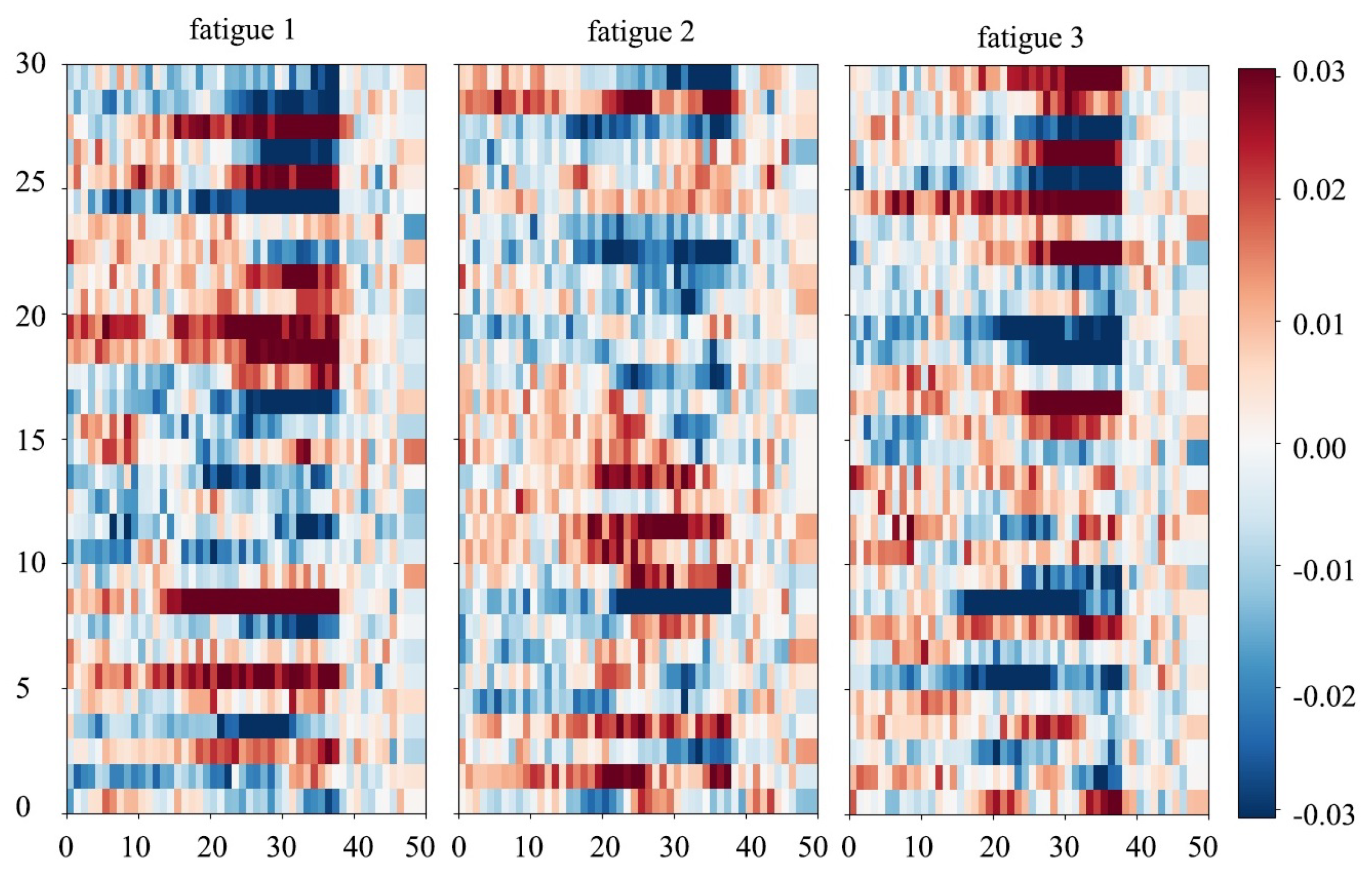
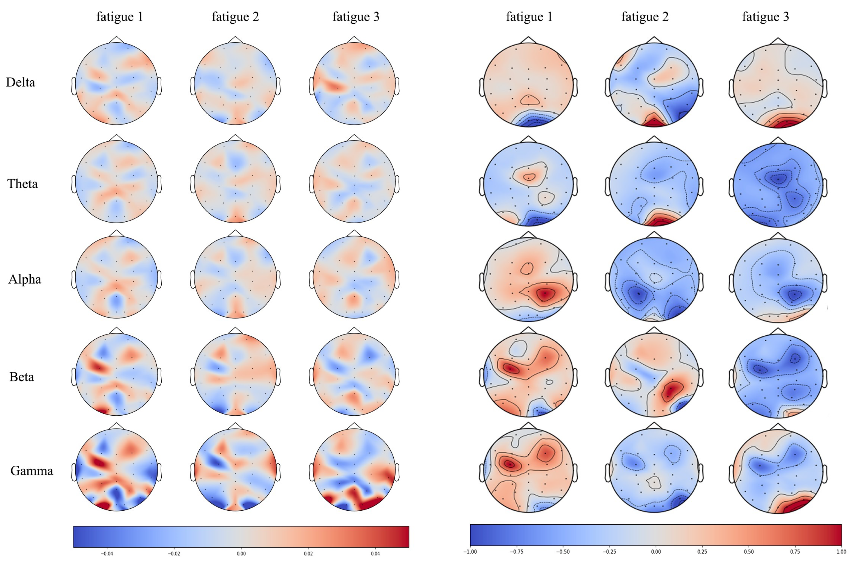
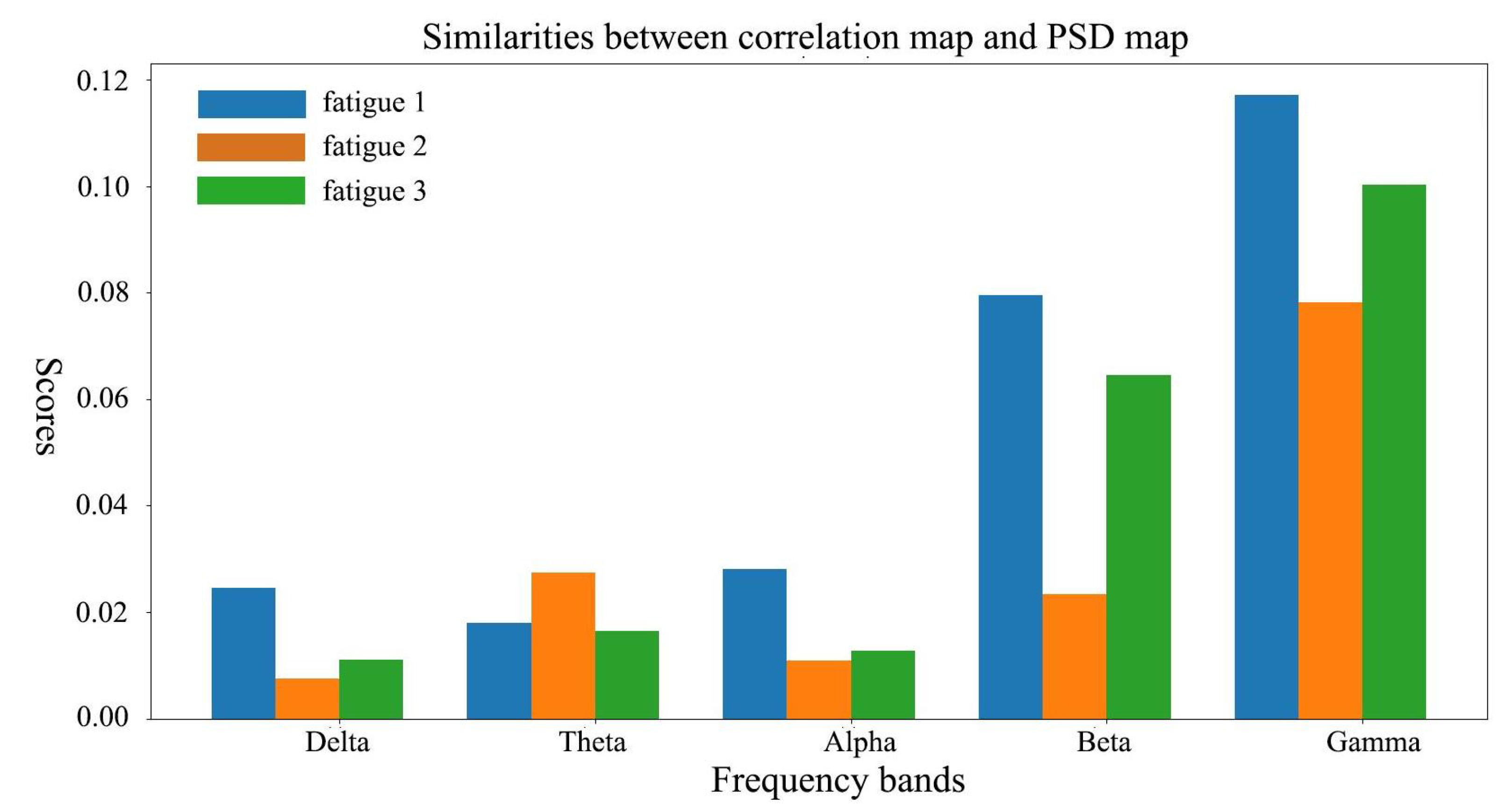
5.3. Visualizing the Learned Representation

To understand the reason why the proposed method outperforms baseline methods, we make use of Input-perturbation network-prediction correlation maps, which were proposed by Schisstmeter [13], to investigate what our model has learned. In his method, a small perturbation in a certain frequency band is added into the input signal, then the correlations between changes of input and output are calculated. In this paper, only the outputs of dense layer (before SoftMax unit) are utilized as the model output to compute the correlation maps, since outputs of these can reflect the final classification results directly and the values of this layers are continuous which is convenient for the correlation computation.

Since all subjects have similar correlation value, in this paper we select subject 12 for example. The results are shown in Figure 4, which suggest that most higher correlations (deep red or deep blue in the Figure 4) exist in the frequency interval of 15–40 Hz, which corresponds to $\beta$ band and $\gamma$ band. Since deep red and blue imply strong positive and negative correlation between input and dense layer output respectively, Figure 4 implies that the trained model is more sensitive to perturbation in frequency bands of 15–40 Hz. This is consistent with previous researches, in which the PSD in $\beta$ band has been found of a statistical relationship with 3D visual fatigue [10,18,20,21]. In addition, we can also observe that most correlated electrodes are located in the parietal-occipital area. This is also consistent with previous studies, in which parietal-occipital area, especially occipital, play an important role in the 3D visual system [35] and their activity always vary significantly when subjects suffer visual fatigue [18,36,37]. Results indicate that the proposed model indeed has learned frequency-space representations of EEG.

Interestingly, our model is also found to be sensitive to the perturbation in the $\gamma$ band, which has been hardly mentioned in previous researches. To validate whether the corresponding PSD is effective for visual fatigue classification in our dataset, we conduct a one-way repeated measurement ANOVA to investigate the relationship between PSD in $\gamma$ band and visual fatigue levels. Statistical results reveal the $\gamma$ PSD in electrodes located at parietal-occipital area such as 22 (F(2, 36) = 4.237, p = 0.022), 25 (F(2, 36) = 4.918, p = 0.013), 27 (F(2, 36) = 6.447, p = 0.004), 29 (F(2, 36) = 3.487, p = 0.041), 30 (F(2, 36) = 3.279, p = 0.049) vary significantly with the visual fatigue. This is consistent with the results demonstrated in Figure 4.

Since we have demonstrated that our model has learned the frequency domain information in EEG, here we further investigate the spatial relationship between learned representations and PSD features. Each topographic map of correlation values (Figure 5, left) can be viewed as one distinct spatial pattern of features and deeper colors in the map imply the corresponding areas are more important for classification. For the consideration of compatibility, difference between PSDs of certain fatigue level and the rests are calculated for comparison with correlation value. Topographic maps of both correlation values (Figure 5, left) and PSD difference (Figure 5, right) are presented in Figure 5. In topographic maps of correlation values, we can obviously observe the color is going deep with frequency increasing from $\delta$ to $\gamma$, which implies components of higher frequency ($\beta$ and $\gamma$ band) in EEG play more important roles in the proposed model. Interestingly, their spatial pattern is quite similar with the pattern of PSD in the corresponding frequency band. To compare their spatial similarities quantitatively, for each fatigue level and frequency band, we compute the cross product as representation of similarity and the results are demonstrated in Figure 6. We can observe clearly that the dramatic increasing in $\beta$ and $\gamma$ band in Figure 6, this implies it is likely that the proposed net has learned the joint space-frequency features of the high frequency band.

6. Conclusions

In this paper, we conduct a designed experiment to collect raw EEG signals of various fatigue levels as the dataset, and then present a multi-scale convolutional neural network (CNN) architecture named MorletInceptionNet to detect visual fatigue using EEG as input, which exploits the spatial-temporal structure of multichannel EEG signals. Five competitive methods are also involved to validate the effectiveness of the proposed MorletInceptionNet on our visual fatigue dataset. Results demonstrate that our model achieve overall the best performance for two widely used evaluation metrics, i.e., classification accuracy and kappa value. Through visualizing the learned representation, we demonstrate that our model can learn the joint time-frequency-space features to distinguish fatigue levels automatically. Though our method achieves promising results, our method can be improved in future work. Firstly, compared to traditional convolutional kernel, morlet kernel need more computational resources and the time cost in computation increases about 33% (from 3 h to 4 h for 200 iterations). We believe finding alternative approximation algorithms for exp and cos operators will be helpful for reducing the computational resources. Secondly, results from visualization suggest that our model is not sensitive to perturbations from $\alpha$ bands, which is considered as one of the main indicators of visual fatigue evaluation. This implies that although the proposed model indeed achieves the best performance, there are still effective features that have not been learned. These issues require more studies in future work.

References

1. Lambooij, M.; Fortuin, M.; Heynderickx, I.; IJsselsteijn, W. Visual discomfort and visual fatigue of stereoscopic displays: A review. J. Imaging Sci. Technol. 2009, 53, 30201-1–30201-14. [Google Scholar] [CrossRef]
2. Zhang, L.; Ren, J.; Xu, L.; Qiu, X.J.; Jonas, J.B. Visual comfort and fatigue when watching three-dimensional displays as measured by eye movement analysis. Br. J. Ophthalmol. 2013, 97, 941–942. [Google Scholar] [CrossRef] [PubMed]
3. Wook Wee, S.; Moon, N.J. Clinical evaluation of accommodation and ocular surface stability relavant to visual asthenopia with 3D displays. BMC Ophthalmol. 2014, 14, 29. [Google Scholar]
4. Neveu, P.; Roumes, C.; Philippe, M.; Fuchs, P.; Priot, A.E. Stereoscopic Viewing Can Induce Changes in the CA/C Ratio. Investig. Ophthalmol. Vis. Sci. 2016, 57, 4321–4326. [Google Scholar] [CrossRef] [Green Version]
5. Yu, J.H.; Lee, B.H.; Kim, D.H. EOG based eye movement measure of visual fatigue caused by 2D and 3D displays. In Proceedings of the 2012 IEEE-EMBS International Conference on Biomedical and Health Informatics, Hong Kong, China, 5–7 January 2012; pp. 305–308. [Google Scholar]
6. Park, S.; Won, M.J.; Mun, S.; Lee, E.C.; Whang, M. Does visual fatigue from 3D displays affect autonomic regulation and heart rhythm. Int. J. Psychophysiol. 2014, 92, 42–48. [Google Scholar] [CrossRef]
7. Park, S.; Won, M.J.; Lee, E.C.; Mun, S.; Park, M.C.; Whang, M. Evaluation of 3D cognitive fatigue using heart–brain synchronization. Int. J. Psychophysiol. 2015, 97, 120–130. [Google Scholar] [CrossRef]
8. Ma, X.; Huang, X.; Shen, Y.; Qin, Z.; Ge, Y.; Chen, Y.; Ning, X. EEG based topography analysis in string recognition task. Phys. A Stat. Mech. Its Appl. 2017, 469, 531–539. [Google Scholar] [CrossRef]
9. Sanei, S.; Chambers, J.A. EEG Signal Processing; John Wiley Sons, Ltd.: Hoboken, NJ, USA, 2007; pp. 127–156. [Google Scholar]
10. Chen, C.; Li, K.; Wu, Q.; Wang, H.; Qian, Z.; Sudlow, G. EEG-based detection and evaluation of fatigue caused by watching 3DTV. Displays 2013, 34, 81–88. [Google Scholar] [CrossRef]
11. He, K.; Gkioxari, G.; Dollár, P.; Girshick, R. Mask r-cnn. In Proceedings of the IEEE International Conference on Computer Vision, Venice, Italy, 22–29 October 2017; pp. 2961–2969. [Google Scholar]
12. Abdel-Hamid, O.; Mohamed, A.R.; Jiang, H.; Deng, L.; Penn, G.; Yu, D. Convolutional neural networks for speech recognition. IEEE/ACM Trans. Audio Speech Lang. Process. 2014, 22, 1533–1545. [Google Scholar] [CrossRef]
13. Schirrmeister, R.T.; Springenberg, J.T.; Fiederer, L.D.J.; Glasstetter, M.; Eggensperger, K.; Tangermann, M.; Hutter, F.; Burgard, W.; Ball, T. Deep learning with convolutional neural networks for EEG decoding and visualization. Hum. Brain Mapp. 2017, 38, 5391–5420. [Google Scholar] [CrossRef] [Green Version]
14. Zhang, D.; Yao, L.; Chen, K.; Wang, S.; Chang, X.; Liu, Y. Making Sense of Spatio-Temporal Preserving Representations for EEG-Based Human Intention Recognition. IEEE Trans. Cybern. 2019. [Google Scholar] [CrossRef] [PubMed]
15. Lawhern, V.J.; Solon, A.J.; Waytowich, N.R.; Gordon, S.M.; Hung, C.P.; Lance, B.J. EEGNet: A compact convolutional neural network for EEG-based brain–computer interfaces. J. Neural Eng. 2018, 15, 056013. [Google Scholar] [CrossRef] [PubMed]
16. Maddula, R.; Stivers, J.; Mousavi, M.; Ravindran, S.; de Sa, V. Deep Recurrent Convolutional Neural Networks for Classifying P300 BCI signals. In Proceedings of the 7th Graz Brain-Computer Interface Conference (GBCIC 2017), Graz, Austria, 18–22 September 2017. [Google Scholar]
17. Bashivan, P.; Rish, I.; Yeasin, M.; Codella, N. Learning representations from EEG with deep recurrent-convolutional neural networks. arXiv 2015, arXiv:1511.06448. [Google Scholar]
18. Kim, Y.J.; Lee, E.C. EEG based comparative measurement of visual fatigue caused by 2D and 3D displays. In Proceedings of the International Conference on Human-Computer Interaction, Orlando, FL, USA, 9–14 July 2011; Springer: Berlin/Heidelberg, Germany, 2011; pp. 289–292. [Google Scholar]
19. Yin, J.; Jin, J.; Liu, Z.; Yin, T. Preliminary study on EEG-based analysis of discomfort caused by watching 3D images. In Advances in Cognitive Neurodynamics (IV); Springer: Dordrecht, The Netherlands, 2015; pp. 329–335. [Google Scholar]
20. Guo, M.; Liu, Y.; Zou, B.; Wang, Y. Study of electroencephalography-based objective stereoscopic visual fatigue evaluation. In Proceedings of the 2015 International Symposium on Bioelectronics and Bioinformatics (ISBB), Beijing, China, 14–17 October 2015; pp. 160–163. [Google Scholar]
21. Hsu, B.W.; Wang, M.J.J. Evaluating the effectiveness of using electroencephalogram power indices to measure visual fatigue. Percept. Motor Skills 2013, 116, 235–252. [Google Scholar] [CrossRef] [PubMed]
22. Ramoser, H.; Muller-Gerking, J.; Pfurtscheller, G. Optimal spatial filtering of single trial EEG during imagined hand movement. IEEE Trans. Rehabil. Eng. 2000, 8, 441–446. [Google Scholar] [CrossRef] [PubMed]
23. Yang, H.; Sakhavi, S.; Ang, K.K.; Guan, C. On the use of convolutional neural networks and augmented CSP features for multi-class motor imagery of EEG signals classification. In Proceedings of the 2015 37th Annual International Conference of the IEEE Engineering in Medicine and Biology Society (EMBC), Milan, Italy, 25–29 August 2015; pp. 2620–2623. [Google Scholar]
24. Croce, P.; Zappasodi, F.; Marzetti, L.; Merla, A.; Pizzella, V.; Chiarelli, A.M. Deep Convolutional Neural Networks for feature-less automatic classification of Independent Components in multi-channel electrophysiological brain recordings. IEEE Trans. Biomed. Eng. 2018. [Google Scholar] [CrossRef]
25. Chiarelli, A.M.; Croce, P.; Merla, A.; Zappasodi, F. Deep learning for hybrid EEG-fNIRS brain–computer interface: Application to motor imagery classification. J. Neural Eng. 2018, 15, 036028. [Google Scholar] [CrossRef]
26. Emami, A.; Kunii, N.; Matsuo, T.; Shinozaki, T.; Kawai, K.; Takahashi, H. Seizure detection by convolutional neural network-based analysis of scalp electroencephalography plot images. NeuroImage Clin. 2019, 22, 101684. [Google Scholar] [CrossRef]
27. Fahimi, F.; Zhang, Z.; Goh, W.B.; Lee, T.S.; Ang, K.K.; Guan, C. Inter-subject transfer learning with end-to-end deep convolutional neural network for EEG-based BCI. J. Neural Eng. 2019, 16, 2. [Google Scholar] [CrossRef]
28. Zhao, D.; Tang, F.; Si, B.; Feng, X. Learning joint space–time–frequency features for EEG decoding on small labeled data. Neural Netw. 2019, 114, 67–77. [Google Scholar] [CrossRef]
29. Szegedy, C.; Vanhoucke, V.; Ioffe, S.; Shlens, J.; Wojna, Z. Rethinking the inception architecture for computer vision. In Proceedings of the IEEE Conference on Computer Vision and Pattern Recognition, Las Vegas, NV, USA, 26–30 June 2016; pp. 2818–2826. [Google Scholar]
30. Szegedy, C.; Liu, W.; Jia, Y.; Sermanet, P.; Reed, S.; Anguelov, D.; Erhan, D.; Vanhoucke, V.; Rabinovich, A. Going deeper with convolutions. In Proceedings of the IEEE Conference on Computer Vision and Pattern Recognition, Boston, MA, USA, 7–12 June 2015; pp. 1–9. [Google Scholar]
31. Lin, M.; Chen, Q.; Yan, S. Network in network. arXiv 2013, arXiv:1312.4400. [Google Scholar]
32. Ioffe, S.; Szegedy, C. Batch normalization: Accelerating deep network training by reducing internal covariate shift. arXiv 2015, arXiv:1502.03167. [Google Scholar]
33. Kingma, D.P.; Ba, J. Adam: A method for stochastic optimization. arXiv 2014, arXiv:1412.6980. [Google Scholar]
34. Mullen, T.R.; Kothe, C.A.; Chi, Y.M.; Ojeda, A.; Kerth, T.; Makeig, S.; Jung, T.P.; Cauwenberghs, G. Real-time neuroimaging and cognitive monitoring using wearable dry EEG. IEEE Trans. Biomed. Eng. 2015, 62, 2553–2567. [Google Scholar] [CrossRef] [PubMed]
35. Kravitz, D.J.; Saleem, K.S.; Baker, C.I.; Mishkin, M. A new neural framework for visuospatial processing. Nat. Rev. Neurosci. 2011, 12, 217. [Google Scholar] [CrossRef] [PubMed]
36. Chen, C.; Wang, J.; Liu, Y.; Chen, X. Using Bold-fMRI to detect cortical areas and visual fatigue related to stereoscopic vision. Displays 2017, 50, 14–20. [Google Scholar] [CrossRef]
37. Kim, D.; Jung, Y.J.; Han, Y.J.; Choi, J.; Kim, E.W.; Jeong, B.; Ro, Y.; Park, H. fMRI analysis of excessive binocular disparity on the human brain. Int. J. Imaging Syst. Technol. 2014, 24, 94–102. [Google Scholar] [CrossRef]
Figure 1. Kernels of time-frequency convolutional units with the same parameters for different sample rate (250 Hz for left and 100 Hz for right), respectively.
Electronics 08 01208 g001
Figure 2. Architecture of inception module in the proposed network.
Electronics 08 01208 g002
Figure 3. Architecture of MorletInceptionNet.
Electronics 08 01208 g003
Figure 4. Correlation value between input perturbation and dense output for different fatigue levels at various electrodes (y-axis) and frequency (x-axis). According to the color bar (right), deep red or blue indicate a stronger correlation between input and output. We can observe clearly that most high correlation values are located at the partial-occipital area (channel number from 20 to 30) with the frequency band of 15–40 Hz. This suggests that in our net the high-frequency activities in the partial-occipital area are more likely to be used in classification.
Electronics 08 01208 g004
Figure 5. Correlation maps between input perturbation and dense output (left), as well as spatial maps for power spectral density (PSD) difference (right), for various frequency bands and fatigue levels. Note that PSDs in the figure (right) are the differences between the PSD of corresponding one fatigue level and that of the rest levels.
Electronics 08 01208 g005
Figure 6. Similarities between correlation map and PSD map for different fatigue levels and frequency bands.
Electronics 08 01208 g006