Impact of Degraded Communication on Interdependent Power Systems: The Application of Grid Splitting

Abstract

Communication is increasingly present for managing and controlling critical infrastructures strengthening their cyber interdependencies. In electric power systems, grid splitting is a topical communication-critical application. It amounts to separating a power system into islands in response to an impending instability, e.g., loss of generator synchronism due to a component fault, by appropriately disconnecting transmission lines and grouping synchronous generators. The successful application of grid splitting depends on the communication infrastructure to collect system-wide synchronized measurements and to relay the command to open line switches. Grid splitting may be ineffective if communication is degraded and its outcome may also depend on the system loading conditions. This paper investigates the effects of degraded communication and load variability on grid splitting. To this aim, a communication delay model is coupled with a transient electrical model and applied to the IEEE 39-Bus and the IEEE 118-Bus Test System. Case studies show that the loss of generator synchronism following a fault is mitigated by timely splitting the network into islands. On the other hand, the results show that communication delays and increased network flows can degrade the performance of grid splitting. The developed framework enables the identification of the requirements of the dedicated communication infrastructure for a successful grid-splitting procedure.

1. Introduction

Advances in information and communications technology (ICT) have increased cyber interdependencies in critical infrastructures (CIs) due to their widespread computerization and automation over the last several decades [1]. As a result, the states and operations of CIs critically depend on information transmitted through the ICT infrastructure. Electric power networks are particularly affected by cyber interdependencies because they rely on communication networks, e.g., supervisory control and data acquisition (SCADA) systems, to transmit measurement signals to control centers, which use the communication network to dispatch control actions [2]. ICT is expected to play a key role in meeting the current and upcoming challenges that the electric power system is confronted with, which include the operation closer to stability limits. This shift in operating conditions is caused by increased loading of the transmission network and higher peak loads. Furthermore, the introduction of distributed inverter-connected renewable energy, e.g., wind and PV, on the distribution level has both decreased the inertia and increased the volatility in the power grid; as a result, stability margins are further reduced. These trends have increased the requirements towards ICT to transmit measurement and control signals with tolerable communication delays in order to assure reliable operations of the power grid by balancing demand and supply [3,4]. Under these circumstances, disturbances, such as short circuits caused by accidental contact of transmission lines, e.g., with trees or cranes, lightning or strong winds causing the galloping of transmission lines, may lead to severe consequences on the operations of the electric power system, e.g., cascading outages experienced during the Northeast or Italian blackout in 2003 [5,6]. In view of operations closer to stability limits, the use of ICT is expected to turn the current grid into a “smart grid” [7], making it self-healing and increasing its efficiency, reliability, security and quality of service [8].

On the transmission level, a wide area measurement system (WAMS) is being installed with phasor measurement units (PMUs) and phasor data concentrators (PDCs) at strategic locations in the grid [9]. A key feature is the availability of synchronized time tags for measurements with an accuracy of 1 μs through a global positioning system (GPS) receiver enabling the real-time monitoring, control and protection of the power system. An application that benefits from the WAMS is grid splitting [10], also referred to as controlled islanding, which relies on real-time system-wide measurements to enable the detection and recovery from failures in real time, i.e., by applying system topology changes. Grid splitting is a special protection scheme that separates a power system into synchronized islands in a controlled manner in response to an impending instability, i.e., generator rotation desynchronization triggered by a component fault. By appropriately disconnecting transmission lines, severe consequences, e.g., system-wide blackouts, are mitigated through the formation of stable islands. Compared to traditional approaches that base splitting decisions on local measurements at the locations of the relay [11], a WAMS with time-tagged PMU measurements allows a more effective splitting decision to be made based on multiple synchronized remote measurements used for state estimation. In the literature, different approaches to predict instability based on the system state are reported. Direct methods [12] evaluate the transient energy function based on the system state and compare it to a critical energy threshold to predict system stability. Machine-learning techniques are also used to assess transient stability. In [13] a decision tree (DT)-based tool is proposed to recognize conditions that trigger a grid-splitting action due to impending instability. In [14], artificial neural networks (ANNs) are used to predict instabilities. The developed method is demonstrated on the IEEE 39-Bus Test System in combination with grid splitting and under frequency load shedding as mitigation actions. Other approaches are based on empirical relations, and activate splitting actions if the voltage phase angle differences and the derivatives of their signals exceed certain thresholds [15]. In order to find the appropriate splitting locations, several algorithms are proposed in the literature. A two-phase ordered binary decision diagram (OBDD) method is presented in [16], which is based on a simplified graph and finds islands with coherent generators and a low power imbalance reducing the amount of load that needs to be shed after grid splitting. The two-step spectral clustering controlled islanding (SCCI) algorithm [17] finds groups of coherent generators and island solutions with a minimal power flow disruption minimizing the change of the power flow pattern following the grid splitting.

The successful application of grid splitting depends on the communication infrastructure to collect system-wide synchronized measurements for state estimation based on which system stability is assessed. Furthermore, the communication infrastructure is necessary to relay the command to open line switches. However, communication can be degraded in terms of signal accuracy and delay. Signal accuracy is particularly important for measurement signals used for state estimation in order to successfully detect instability. Time delays experienced during the transmission of signals, however, are significant for both measurement and line switch opening signals because they affect the overall delay in grid splitting after the occurrence of the fault.

The objective of this paper is to investigate the effects stemming from degraded communication on the successful application of grid splitting. A multi-machine power system including models of the generators, the electric network and the loads is used to simulate operating conditions, under which a loss of synchronism between generators following a component fault occurs. A model of the communication time delay for the transmission of measurements and line switch opening signals is applied with different communication network parameters to simulate the necessary flow of information to carry out the grid splitting after the occurrence of the fault. The grid-splitting performance may change for different loading conditions, thus its assessment is performed under varying loading conditions.

The goal is to propose a methodology to quantify the performance of grid-splitting actions, and to identify the requirements of the communication network for the successful application of grid splitting in different loading conditions. To the best of our knowledge, this is one of the first investigations on the impact of degraded communication on grid splitting.

The paper is structured as follows. Section 2 introduces the model of the communication network. Section 3 describes the model of the electric system and Section 4 introduces grid splitting. Section 5 contains a case study with the IEEE 39-Bus and the IEEE 118-Bus Test System. Conclusions are drawn in Section 6.

2. Communication Model

The performance of networked control systems, such as the electrical power network, is affected by the transmission of information over imperfect channels that connect the distributed system to be controlled [18]. The most significant difference compared to control over perfect channels are delays of measurement signals from sensors to controllers as well as delays of control signals from controllers to actuators. The loss of information, which may be caused by a transmission error in a physical link or a buffer overflow in a router, can be compensated with reliable transmission protocols, such as TCP (transmission control protocol)/IP (internet protocol) [19]. Such protocols guarantee the eventual delivery of information via retransmission ultimately resulting in an increased delay.

In [20], a methodology to compute time delays for data transfer in communication networks is presented under the assumption that data is transmitted in the form of packets, which are a formatted block of information typically arranged in three sections: the header, the payload and the trailer. The header contains information on the packet length, origin address, destination address, packet type and sequence number. The payload carries the data from the measurement and the trailer contains data, which permits the receiving device to detect the end of the packet. Four types of delay are considered:

• serial delays: the time to channel all bits of a packet on a link;
• “between packet” serial delays: the time that passes between the end of the transmission of a packet and the dispatch of the next packet;
• propagation delays: the time required for data to travel between two points on a link over a particular communication medium;
• routing delays: the time data packets need to wait in the queue of a router before it can be conveyed to a link.

The total signal time delay T may be represented as

$$T=T_s+T_b+T_p+T_r$$

(1)

$$T_s=\frac{P_s}{D_r}$$

(2)

$$T_p=\frac{l}{v}$$

(3)

where $T_s$ is the serial delay, $T_b$ is the between packet delay, $T_p$ is the propagation delay, $T_r$ is the routing delay, $P_s$ is the size of the packet (bits/packet), $D_r$ is the data rate of the network, $l$ is the length of the communication medium and $v$ is the velocity at which the data is sent through the communication medium. The routing delay $T_r$ can be approximated based on a series of M/M/1 queues [20], in which a path from the measurement to the control center is traced and all of the routing delays are added up to represent the total routing delay for the measurement. Thus, the routing delay can be calculated by

$$T_r={\displaystyle \sum }_{i=1}^n{T_r}^{(i)}$$

(4)

where $T_r$ is the total routing delay, ${T_r}^{(i)}$ is the routing delay for a single router at location i, and n is the total number of routers. For each router, ${T_r}^{(i)}$ is approximated based on an M/M/1 queue and is modeled as a one-server queuing system with exponentially distributed inter-arrival and service times. The M/M/1 queue has several associated performance measures including the average number of customers in line, the average number of customers in the system, the time waiting in line, and the time required to pass through the system. In this regard, the customers are the sensory messages in the communication network. A performance measure is the total waiting time (system time), which includes both the amount of time waiting in line (waiting time) and the amount of time being served (service time). The total waiting time is quantified as

$$\frac{\lambda }{\lambda \times (\mu -\lambda )}$$

(5)

where $\lambda$ is the rate at which objects enter the system (e.g., packets/s) and $\mu$ is the rate at which objects are served (e.g., packets/s). The routing delay ${T_r}^{(i)}$ for each router can then be estimated from Equation ($5$) and used in Equation ($4$) to compute the total routing delay

$$T_r={\displaystyle \sum }_{i=1}^n\frac{\lambda }{\lambda \times (\mu -\lambda )}$$

(6)

Information from router i to router j is assumed to flow along the shortest path connecting i and j. Thus, the total routing delay $T_r$ from router i to router j is evaluated as the sum of router delays encountered on the shortest path between router i and router j.

3. Electric Model

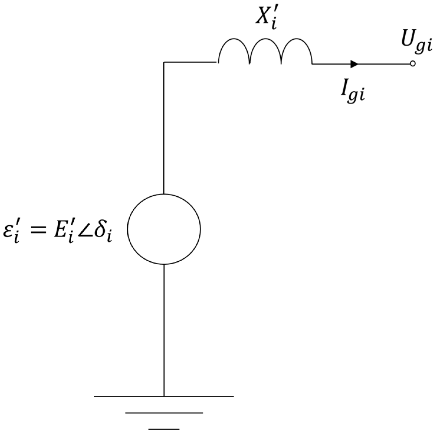
Modeling a multi-machine power system requires the representation of the generators, the electric network and the loads. Generators are represented with the classical model [21], which is summarized in Figure 1. In this model, each generator i is represented by an internal generator bus with voltage ${\epsilon }_i^{\prime }$ that has a constant magnitude $E_i^{\prime }$ and a varying phase angle ${\delta }_i$. A transient reactance $X_i^{\prime }$ connects the internal bus of generator i, which delivers the output phasor current $I_{gi}$, to the terminal bus of the generator with terminal voltage $U_{gi}$. Furthermore, the mechanical power input to each machine remains constant so that effects stemming from governor or excitation systems are neglected. Moreover, the mechanical rotor angle of a generator is assumed to coincide with the phase angle ${\delta }_i$ of the internal generator voltage ${\epsilon }_i^{\prime }$.

Figure 1. Classical generator model.

The dynamics of the phase angle ${\delta }_i$ and frequency ${\omega }_i$ of generator i are modeled by the swing equation:

$$\frac{d{\delta }_i}{dt}={\omega }_i-{\omega }_0$$

(7)

$$\frac{d{\omega }_i}{dt}=\frac{{\omega }_0}{2H_i}\left[P_{mi}-P_{ei}-\frac{D_i}{{\omega }_0}({\omega }_i-{\omega }_0)\right]$$

(8)

$$P_{ei}=\Re \left\{{\epsilon }_i^{\prime }{I}_{gi}^{*}\right\}$$

(9)

$$I_{gi}=\frac{{\epsilon }_i^{\prime }-U_{gi}}{j{X}_i^{\prime }}$$

(10)

where $P_{ei}$ is the electric power output, $P_{mi}$ is the mechanical power input, ${\omega }_0$ is the synchronous frequency, $H_i$ is the inertia constant and $D_i$ the damping constant.

The N-bus electric network is represented by the admittance matrix Y:

$$Y_{ij}=\{\begin{array}{c}{y}_{ii}+{\displaystyle {\displaystyle \sum }_{k=1, k\ne i}^N}{y}_{ik} if j=i\\ -y_{ij} if j\ne i\end{array}$$

(11)

where $y_{ik}$ is the summed admittance of all transmission lines connecting bus i and k possibly being zero if there is no connection between bus i and k and $y_{ii}$ is the shunt admittance at bus i. The current injections at generation buses $I_g$ as well as those at load buses $I_l$ can then be computed from the admittance matrix and the voltages at generation buses $U_g$ and those at load buses $U_l$:

$$\left[\begin{array}{cc}{Y}_{gg}& Y_{gl}\\ Y_{lg}& Y_{ll}\end{array}\right]\left[\begin{array}{c}{U}_g\\ U_l\end{array}\right]=\left[\begin{array}{c}{I}_g\\ I_l\end{array}\right]$$

(12)

If the electric network is expanded through the introduction of an internal generator bus for each generator, which is connected to its generation bus via a transient reactance as illustrated in Figure 1, and loads are modeled as constant impedances, the expanded network can be represented as:

$$\left[\begin{array}{ccc}{Y}^{\prime }& -Y^{\prime }& 0\\ -Y^{\prime }& Y^{\prime }+Y_{gg}& Y_{gl}\\ 0& Y_{\lg }& Y_{ll}+Y_l\end{array}\right]\left[\begin{array}{c}{\epsilon }^{\prime }\\ U_g\\ U_l\end{array}\right]=\left[\begin{array}{c}{I}_g\\ 0\\ 0\end{array}\right]$$

(13)

where the connection of the internal generator buses to the electric network is represented by:

$$Y^{\prime }=diag\left\{\frac{1}{j{X}_i^{\prime }}\right\}$$

(14)

and the loads are converted to constant admittances:

$$Y_l=diag\left\{\frac{P_{li}-j{Q}_{li}}{U_{li}^2}\right\}$$

(15)

where $P_{li}$ is the active and $Q_{li}$ the reactive load at bus i. Equation ($13$) is written as:

$$\left[\begin{array}{cc}{Y}_{11}& Y_{12}\\ Y_{21}& Y_{22}\end{array}\right]\left[\begin{array}{c}{\epsilon }^{\prime }\\ U_g\\ U_l\end{array}\right]=\left[\begin{array}{c}{I}_g\\ 0\\ 0\end{array}\right]$$

(16)

and the application of Kron’s reduction to Equation ($16$) yields the reduced representation of the network with all the buses except for the internal generator buses eliminated:

$$(Y_{11}-Y_{12}{Y}_{22}^{-1}{Y}_{21}){\epsilon }^{\prime }=Y_R{\epsilon }^{\prime }=I_g$$

(17)

where $Y_R$ is the reduced bus admittance matrix:

$$Y_R=G_R+j{B}_R$$

(18)

The active electric power output can then be formulated as a function of the internal generator voltages and the reduced admittance matrix:

$$P_{ei}=\Re \left\{{\epsilon }_i^{\prime }{I}_{gi}^{*}\right\}=\Re \left\{{\epsilon }_i^{\prime }{\displaystyle \sum }_{j=1}^{N_g}{Y}_{Rij}^{*}{\left({\epsilon }_j^{\prime }\right)}^{*}\right\}$$

(19)

where $N_g$ stands for the number of generators. Equation ($19$) can be reformulated to illustrate the nonlinear dependence of the electric power output on the generator phase angles:

$$P_{ei}={(E_i^{\prime })}^2{G}_{Rii}+{\displaystyle \sum }_{\begin{array}{c}j=1\\ j\ne i\end{array}}^{N_g}{E}_i^{\prime }{E}_j^{\prime }[G_{Rij}\cos \left({\delta }_i-{\delta }_j\right)+B_{Rij}\sin \left({\delta }_i-{\delta }_j\right)]$$

(20)

where $E_i^{\prime }$ is the constant magnitude of the internal machine voltage ${\epsilon }_i^{\prime }$, $G_{Rij}$ is the real and $B_{Rij}$ the imaginary part of the reduced admittance matrix according to Equation ($18$).

The transient simulation is initialized with a steady state load flow solution satisfying Equation (16), in which there is a match between mechanical power input and the electrical power output for every generator. A three-phase fault is then applied by modifying the admittance matrix of the system. The fault is assumed to occur close to a specific bus i so that the fault can be modeled by a fault shunt admittance of $y_{ii,fault}=-j{10}^9$. As a consequence of the fault, the balance between the mechanical power input and electrical power output of the generators is lost causing the rotor angles and frequencies to deviate from their initial values. The dynamics of this process is modeled by Equations ($7$) and ($8$) directly affecting the electric power outputs of the generators according to Equation ($20$).

The three-phase fault is cleared after a certain time by opening the faulted line. Thus, the admittance matrix is modified for the post-fault period by removing the fault admittance $y_{ii,fault}$ and the new topology without the opened line forms the post-fault admittance matrix. Depending on the fault clearing time, some of the generators may increase their kinetic energy and enter uncontrolled spinning.

Transient stability of a power system refers to the ability of its synchronous generators to remain in synchronism after a severe disturbance. It can be assessed by computing all generator phase angles as a function of time by numerical integration of Equations ($7$) and ($8$). Generators are in synchronism if all phase angle differences among generators remain bounded. If the increase in phase angle difference between a specific generator and the remaining generators is unbounded, that generator is said to lose synchronism or to go out-of-step with the remaining generators.

4. Grid Splitting

Generally, a loss of synchronism due to severe disturbances in a power system causes large variations in power flows and voltages. These variations may trigger relay operations at different network locations, which can further aggravate the disturbance and possibly lead to cascading outages and power blackouts [22]. Under the condition of an impending instability in the initial network, grid splitting aims at changing the topology of the electric network through the disconnection of certain transmission lines. This action is implemented in the model by the adjustment of the admittance matrix to the new topology. The aim of grid splitting is to create islands that group generators, which are expected to remain synchronous.

In this study, the SCCI algorithm [17] is applied as an offline procedure to identify suitable clusters of the initial network for the following island formation. This islanding solution is found by using spectral clustering which groups the buses into clusters which cause the minimum power flow disruption after grid splitting, while satisfying the constraint of coherent generator groups. The SCCI algorithm works in two steps, namely, (i) the generator buses which host generators that remain synchronous are divided into coherent groups, (ii) the remaining buses, i.e., purely load buses, are assigned to coherent generator groups.

In order to find coherent generator groups, the dynamic coupling S between two disjoint generator subsets $V_{G1}$ and $V_{G2}$ of $V_G$, a set that contains all buses with generators connected to them, needs to be analyzed. The dynamic coupling S can be calculated using the theory of slow coherency:

$$S={\displaystyle \sum }_{j\in V_{G2}}{\displaystyle \sum }_{i\in V_{G1}}\left(\frac{\partial P_{ij}}{\partial {\delta }_{ij}}\times \left(\frac{1}{H_i}+\frac{1}{H_j}\right)\right)$$

(21)

where generator i belongs to subset $V_{G1}$, generator j belongs to subset $V_{G2}$, and $\frac{\partial P_{ij}}{\partial {\delta }_{ij}}$ is the synchronizing coefficient between generator i and j.

Generators with a strong dynamic coupling will swing together and generators with weak dynamic coupling will swing against each other when exposed to electromechanical oscillations [23]. The identification of coherent generator groups can mathematically be formulated as an optimization problem that finds the weakest dynamic coupling between generator groups:

$$\left[V_{G1}^{*},V_{G2}^{*}\right]=\underset{V_{G1},V_{G2}\subset V_G}{\min }(S)$$

(22)

where $V_{G1}^{*}$ and $V_{G2}^{*}$ are the resulting subsets of $V_G$ in case of a bisection. The identified coherent generator groups serve as a constraint of the optimization problem that identifies the two disjoint subsets $V_1$ and $V_2$ of V, a set that includes all buses of the network:

$$\underset{\begin{array}{c}{V}_1,V_2\subset V\\ subject to V_{G1}^{*}\subset V_1 V_{G2}^{*}\subset V_2 \end{array}}{\min }\left({\displaystyle \sum }_{i\in V_1, j\in V_2}\left|P_{ij}\right|\right)$$

(23)

The objective function used in Equation ($23$) is the sum of the active power of the transmission lines that are disconnected in the grid-splitting procedure. Thus, the optimization problem described by Equation ($23$) finds islands that minimize the power flow disruption so that the change from the pre-disturbance power flow pattern due to the grid-splitting action is minimized. As a consequence, transient stability in the created islands is improved, the possibility of transmission line overloads within the island is reduced, and the eventual reintegration of the islands with the rest of the system is eased [24].

The optimization problems in Equations ($22$) and ($23$) are converted into graph-cut problems and solved using spectral clustering. The application of recursive bisection allows the system to be split in more than two islands.

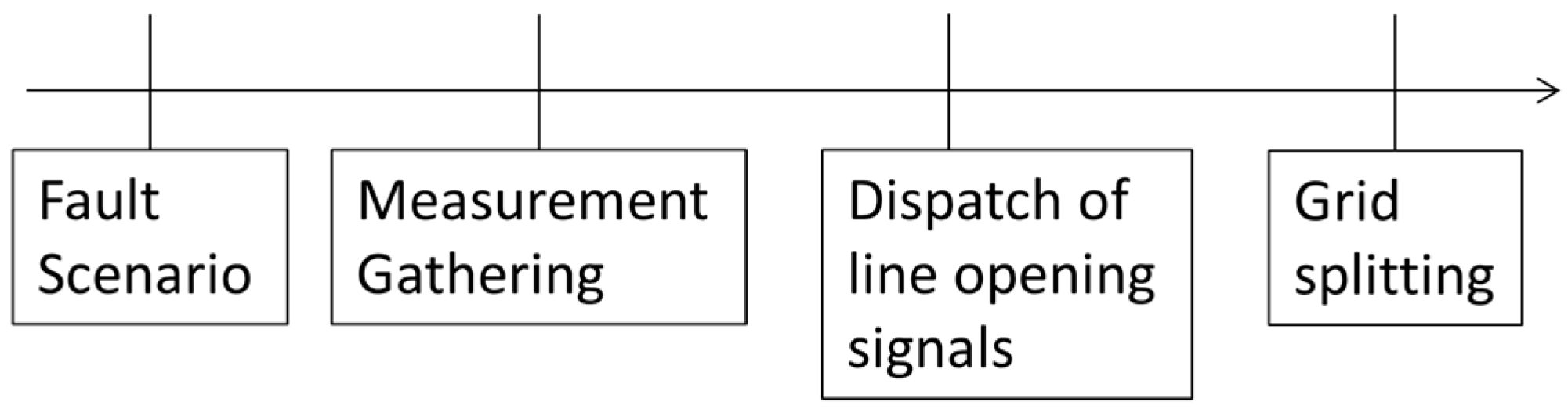
After identifying the splitting locations, grid splitting is executed, which involves the transmission of several signals over the communication network:

• Each bus j dispatches a synchrophasor measurement to the control center with a time delay $T_{bus,j}$ directly after fault clearing.
• The line opening signal for line i is dispatched with a delay $T_{open,i}$ from the control center to the appropriate bus once the instability is detected. If it is detected after receiving all synchrophasor measurements, each line opening signal will be dispatched directly after the arrival of the last synchrophasor measurement.

A timeline of events that happen during the grid-splitting procedure is provided in Figure 2.

Figure 2. Timeline of events for the grid-splitting procedure.

The time delay $T_i$ of line i from the clearing of the fault until its disconnection is then given by

$$T_i=\underset{1\le j\le N}{\max }{T}_{bus,j}+T_{open,i}$$

(24)

for an N-bus electric network under the assumption that there are no delays due to discretization or processing of data.

As a result of grid splitting, some islands might still be unstable, and therefore the stabilization attempt is unsuccessful. The performance of grid splitting is evaluated based on the amount of load that can be supplied to the customers after grid splitting. Under the assumption that the entire load in an unstable island is lost, the demand served DS [25] can be computed as

$$DS=\frac{{{\displaystyle \sum }}_{i=1, i\ne j}^M{P}_{l,i}}{{{\displaystyle \sum }}_{i=1}^M{P}_{l,i}}$$

(25)

where $P_{l,i}$ is the active load in island i, M is the total number of islands and islands j consist of all unstable islands. The application of the proposed metric can be exemplified with reference to the 2003 blackout in southern Sweden and eastern Denmark [26,27]. Prior to that disturbance, the demand was around 15,000 MW in Sweden and 1850 MW in eastern Denmark, leading to a total pre-disturbance load of 16,850 MW. The load lost due to the disturbance was approximately 4500 MW in Sweden and 1850 MW in eastern Denmark. Thus, the demand served following the event was DS = 0.377.

5. Case Study

In this study, the IEEE 39-Bus System and the IEEE 118-Bus System are investigated. These electric systems are coupled with a dedicated communication network. For simplicity but with no loss of generality, the communication network consists of dedicated control signal channels connecting the routers, which follow the same layout as the electrical transmission lines connecting the buses. The physical lengths of the communication channels are estimated based on the transmission line reactance [28].

The transient simulation is initialized with a pre-fault load flow solution using the optimal power flow (OPF) solver of MATPOWER [29]. The optimization is based on the minimization of generation costs subject to bus voltage, generation and branch flow constraints. In order to represent variability in the system-loading conditions, a load factor, LF, is introduced that scales the active and the reactive power at each bus.

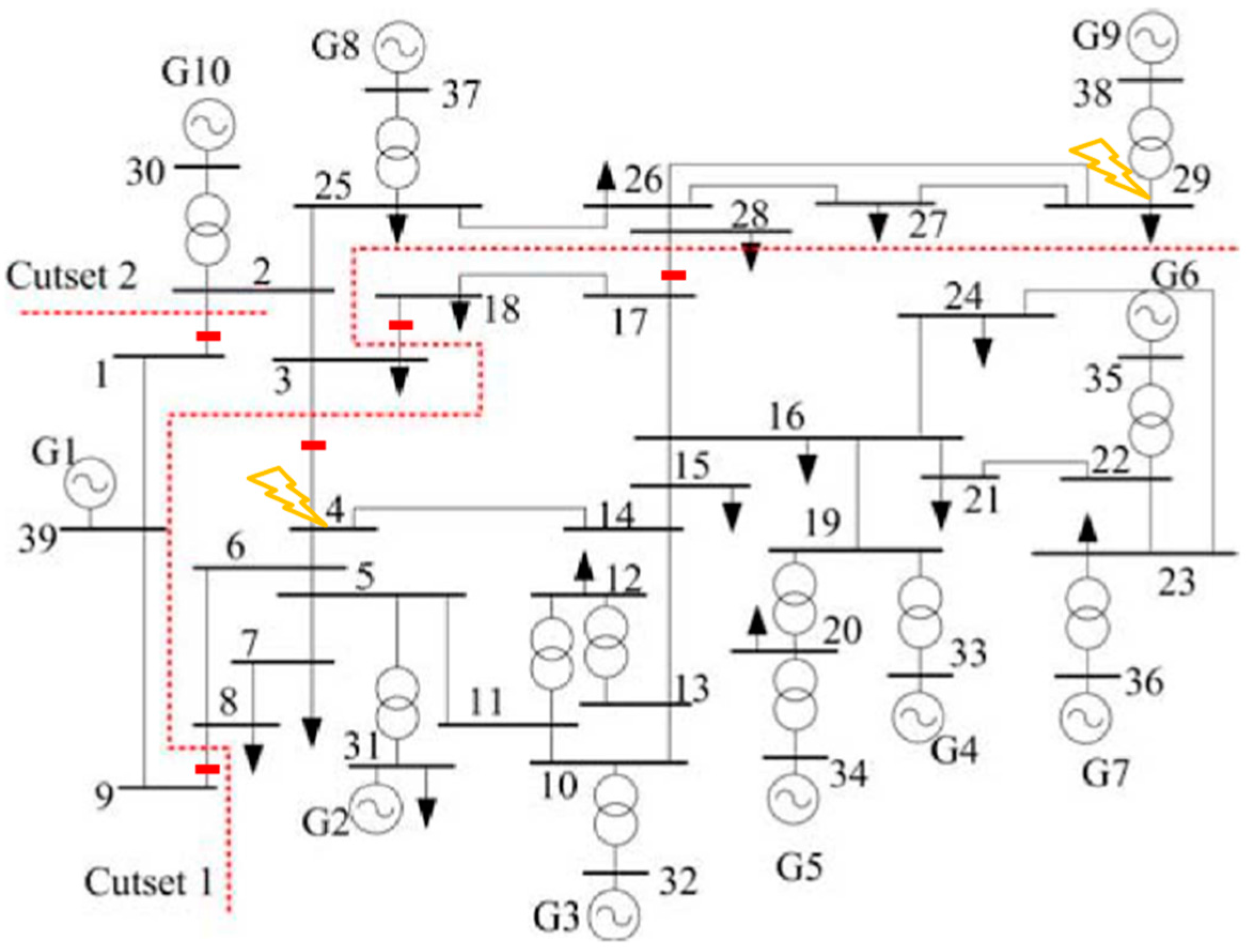
5.1. IEEE 39-Bus System

Figure 3 shows the schematic of the IEEE 39-Bus Test System. The five splitting locations are indicated by thick bars and the resulting three clusters are identified by dashed lines. The parameters of the communication network as well as the assessed load factors are reported in Table 1. In particular, all communication links work at the same data rate $D_r$, and the same router serving rate μ is associated with the routing delays experienced at the communication nodes.

Figure 3. Single-line diagram of the IEEE 39-Bus Test System. The dotted lines represent the two cut sets necessary to produce the final islanding solution via grid splitting [17]. The disconnected lines indicated by bars are line 1–2, 3–4, 8–9, 17–28, 3–18. The contingencies are applied at Bus 4 and 29. The control center is located at Bus 13.

Table 1. Specifications of the electric power grid and of the communication network used in the simulations.

Data Rate	$D_r$	$5\times {10}^4-2\times {10}^5$bit/s
Packet size	$P_s$	$2$Kbit
Between packet delay	$T_b$	$0$ s
Data velocity	$v$	$0.6$ c
Measurement rate	$\lambda$	$50$packets/s
Router serving rate	$\mu$	$5$ Mbit/s
Load factor	$LF$	0.9–1.09

The contingency is generated by applying a three-phase fault on a line located in the proximity of bus 29 at $t=1 \mathrm{s}$. The contingency is cleared at $t=1.2 \mathrm{s}$ by opening, i.e., disconnecting, line 28–29, i.e., line connecting bus 28 and bus 29. A second fault is then applied on a line located in the proximity of bus 4 at $t=1.3 \mathrm{s}$ and cleared at $t=1.9 \mathrm{s}$ by opening line 4–5. These faults result in a loss of synchronism among generators, if no mitigation action takes place, which is demonstrated in this case study.

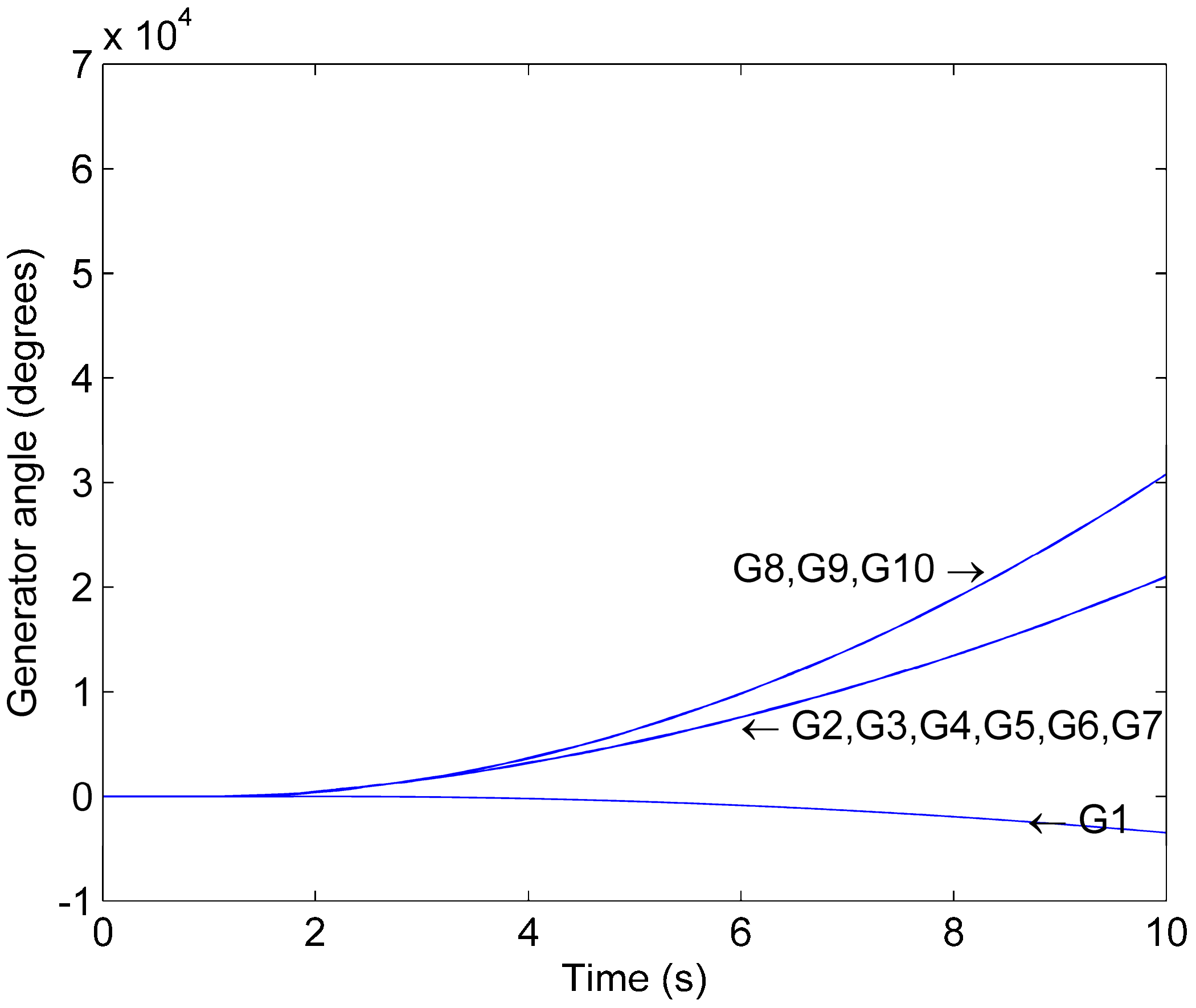
To show the effects of both the load conditions and the data rate of the communication network on the successful application of grid splitting as a mitigation action, four scenarios are presented. The chosen parameters for each scenario are given in Table 2. Scenario 1 represents a situation without grid splitting and communication. In Scenario 2, communication and grid splitting are introduced. Scenario 3 represents a configuration with degraded communication compared to Scenario 2. Stressful loading conditions are represented by Scenario 4.

Table 2. Simulation parameters used for the different scenarios.

Scenario	${\mathit{D}}_{\mathit{r}}$ (bit/s)	$\mathit{L}\mathit{F}$ (-)
1	No communication	0.95
2	$2\times {10}^5$	0.95
3	$5\times {10}^4$	0.95
4	$2\times {10}^5$	1.05

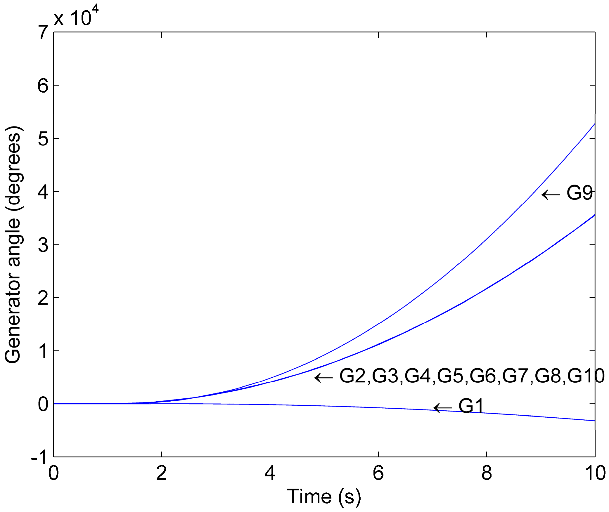
Figure 4 shows the generator phase angles as a function of time for Scenario 1. Generator 1 and 9 lose synchronism with respect to the other generators following the initial contingency. Therefore, there is a loss of synchronism among generators if no mitigation action is applied after the initial contingency occurs. System studies show that the loss of synchronism following the fault contingency occurs for all the investigated loading conditions.

Figure 4. Phase angle trajectory for Scenario 1.

Scenario 2 demonstrates that if a splitting action, which is supported by a high data-rate communication network, is carried out after the contingency, the system can be stabilized. In Scenario 2, the communication network transmits synchrophasor measurement signals from all bus locations to the control center situated at the central location of bus 13 directly after clearing the second fault. Then, line opening signals are dispatched from the control center to the splitting locations upon reception of the last synchrophasor measurement. The splitting locations are identified offline using the SCCI algorithm [17] and are independent of the fault scenario. The delay to disconnect the affected lines is calculated according to Equation ($24$). As a result, the network is split into three islands. The allocation of the ten generators to the three islands is reported in Table 3.

Table 3. Allocation of the generators to the islands.

Island	Generators
1	G2, G3, G4, G5, G6, G7
2	G8, G9, G10
3	G1

Figure 5 shows the generator phase angles as a function of time for Scenario 2. Since the phase angles of all generators that belong to the same island coincide it can be concluded that grid splitting successfully stabilizes the three islands.

Figure 5. Phase angle trajectory for Scenario 2.

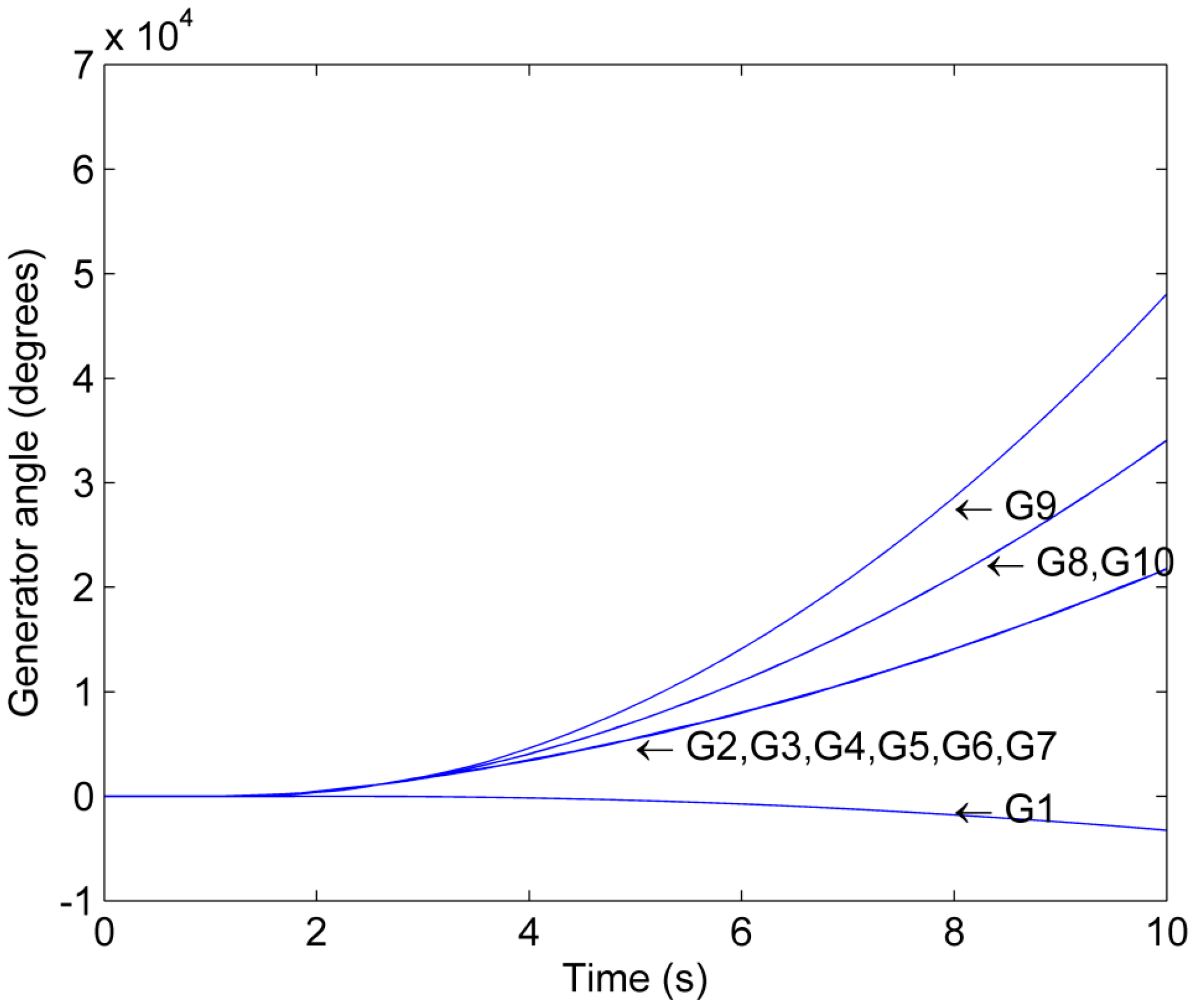
A comparison of Scenario 2 and Scenario 3 illustrates the impact of the communication network parameters on the application of grid splitting. In Scenario 3, the data rate $D_r$ of the communication network is reduced by one order of magnitude as compared to Scenario 2 (Table 2). This leads to an increase of the delays in the transmission of information across the communication network. Figure 6 shows the generator phase angles as a function of time for Scenario 3. As opposed to Scenario 2, the splitting action cannot prevent Generator 9 from separating from Generator 8 and 10 so that Island 2 becomes unstable. Therefore, the success of the splitting action in mitigating the incumbent system instability is dependent on its timely execution. This finding is consistent with observations made in the literature reporting that the splitting will become unsuccessful if an acceptable maximal splitting delay period (ASDP) following the fault scenario is exceeded [30].

Figure 6. Phase angle trajectory for Scenario 3.

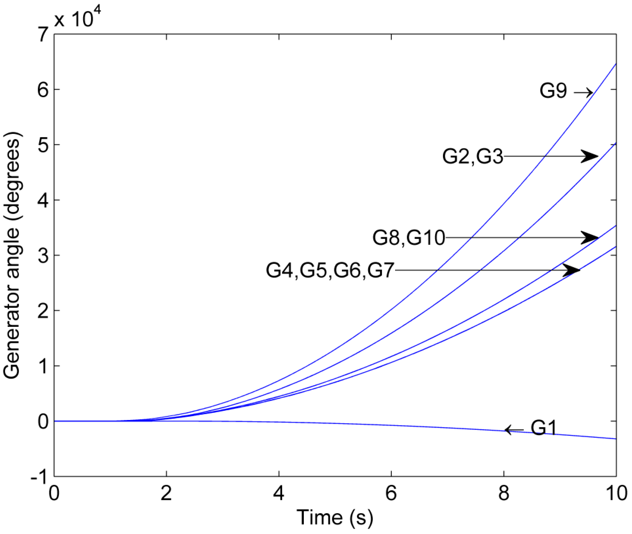
A comparison of Scenario 4 and Scenario 2 illustrates that the outcome of the grid splitting is dependent on the loading conditions of the network. Figure 7 shows the generator phase angles as a function of time for Scenario 4. It can be observed that both Island 1 and 2 become unstable despite the stabilization attempt through grid splitting. In Island 1, Generator 2 and 3 separate from the remaining generators in the island, whereas in Island 3, Generator 9 separates from Generator 8 and 10. The stabilization attempt is unsuccessful because the increase in LF from 0.95 in Scenario 2 to 1.05 in Scenario 4 has pushed the power system closer to its stability limit [31].

Figure 7. Phase angle trajectory for Scenario 4.

In summary, Scenario 1 illustrates that there is a loss of synchronism among generators following the faults if no mitigation action takes place. Scenario 2 shows that the system can be stabilized and, thus, all generators remain in synchronism by splitting the grid into three islands. However, Scenario 3 shows that the outcome of the stabilization attempt by grid splitting depends on the parameters of the communication infrastructure and that it will be unsuccessful if communication is degraded. Furthermore, Scenario 4 demonstrates that an increase in the loading of the system can negatively affect the outcome of grid splitting.

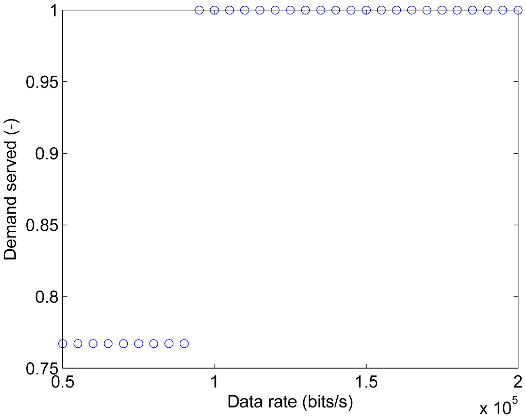
In order to characterize the impact of degraded communication and varying loading conditions on grid splitting, the effects of increasing time delays and load conditions on the performance of the grid-splitting action are quantified. Figure 8 presents the demand served of grid splitting defined according to Equation ($25$) for a constant load factor $LF=0.95$ and a varying data rate of the communication network. Demand served equal to 0.767 is achieved for data rates between $5\times {10}^4$ and $9\times {10}^4$bit/s and it corresponds to instability in Island 2 and stability in both Island 1 and 3. A stabilization of all three islands can be achieved with data rates between $9.5\times {10}^4$ and $2\times {10}^5$ bit/s corresponding to a demand served equal to 1.

Figure 8. Demand served of grid splitting as a function of the data rate for a constant load factor $\text{LF}=0.95$.

For real systems, different data rates are reported in the literature. In [15], a data rate of $6.4\times {10}^4$ bit/s is reported, which does not meet the required critical data rate $D_r^{*}=9.5\times {10}^4$ bit/s. In [32], a data rate of $2\times {10}^6$ bit/s is used corresponding to a margin of $1.905\times {10}^6$ bit/s.

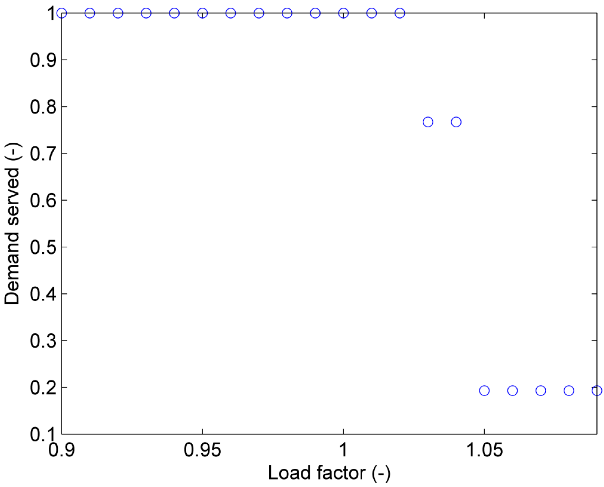
Figure 9 shows the results of the demand served of the grid-splitting action for a fixed data rate of $2\times {10}^5$ bit/s and load factors varying between 0.9 and 1.09. Load factors between 0.9 and 1.02 yield a demand served of 1, meaning that the chosen data rate is sufficient to stabilize all three islands. An increase of the load factor to 1.03 leads to a decrease in the demand served to 0.767 corresponding to a loss of synchronism in Island 2 after grid spitting. If the load factor is further increased to 1.05, Island 1 is also destabilized, further reducing the demand served to 0.193.

Figure 9. Demand served of grid splitting as a function of the load factor LF for a constant data rate $D_r=2\times {10}^5$ bit/s.

5.2. IEEE 118-Bus System

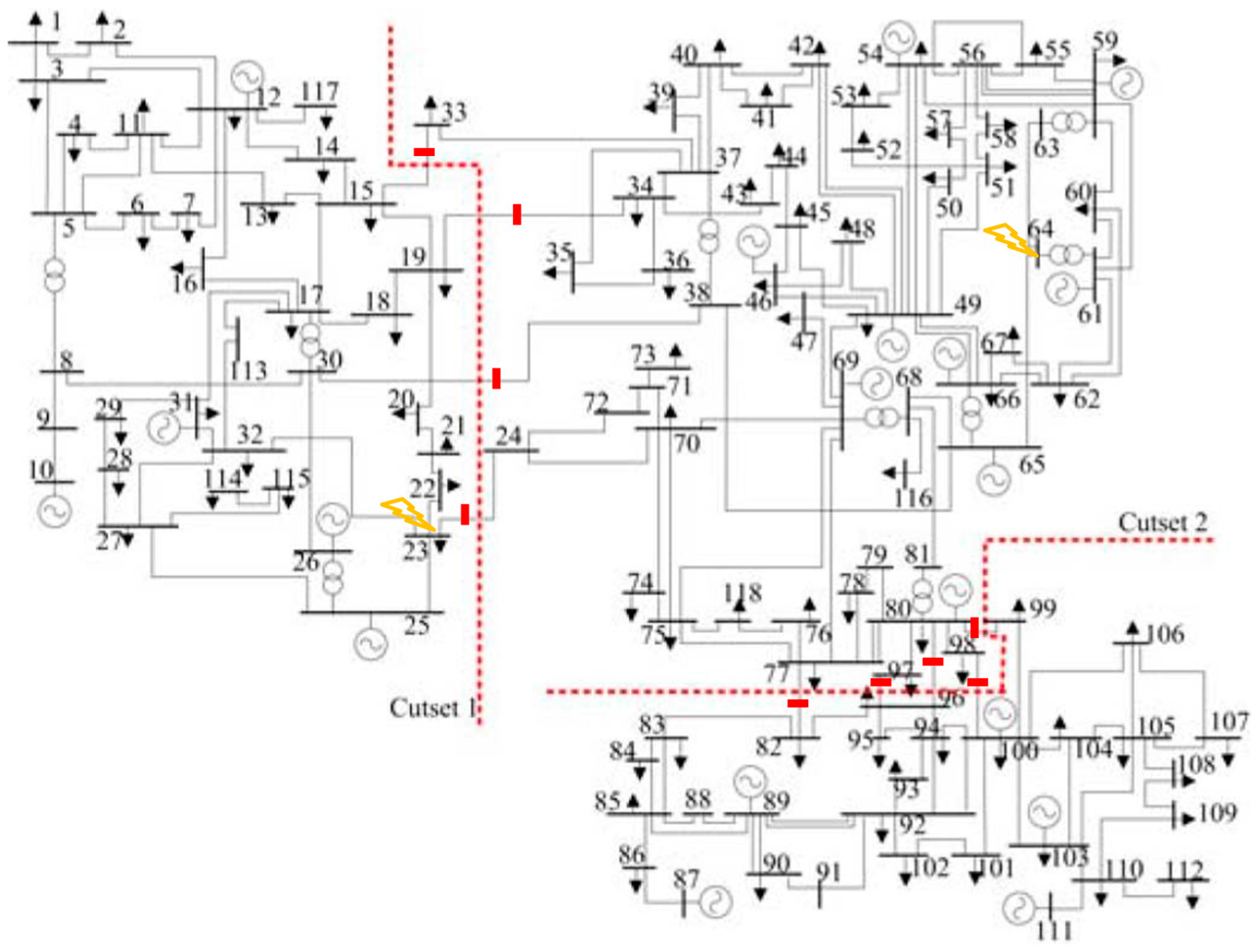
Figure 10 shows the schematic of the IEEE 118-Bus Test System. The nine splitting locations are indicated by thick bars and the resulting three clusters are identified by dashed lines. The parameters of the generators are taken from [30], and those of the communication network as well as the assessed load factors are reported in Table 4.

Figure 10. Single-line diagram of the IEEE 118-Bus Test System. The dotted lines represent the two cut sets necessary to produce the final islanding solution via grid splitting [17]. The disconnected lines indicated by bars are line 15–33, 19–34, 30–38, 23–24, 77–82, 96–97, 80–96, 98–100, 80–99. The contingencies are applied at Bus 23 and 64. The control center is located at Bus 73.

Table 4. Specifications of the electric power grid and of the communication network used in the simulations.

Data Rate	$D_r$	$7\times {10}^4-7\times {10}^5$bit/s
Packet size	$P_s$	$2$Kbit
Between packet delay	$T_b$	$0$ s
Data velocity	$v$	$0.6$ c
Measurement rate	$\lambda$	$50$packets/s
Router serving rate	$\mu$	$5$ Mbit/s
Load factor	$LF$	0.9–1.25

The contingency is generated by applying a three-phase fault on a line located in the proximity of bus 64 at $t=1 \mathrm{s}$. The contingency is cleared at $t=1.4$s by opening line 64–65. A second fault is then applied on a line located in the proximity of bus 23 at $t=1.5 s$ and cleared at $t=1.95 s$ by opening line 22–23. These faults result in a loss of synchronism among generators, if no mitigation action takes place, which is demonstrated in this case study.

As in the 39-Bus System case study, four scenarios are presented to show the effects of both the load conditions and the data rate of the communication network on the successful application of grid splitting as a mitigation action. Table 5 summarizes the parameters for each scenario.

Table 5. Simulation parameters used for the different scenarios.

Scenario	${\mathit{D}}_{\mathit{r}}$ (bit/s)	$\mathit{L}\mathit{F}$ (-)
1	No communication	0.90
2	$5\times {10}^5$	0.90
3	$7\times {10}^4$	0.90
4	$5\times {10}^5$	1.05

Scenario 1 represents a situation without grid splitting and communication. In Scenario 2, communication and grid splitting are introduced. Scenario 3 represents a configuration with degraded communication compared to Scenario 2. Stressful loading conditions are represented by Scenario 4.

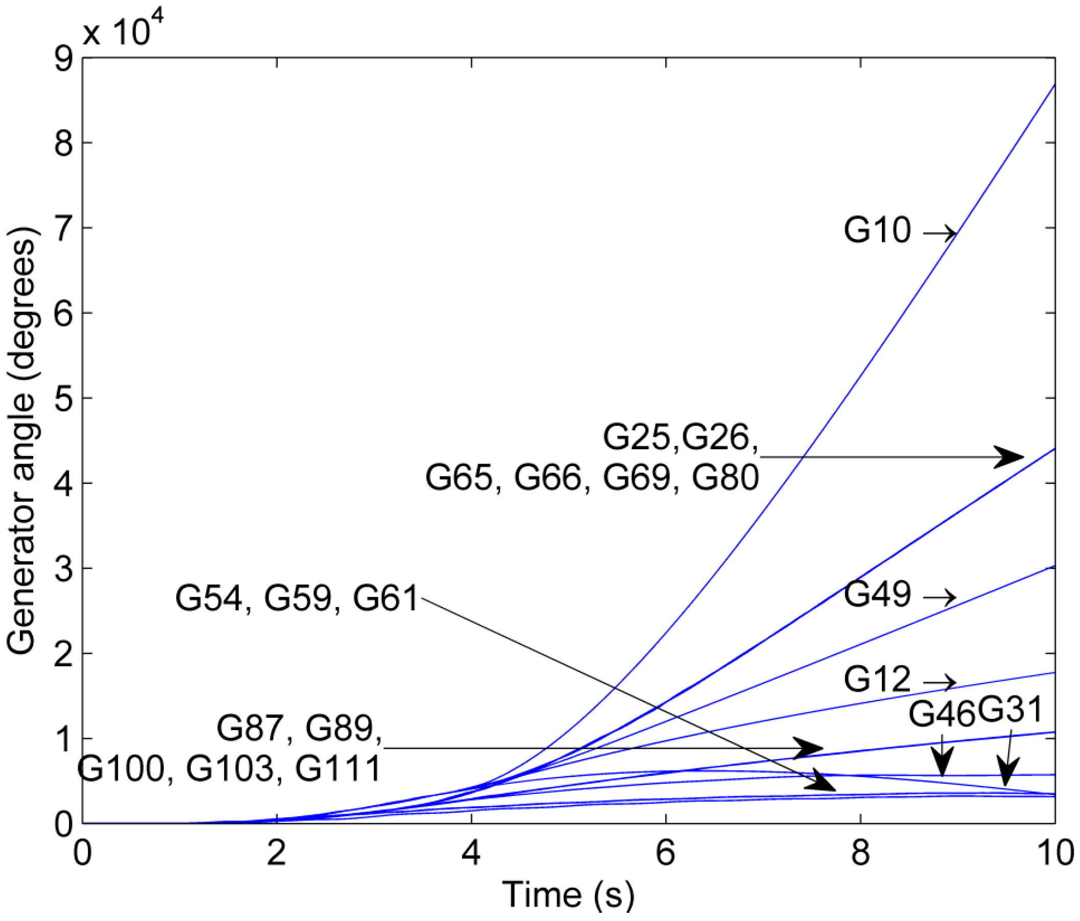
Figure 11 shows the generator phase angles as a function of time for Scenario 1. A loss of synchronism following the initial contingency can be observed since the phase angle differences among generators do not remain bounded. System studies show that this loss of synchronism occurs for all the investigated loading conditions if no mitigation action takes place.

Figure 11. Phase angle trajectory for Scenario 1.

In Scenario 2, a successful stabilization through a splitting action supported by a high data-rate communication network is demonstrated, similar to Scenario 2 of the 39-Bus System case study. As a result, the network is split into three islands using the SCCI algorithm [17]. The allocation of the 19 generators to the three islands is reported in Table 6.

Table 6. Allocation of the generators to the islands.

Island	Generators
1	G10, G12, G25, G26, G31
2	G46, G49, G54, G59, G61, G65, G66, G69, G80
3	G87, G89, G100, G103, G111

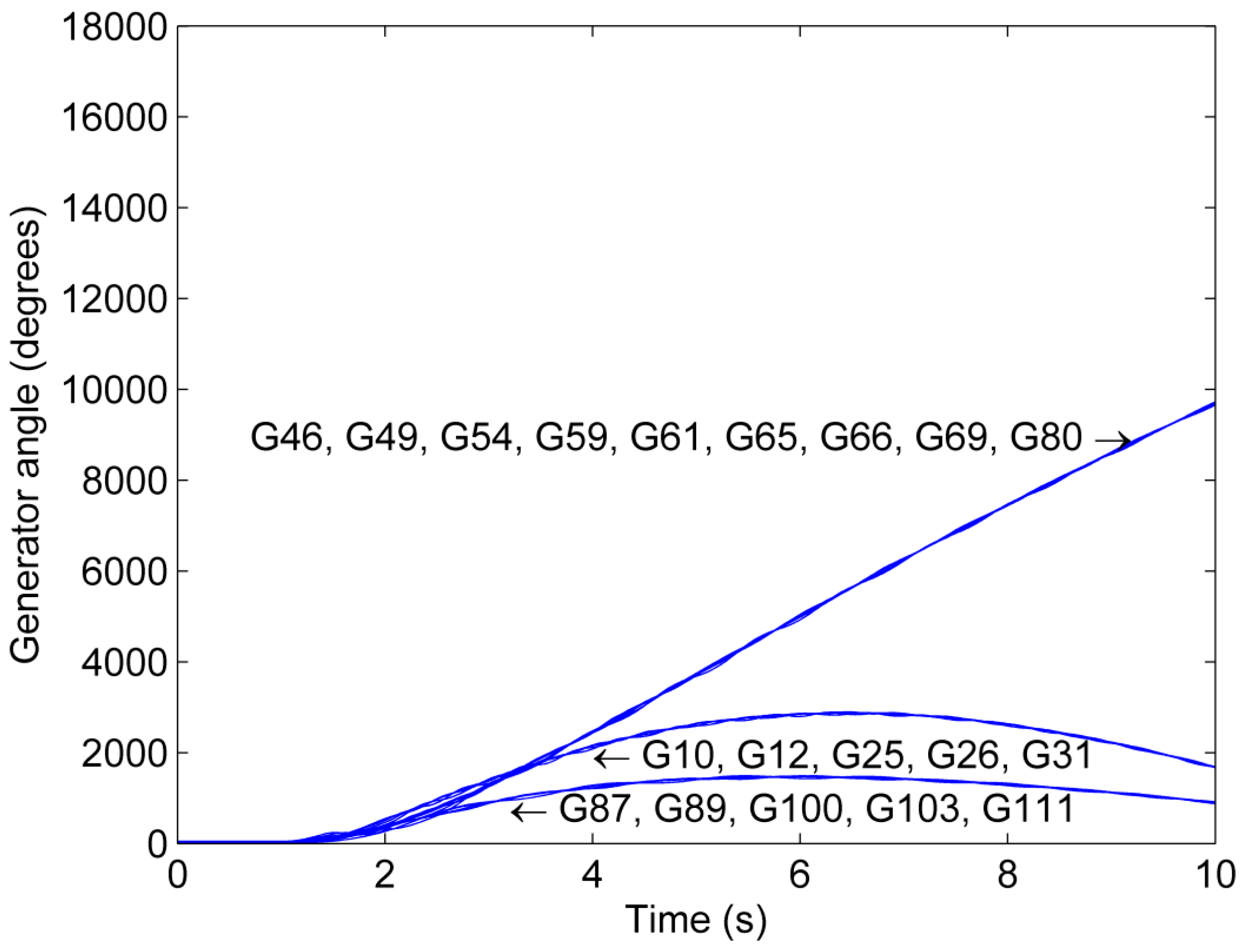
Figure 12 shows the generator phase angles as a function of time for Scenario 2. The grid-splitting action successfully stabilizes all three islands because the phase angles of all generators belonging to the same island coincide.

Figure 12. Phase angle trajectory for Scenario 2.

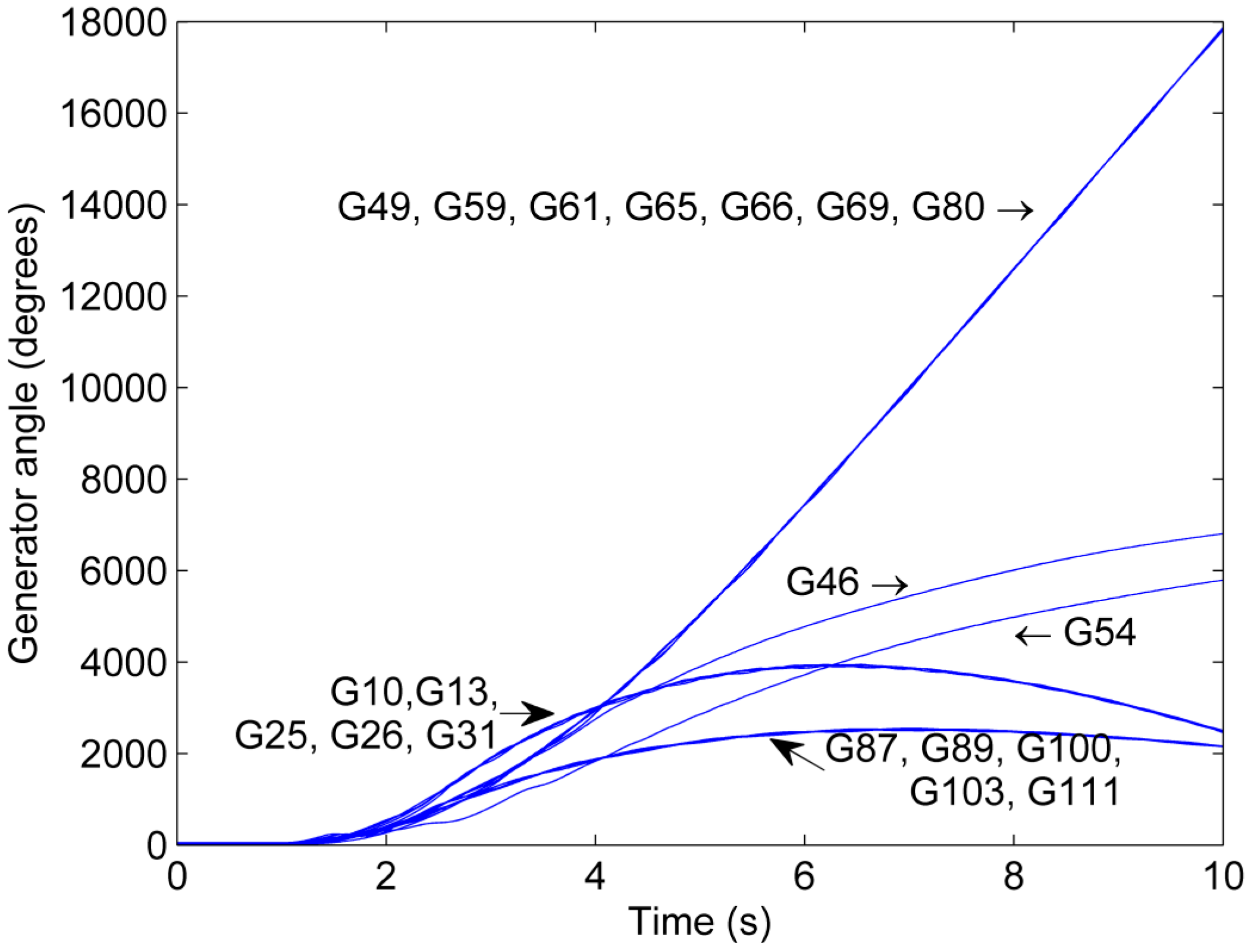
In Scenario 3, the data rate $D_r$ of the communication network is reduced by one order of magnitude as compared to Scenario 2 (Table 5). This leads to an increase of the delays in the transmission of information across the communication network. Figure 13 shows the generator phase angles as a function of time for Scenario 3. It can be observed that the reduction of the data rate $D_r$ leads to a loss of synchronism in Island 2 since Generator 46 and 54 separate from the remaining generators in Island 2. Thus, the reduction of the data rate in Scenario 3 compared to Scenario 2 causes the stabilization attempt to become unsuccessful because the acceptable maximal splitting delay period (ASDP) [30] is exceeded.

Figure 13. Phase angle trajectory for Scenario 3.

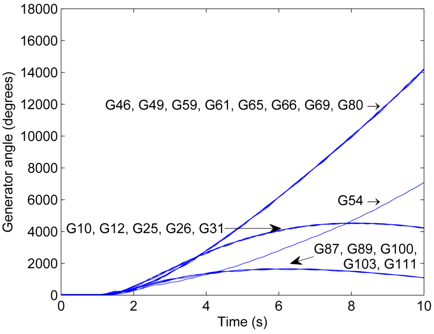
A comparison of Scenario 4 and 2 illustrates that the loading conditions affect the outcome of the grid splitting. The generator phase angles for Scenario 4 are shown in Figure 14. The stabilization attempt for Island 2 is unsuccessful because Generator 54 loses synchronism to the remaining generators. The outcome of the splitting attempt can be explained by an operation of the system closer to its stability limits in Scenario 4 as compared to Scenario 2 due to the increase in LF from 0.9 in Scenario 2 to 1.05 in Scenario 4 [31].

Figure 14. Phase angle trajectory for Scenario 4.

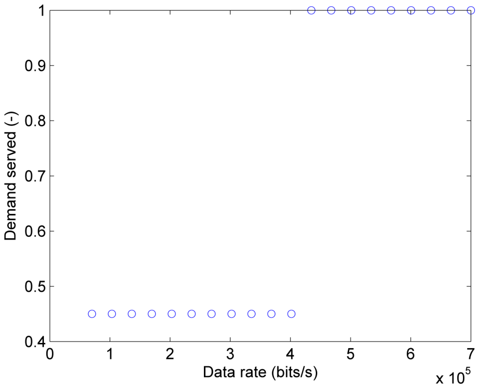
The effects of increasing time delays and load conditions on the successful application of grid splitting are quantified to characterize the impact of degraded communication and varying loading conditions. Figure 15 shows the demand served, DS, defined according to Equation ($25$) for a constant load factor $LF=0.9$ and a varying data rate $D_r$ of the communication network. Demand served equal to 0.45 is achieved for data rates between $7\times {10}^4$ bit/s and $4\times {10}^5$ bit/s and it corresponds to instability in Island 2 and stability in Island 1 and 3. All three islands can be stabilized with data rates between $4.3\times {10}^5$ bit/s and $7\times {10}^5$ bit/s corresponding to DS = 1.

Figure 15. Demand served of grid splitting as a function of the data rate for a constant load factor $LF=0.9$.

The critical data rate $D_r^{*}=4.3\times {10}^5$ bit/s exceeds the data rate of $6.4\times {10}^4$ bit/s for real systems reported in [15] and is below the data rate of $2\times {10}^6$ bit/s reported in [32], yielding a margin of $1.57\times {10}^6$ bit/s.

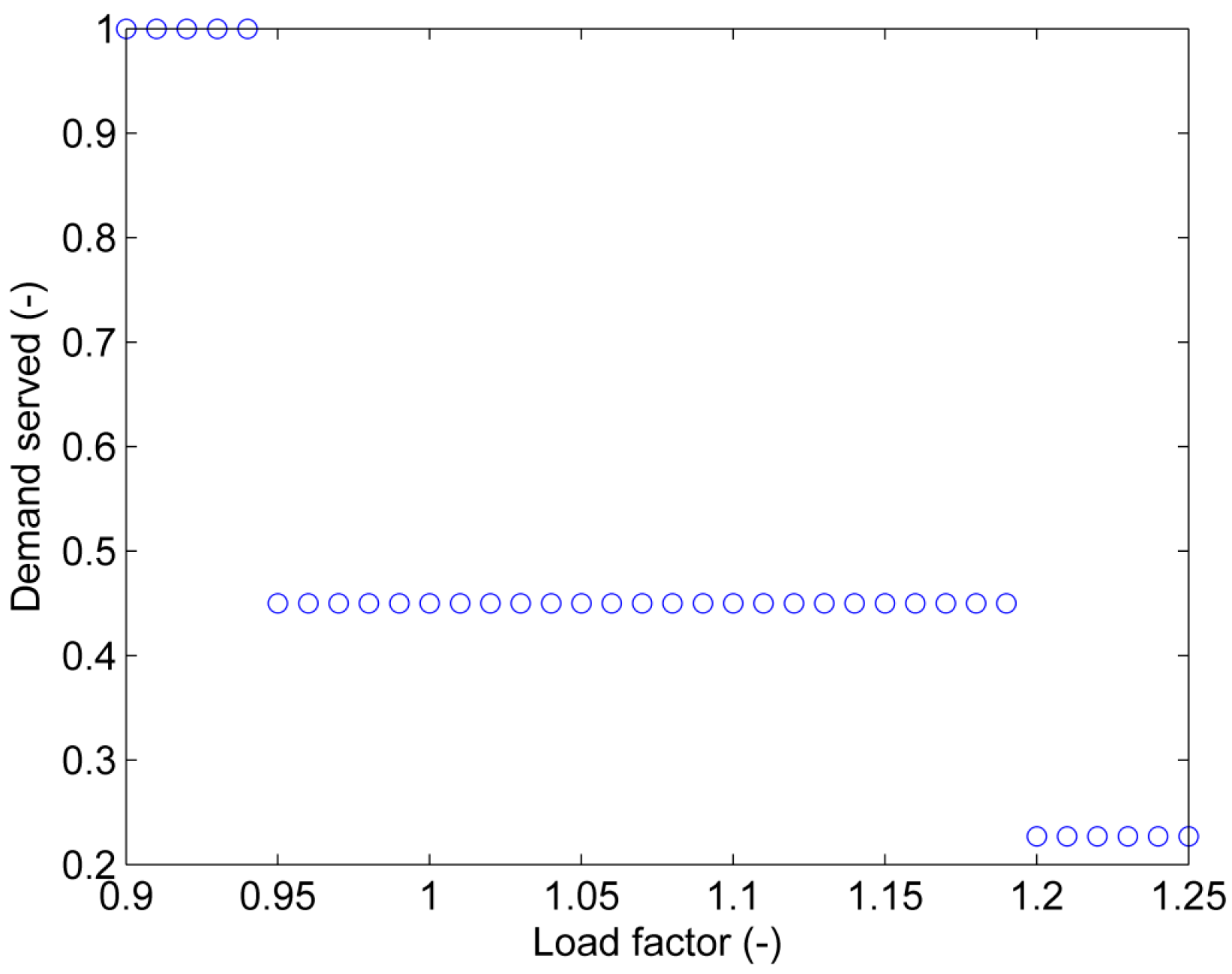
Figure 16 shows the results of the demand served DS of grid splitting for a fixed data rate of $5\times {10}^5$ bit/s and load factors between 0.9 and 1.25. Load factors between 0.9 and 0.94 yield a DS = 1 meaning that the chosen data rate is sufficient to stabilize all three islands. An increase of the load factor to 0.95 leads to a decrease in the demand served to 0.45 corresponding to a loss of synchronism in Island 2 after grid splitting. A further increase in the load factor to 1.2 causes the destabilization of Island 3, reducing the demand served to 0.227.

Figure 16. Demand served of grid splitting as a function of the load factor $LF$ for a constant data rate $D_r=5\times {10}^5$ bit/s.

6. Conclusions

In this study, the performance of grid splitting in power grids is studied as a topical application which highlights and entails strong interdependency among communications and electric power grids. To this aim, a communication delay model is coupled with a transient model of the electric system, which includes generators, an electric network and loads. Grid splitting requires a communication infrastructure to collect measurements for state estimation and to relay the command to open line switches. The application to the IEEE 39-Bus and the IEEE 118-Bus Test System shows that the loss of synchronism as a consequence of a fault scenario can be mitigated by splitting each system into three islands.

The results show that the success of the grid splitting strongly depends both on the parameters of the communication infrastructure to transmit measurement and line switch opening signals and on the loading conditions. An assessment of degraded communication in terms of the data rate of the communication network on the outcome of the grid splitting protection scheme for the IEEE 39-Bus System shows that for a load factor of 0.95, a data rate of $9.5\times {10}^4$ bit/s is sufficient to stabilize all three islands. For the IEEE 118-Bus System, a data rate of $4.3\times {10}^5$ bit/s is found to be sufficient to stabilize all three islands for a load factor of 0.9. The investigation of the influence of different loading conditions in the two systems shows that increased network flows can degrade the performance of grid splitting and cause some grid-splitting actions to become unsuccessful. Therefore, in general, it can be shown that large network flows and degraded communication have the potential to worsen the performance of grid splitting as a mitigating action.

The presented study introduces the assessment of the grid-splitting performance and exemplifies it with reference to two test systems with specific initial contingencies. These results can guide the thorough quantifications of grid-splitting performance for actual electric power infrastructures when the most severe contingencies and load conditions are assessed. Following this framework, a system-specific analysis can identify the requirements of the dedicated communication infrastructure for a successful grid-splitting procedure for a particular power system.