Safety-Constrained Energy-Efficient Control for High-Speed Trains Considering Wheel–Rail Interaction

Abstract

During train operation, the adhesion characteristics between the wheels and rails, which are influenced by driving environments and operating conditions, result in a traction force lower than the motor’s nominal output. Traditional control strategies often overlook the nonlinear relationship between wheel–rail adhesion limits and traction motor output, which can lead to wheel slippage, accelerated wear, and excessive energy consumption. This paper establishes an energy-efficient train control model considering wheel–rail adhesion characteristics. Based on convex optimization methods, the model jointly optimizes the train’s speed trajectory and motor control strategy. Before optimization, nonlinear constraints are simplified through function approximation and tightened McCormick envelope relaxation, significantly reducing the computational complexity of the model. Numerical experiments demonstrate that the proposed driving strategy can adjust the train’s speed in response to poor rail conditions, ensuring adherence to adhesion safety limits. Simulations based on real-world high-speed rail line data in China show that, compared to the traditional EETC model with anti-skid control measures, the proposed model achieves a safer driving strategy. Additionally, in the context of speed trajectory tracking control, it reduces energy consumption by 19.49% compared to the traditional EETC model with anti-skid control measures. Furthermore, the model demonstrates high computational efficiency, indicating its potential for integration into a real-time driving strategy optimization framework.

1. Introduction

The interaction between the wheels and rails of high-speed trains exhibits highly complex and nonlinear dynamic characteristics, making them susceptible to unsafe conditions like wheel slip or skidding, especially under adverse weather such as rain or snow. This not only results in a significant loss of energy due to the reduced motor power output but also causes irreparable damage to the rail surface, thereby shortening the lifespan of both the rails and wheels. In extreme cases, such issues may even lead to safety incidents. Therefore, it is crucial to incorporate the dynamic coupling behavior of the wheel–rail system when designing energy-efficient driving strategies.

Energy-Efficient Train Control (EETC), also referred to as eco-driving technology, has become a focal point of research in recent years. Current approaches to EETC can be generally categorized into indirect methods, direct methods, and intelligent optimization techniques [1]. Indirect methods, often grounded in optimal control theory, utilize the Pontryagin maximum principle to derive the optimal sequence for train operations, which typically involves phases such as ‘maximum traction, cruising, coasting, and maximum braking’ [2,3]. However, these methods often rely on various simplifying assumptions, making it challenging to solve optimization problems for more complex models. With advancements in computational technology, researchers have adopted direct methods such as pseudospectral methods [4,5], mixed-integer linear programming (MILP) [6,7], dynamic programming [8,9], and convex optimization (CO) [10,11]. These methods provide faster computations, higher accuracy, and stronger global optimality. Additionally, intelligent optimization algorithms like genetic algorithms [12,13], reinforcement learning [14,15], and data-driven methods [16] have been applied to EETC problems, allowing for the effective solution of complex, large-scale optimization issues.

To ensure the practical applicability of energy-efficient driving strategies derived from optimization models, many researchers have focused on enhancing model accuracy. Nold et al. [17] provided a comprehensive four-level breakdown of nonlinear losses in traction components and auxiliary devices due to energy conversion, analyzing the impact of each level on the optimal energy speed trajectory. Their findings suggest that, when accounting for the complexity of nonlinear losses, more intricate trajectories lead to lower energy consumption compared to simpler models. Huang et al. [4] proposed a dual-objective optimization model that considers both passenger demand and train circulation plans, aiming to minimize both passenger travel costs and operational costs. Peng et al. [18] integrated the dynamic motor efficiency map into the EETC model, further enhancing the model’s precision. Cao et al. [7] incorporated discrete throttle settings, neutral zones, and segmented tunnel resistance, approximating nonlinear constraints using piecewise affine functions and transforming the problem into a mixed-integer linear programming (MILP) problem for solution. Feng et al. [10] proposed a convex optimization-based method that considers the complex dynamic traction efficiency of high-speed trains. Peng et al. [19] included the complex hybrid braking characteristics of trains and the reduction in traction power at high speeds into the EETC problem, offering a more realistic model. However, many existing studies assume that the motor’s output torque directly equals the actual traction force of the train, overlooking the wheel–rail creep phenomenon.

The adhesion force between the wheels and rails is the only source of traction that allows a train to operate normally. Deteriorating wheel–rail surface conditions can create unsafe driving situations, as low adhesion can cause wheel slip or even rail burn [20]. Factors such as train speed, rail surface conditions, and operational scenarios significantly influence the adhesion state at the wheel–rail interface. Buckley-Johnstone et al. [21] conducted experiments on wheel–rail adhesion under conditions involving small amounts of water and iron oxides, finding that the adhesion force decreases significantly in the presence of water. Additionally, contaminants like oil, leaves, and quartz sand can also negatively affect the rail surface [22].

A range of strategies have been proposed to mitigate the adverse effects of deteriorating rail surface conditions. Spreading sand or gravel on the tracks is a common method used to enhance wheel–rail adhesion and improve train traction [23]. Other methods employed by railway companies include high-pressure water jet cleaning [24] and atmospheric-pressure microwave plasma cleaning [25] to remove contaminants such as leaves from the rail surface. Alongside these surface treatments, several scholars have developed adhesion controllers as part of the traction drive system to monitor rail conditions in real time and adjust motor output to prevent wheel slip and skidding. Kalker [26] explored the relationship between the adhesion coefficient and creep rate, proposing a simplified algorithm for wheel–rail contact theory. Pombo et al. [27] introduced three alternative wear functions to predict the wear evolution of railway rails. The assessment of creep rates relies on accurate speed data, and Mei et al. [28] suggested detecting track irregularities by measuring the acceleration and angular velocity of various wheelsets. Wang et al. [29] developed a method for creep speed detection using a multi-rate Extended Kalman Filter (EKF), improving detection efficiency and reliability. However, sudden changes in rail surface conditions that result in rapid variations in adhesion often make these methods unreliable for real-time industrial applications. Chen et al. [30] used a twin-disc rolling contact machine for wheel–rail simulation experiments, showing that the adhesion coefficient initially increases and then decreases with increasing creep speed. Uyulan et al. [31] proposed a robust adaptive control strategy for re-adhesion control that addresses uncertainties and nonlinearities in wheel–rail contact, maximizing adhesion after re-adhesion. Wu et al. [32] studied the numerical interaction forces between high-speed train wheels and rails under low-adhesion conditions during traction, while Xiao et al. [33] proposed an improved anti-slip control algorithm that adjusts traction power to ensure maximum utilization of wheel–rail adhesion.

Existing research has made significant efforts to address deteriorating rail surface conditions, but while numerous adhesion controllers are available for real-time reactions, few have been incorporated into a comprehensive offline or predictive EETC optimization framework. This paper proposes an EETC model for trains that considers wheel–rail adhesion characteristics using a CO approach. Based on existing wheel–rail adhesion theories, a coupled dynamic model of the wheelset and train is established, aiming to minimize motor energy consumption and optimize adhesion, thereby deriving the optimal speed trajectory. Finally, the optimization results of the proposed model are compared with those of an EETC model that does not consider wheel–rail adhesion characteristics. The accuracy and effectiveness of the proposed model are validated using real-world line information, with the CRH380AL Electric Multiple Unit (EMU) train in China as a case study. Different from existing research, the main contributions of this paper are as follows:

• It presents a safety-constrained energy-efficient train control model by incorporating wheel–rail interaction characteristics, effectively addressing unsafe operation strategies that may arise due to adverse rail surface conditions.
• The optimization model is reconstructed into a convex framework using equality relaxation, function approximation, and tightened McCormick envelopes. This significantly improves computational efficiency.
• The proposed driving strategy reduces energy consumption by 19.49% while preventing wheel slippage, broadening the applicability of energy-efficient train control and alleviating the workload of anti-slip controllers.

The remainder of the paper is organized as follows: Section 2 presents the mathematical modeling of the wheel–rail coupling relationship. Section 3 introduces the EETC model based on the CO method. Section 4 describes the model preprocessing and relaxation techniques. In Section 5, numerical simulations are conducted using both a simple case study and real-world line data. Finally, Section 6 provides conclusions and discusses potential future research directions.

2. Wheel–Rail Characteristic Modeling

The wheel–rail adhesion force is the primary driving force that enables the normal operation of trains. However, most previous studies have neglected the process by which this adhesion force is generated, instead assuming that the motor’s output torque is fully converted into the train’s traction force. The mechanism of wheel–rail adhesion force generation is depicted in Figure 1. The locomotive power unit generates a torque $T_m$, which is transmitted coaxially to the driving gear. Through the gearbox, the torque is amplified, and the rotational speed is reduced, applying the torque $T_w$ to the wheel set. The interaction between the wheel and rail causes creep, resulting in the adhesion force $f^{ele}$. This section will develop a wheel–rail coupling model and conduct fitting and linearization analysis of the wheel–rail adhesion characteristics.

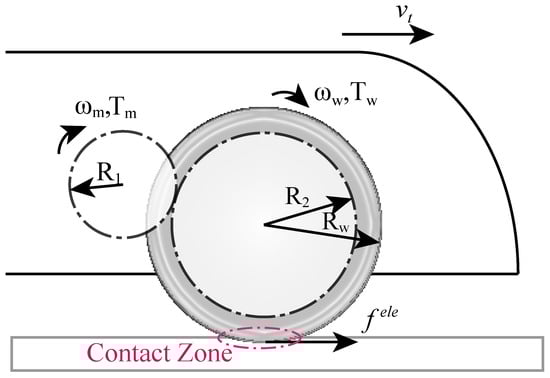
Figure 1. The train adopts a single-axle drive system, where the traction motor’s output torque $T_m$ is transmitted through the gearbox to generate driving torque $T_w$ on the wheels. This interaction with the rail surface creates creep force $f_{ele}$, driving the train forward.

A force analysis of the entire vehicle reveals that the train satisfies the following equation of motion:

$$f^{ele}-f^{dra}-f^{gra}=M{\displaystyle \frac{dv}{dt}},$$

(1)

where the $f^{ele}$ represents the traction force (+) or regenerative braking force (−) of the train, which is capable of avoiding the simultaneous occurrence of traction force and regenerative braking force. It is also the wheel–rail adhesion force. The $f^{dra}$ is the basic resistance to the train’s motion, $f^{gra}=Mg\Delta H$ is the gravitational resistance, M stands for the total mass of the train, g is the gravitational acceleration, and v is the train’s operating speed.

Due to the presence of creep phenomena, there is a discrepancy between the linear velocity of the wheel set and the train’s speed. Therefore, an additional force analysis is conducted specifically for the wheels. To facilitate analysis and calculation, and to maintain consistency with the overall vehicle dynamics model, all driving torques and moments of inertia of the dynamic wheels are consolidated, yielding the following equation:

$$T_w-f^{ele}{R}_w=J_w{\displaystyle \frac{d{\omega }_w}{dt}},$$

(2)

where the $T_w$ is the sum of the driving torques of all the powered wheels, $R_w$ is the radius of the wheels, $J_w$ is the total moment of inertia of the wheels, and ${\omega }_w$ is the angular velocity of the wheels. The transmission ratio of the EMU gearbox is related to the pitch circle radii of the driving gear and the driven gear, which can be determined during the design phase. Consequently, the relationship between the motor output torque $T_m$ and the driving torque of the powered wheels $T_w$ is as follows:

$$T_w=T_m\times R_g,$$

(3)

where $R_g$ is the ratio of the gearbox, and $R_g=R_2/R_1$. From this, the dynamic equation of the motor can be derived as follows:

$$T_m-f^{ele}{\displaystyle \frac{R_w}{R_g}}=J_m{\displaystyle \frac{d{\omega }_m}{dt}}.$$

(4)

The mechanism of wheel–rail adhesion in high-speed trains is complex, exhibiting high nonlinearity and uncertainty. It is typically described using adhesion characteristic curves. Similar to the definition of Coulomb friction, the ratio of the adhesion force $f^{ele}$ to the axle load Q is referred to as the adhesion coefficient $\mu$. Thus, the definition of the adhesion coefficient is given by:

$$\mu ={\displaystyle \frac{f^{ele}}{Q}}.$$

(5)

The adhesion coefficient is influenced by factors such as train speed and rail surface conditions. For high-speed trains, due to their higher operating speeds and more complex running conditions, a more conservative strategy is typically adopted when calculating the adhesion coefficient. Based on extensive adhesion experiments conducted by experts and scholars [34,35,36,37,38], an empirical formula describing the relationship between the adhesion coefficient and creep speed can be derived as follows:

$$\gamma =\left\{\begin{array}{cc}{C}_c{e}^{-C_a{v}_s}-C_d{e}^{-C_b{v}_s},& v_s\ge 0\\ -C_c{e}^{-C_a{v}_s}+C_d{e}^{-C_b{v}_s},& v_s<0\end{array}\right.$$

(6)

where the $C_a$, $C_b$, $C_c$ and $C_d$ are the constant coefficients of the empirical formula, which are related to factors such as rail surface conditions and train speed. To account for the influence of both train speed and creep speed simultaneously, the empirical formula is modified. Since the adhesion coefficient decreases with increasing train speed, a decay factor related to train speed is introduced. The modified formula is expressed as follows:

$$\mu =\left\{\begin{array}{cc}\psi \times (C_c{e}^{-C_a{v}_s}-C_d{e}^{-C_b{v}_s}),& v_s\ge 0\\ \psi \times (-C_c{e}^{-C_a{v}_s}+C_d{e}^{-C_b{v}_s}),& v_s<0\end{array}\right.$$

(7)

where the $\psi$ represents the decay rate of the adhesion coefficient with respect to train speed, derived from an empirical formula that accounts for the relationship between the creep coefficient and speed. The expression for $\psi$ is as follows:

$$\psi =(C_1+{\displaystyle \frac{C_2}{C_3+v}})/max(C_1+{\displaystyle \frac{C_2}{C_3+v}}).$$

(8)

Therefore, the wheel–rail adhesion characteristic of the high-speed railways can be obtained as shown in Figure 2.

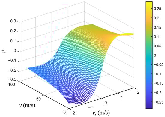
Figure 2. The wheel–rail adhesion characteristic surface of high-speed railways. Based on the conventional empirical formula, the influence coefficient of speed was introduced, that is, the relationship among the adhesion coefficient $\mu$, creepage speed $v_s$ and the train speed v was taken into account.

3. Nonlinear Optimization Model

To accurately reflect speed limits and gradient information, the optimization model is implemented in the spatial domain. First, the total distance D between two adjacent stations is discretized into N segments, where the length of the i-th segment is denoted as $D_i$. To ensure computational efficiency, the value of N should not be excessively large. To avoid overshooting speed limits during optimization due to uniform distance partitioning, a two-level partitioning method is adopted. Specifically, the total distance D is initially divided into several speed limit intervals based on speed transition points. Each interval is then further subdivided into smaller segments $D_i$ proportionally to its length. This can be expressed as $D={\sum }_{i=1}^N{D}_i$. In this section, factors such as train punctuality, safety, motor characteristics, and hybrid braking performance are taken into account. Additionally, to incorporate the influence of wheel–rail coupling dynamics, relevant constraints related to wheel–rail interaction characteristics are introduced.

To ensure the train operates in a timely manner and meets the scheduled time, a punctuality constraint is established; it can be expressed as:

$$T=\sum _{i=1}^N{\displaystyle \frac{D_i}{v_i}},$$

(9)

where $v_i$ represents the velocity over the i-th distance segment, and T is the total travel time. This constraint ensures that the train adheres to the required schedule by accounting for variations in speed across different segments of the route.

During the train’s operation, it experiences various resistance forces that impede its motion, such as bearing friction and the air resistance acting on the front of the train. These forces are commonly modeled using the Davis formula, which provides a mathematical description of the basic resistance encountered during movement. The drag force is given by:

$$f_i^{\mathrm{dra}}=A+B{v}_i+C{v}_i^2,$$

(10)

where $f_i^{\mathrm{dra}}$ is the drag force, and A, B, and C are the Davis coefficients. These coefficients are typically determined through experimental trials.

The train’s operating speed is subject to speed restrictions imposed by the Automatic Train Protection (ATP) system, which ensures the safety of the train’s operation. To maintain compliance with these speed limits, the train’s operating speed at any given segment must remain below the specified speed limit. The speed constraints are defined as:

$$\begin{array}{cc}\hfill & v_i\le V_i^{\lim },\hfill \end{array}$$

(11)

$$\begin{array}{cc}\hfill & v_0=v_N=0.\hfill \end{array}$$

(12)

Here, $V_i^{\lim }$ represents the speed limit at the i-th segment, and the conditions $v_0=v_N=0$ indicate that the train starts and ends at zero velocity, ensuring that the train does not violate the speed constraints at the beginning or end of its journey.

In the operation of the train, the energy balance constraint accounts for the various forms of energy involved, such as electrical energy, kinetic energy, and thermal energy. The energy conservation law can be expressed as:

$$f_i^{ele}{D}_i+f_i^{\mathrm{mec}}{D}_i={\displaystyle \frac{M}{2}}(v_i^2-v_{i-1}^2)+f_i^{\mathrm{dra}}{D}_i+Mg\Delta H_i,$$

(13)

where $f_i^{\mathrm{mec}}$ represents the mechanical braking force, and $f_i^{\mathrm{dra}}$ is the drag force. It ensures that all forms of energy are accounted for, including the energy required for braking, overcoming drag, and counteracting gravitational forces as the train changes altitude.

For the interaction between the wheels and rails, the energy generated by the motor is converted into the kinetic energy of the wheel set and the traction energy of the train. This energy conversion process is expressed as:

$$\begin{array}{cc}\hfill & T_i^m{R}_g{\theta }_i-f_i^{ele}{R}_w{\theta }_i={\displaystyle \frac{J_w}{2}}({\omega }_i^2-{\omega }_{i-1}^2),\hfill \end{array}$$

(14)

$$\begin{array}{cc}\hfill & {\theta }_i={\displaystyle \frac{D_i}{v_i}}\times {\displaystyle \frac{({\omega }_i+{\omega }_{i-1})}{2}}\approx {\displaystyle \frac{D_i}{R_w}}.\hfill \end{array}$$

(15)

Here, ${\theta }_i$ is the angular displacement, ${\omega }_i$ represents the angular velocity of the wheels, and $R_w$ is the radius of the wheels. These equations describe the dynamic energy exchange between the motor and the wheels as the train moves along the track.

The adhesion force between the train’s wheels and the rails plays a crucial role in determining the train’s traction. This force is primarily influenced by the adhesion coefficient, which depends on both the train’s operating speed and the creep speed, and it can be expressed as:

$${\mu }_i={\psi }_i\times {\gamma }_i,$$

(16)

$${\gamma }_i=\left\{\begin{array}{cc}{C}_c{e}^{-C_a{v}_{s,i}}-C_d{e}^{-C_b{v}_{s,i}},\hfill & v_{s,i}\ge 0\hfill \\ -C_c{e}^{-C_a{v}_{s,i}}+C_d{e}^{-C_b{v}_{s,i}},\hfill & v_{s,i}<0\hfill \end{array}\right.$$

(17)

$${\psi }_i={\displaystyle \frac{C_1+\frac{C_2}{C_3+v_i}}{max(C_1+\frac{C_2}{C_3+v_i})}}.$$

(18)

The creep speed $v_{s,i}$ is related to the train’s speed and the wheel’s rotational speed by the equation:

$$v_{s,i}={\omega }_i{R}_w-v_i.$$

(19)

Given that the actual rail surface conditions are far more complex and unpredictable than the model considered here, it is impractical to precisely model the wheel–rail interaction in the optimization model. Therefore, a conservative optimization strategy is employed, assuming a ’wet rail mode’ by introducing a safety factor k. The relationship between the adhesion force and the adhesion coefficient is then expressed as:

$$f_i^{ele}=k{\mu }_{i}Wg,$$

(20)

where W is the axle load. And the safety factor k is introduced to compensate for the uncertainties in rail surface conditions, such as variations in the coefficient of friction, humidity, and surface roughness. Increasing the value of k makes the model more conservative, thereby reducing the operational risk of the train under uncertain rail surface conditions. Specifically, a higher value of k causes the optimization process to prioritize safety margins, reducing the risk of insufficient traction due to fluctuations in the coefficient of friction or slippery surfaces. However, excessively increasing k could lead to a decrease in energy efficiency in the optimization results, as the conservative strategy restricts the operational efficiency of the train, thereby increasing energy consumption. Therefore, the justification for increasing k must balance the relationship between system safety and energy efficiency.

High-speed railways typically use a hybrid braking system, which combines regenerative electric braking and mechanical braking. Regenerative braking is prioritized, and mechanical braking is applied when the regenerative system alone cannot meet the required braking force. The mechanical braking force is always negative and is constrained by the minimum braking performance capability of the train:

$$F_{\max }^{\mathrm{mb}}\le f_i^{\mathrm{mec}}\le 0.$$

(21)

The efficiency of the traction system is governed by the electrical energy output of the motor. During the traction phase, the energy output is positive, while in the regenerative braking phase, it is negative. The efficiency constraints for both the traction and braking phases are expressed as follows:

$$e_i\ge {\displaystyle \frac{T_i^m{R}_g{D}_i}{{\Theta }^{\mathrm{tra}}{R}_w}},$$

(22)

$$e_i\ge {\displaystyle \frac{T_i^m{R}_g{D}_i{\Theta }^{\mathrm{bra}}}{R_w}}.$$

(23)

The traction process of the train is constrained by the motor’s maximum traction force $F_{\max }^{\mathrm{tra}}$ and maximum traction power $P_{\max }^{\mathrm{tra}}$, while the regenerative braking process is constrained by the maximum regenerative braking force $F_{\max }^{\mathrm{rb}}$ and maximum regenerative braking power $P_{\max }^{\mathrm{rb}}$:

$$F_{\max }^{\mathrm{rb}}\le {\displaystyle \frac{T_i^m{R}_g}{R_w}}\le F_{\max }^{\mathrm{tra}},$$

(24)

$${\displaystyle \frac{P_{\max }^{\mathrm{rb}}}{v_i}}\le {\displaystyle \frac{T_i^m{R}_g}{R_w}}\le {\displaystyle \frac{P_{\max }^{\mathrm{tra}}}{v_i}}.$$

(25)

The objective of the proposed optimization model is to minimize the total net energy consumption over all segments:

$$min\sum _{i=1}^N{e}_i.$$

(26)

4. Model Relaxation and Convexity

4.1. Equation Relaxation

The model includes numerous nonlinear constraints, making the optimization problem computationally challenging. According to the second-order conditions of convex optimization, Equations (9), (10), (13)–(18), and (25) are non-convex due to the presence of nonlinear terms, such as $v^2$, $1/v$, and ${\omega }^2$. Drawing from previous research [10], auxiliary variables are introduced to relax the constraints and replace the original nonlinear terms, which significantly improves the computational speed of the model. Specifically, in Equations (9), (10), (13)–(18), and (25), $\alpha$ is introduced to replace $1/v$, ${\beta }^v$ to replace $v^2$, and ${\beta }^{\omega }$ to replace ${\omega }^2$. The following relationships are established:

$${\alpha }_i\ge 1/v_i,$$

(27)

$${\beta }_i^v\ge v_i^2,$$

(28)

$${\beta }_i^{\omega }\ge {\omega }_i^2.$$

(29)

Moreover, the auxiliary variable ${\beta }_i^v$ should also comply with the speed limit, which can replace the constraint constraint (3):

$${\beta }_i^v\le {\left(V_i^{\lim }\right)}^2,$$

(30)

$${\beta }_0^v={\beta }_N^v=0.$$

(31)

According to the analysis in [10], (27) can be transformed to ${\alpha }_i+v_i\ge \sqrt{2^2+{({\alpha }_i-v_i)}^2}$, which is a standard second-order cone programming constraint. The functions corresponding to (28) and (29) are $f=v^2-\beta (\beta >0,v>0)$; then the Hessian matrix of f is:

$$H=\left[\begin{array}{cc}2& 0\\ 0& 0\end{array}\right].$$

(32)

It can be observed that the feasible sets introduced by the three inequalities are both convex sets. Therefore, constraints (9), (10), (13), (3) and (25) can be transformed into:

$$T=\sum _{i=1}^N{D}_i{\alpha }_i,$$

(33)

$$f_i^{\mathrm{dra}}=A+B{v}_i+C{\beta }_i^v$$

(34)

$$f_i^{ele}{D}_i+f_i^{mec}{D}_i={\displaystyle \frac{M}{2}}({\beta }_i^v-{\beta }_{i-1}^v)+f_i^{dra}{D}_i+Mg\Delta H_i$$

(35)

$$T_i^m{R}_g{D}_i/R_w-f_i^{ele}{R}_w{D}_i/R_w={\displaystyle \frac{J_w}{2}}({\beta }_i^{\omega }-{\beta }_{i-1}^{\omega })$$

(36)

$$P_{\max }^{\mathrm{rb}}{\alpha }_i\le f_i^{\mathrm{ele}}\le P_{\max }^{\mathrm{tra}}{\alpha }_i$$

(37)

Additionally, $\psi$ can be approximated using a second-order fitting method, transforming (18) into a quadratic polynomial:

$${\psi }_i=p_1{v}_i^2+p_2{v}_i+p_3=p_1{\beta }_i^v+p_2{v}_i+p_3,$$

(38)

where the $p_1$, $p_2$ and $p_3$ are the constant coefficients of the fitted quadratic polynomial. Similarly, since the creep speed during the operation of high-speed railways is relatively small, (17) can be approximated by a first-order polynomial:

$${\gamma }_i=p_0{v}_{s,i},$$

(39)

where the $p_0$ is the constant coefficient.

4.2. Tightened McCormick Envelope

Constraint (16) contains bilinear terms. In this paper, the McCormick envelope approximation method is employed to transform it into four linear inequality constraints:

$$\begin{array}{c}\hfill \left\{\begin{array}{c}{\mu }_i\ge {\Psi }_L{\gamma }_i+{\Gamma }_L{\psi }_i+{\Psi }_L{\Gamma }_L,\\ {\mu }_i\ge {\Psi }_U{\gamma }_i+{\Gamma }_U{\psi }_i+{\Psi }_U{\Gamma }_U,\\ {\mu }_i\le {\Psi }_U{\gamma }_i+{\Gamma }_L{\psi }_i+{\Psi }_U{\Gamma }_L,\\ {\mu }_i\le {\Psi }_L{\gamma }_i+{\Gamma }_U{\psi }_i+{\Psi }_L{\Gamma }_U.\end{array}\right.\end{array}$$

(40)

The ${\Psi }_U$ and ${\Psi }_L$ represent the upper and lower bounds of $\psi$ respectively, and the ${\Gamma }_U$ and ${\Gamma }_L$ represent the upper and lower bounds of $\gamma$ respectively. The precision of McCormick relaxations is governed by the tightness of their bounds, which should be tightened as much as possible. Initial boundary values derived from the known boundary conditions of the model often lead to overly relaxed constraints, compromising the accuracy of bilinear term estimates. To enhance the precision of McCormick envelope approximations, this paper further proposes a tightened McCormick envelope method. A pre-optimization approach is employed to determine tighter and more appropriate boundary values through specific iterative rules, with the implementation workflow detailed in Figure 3.

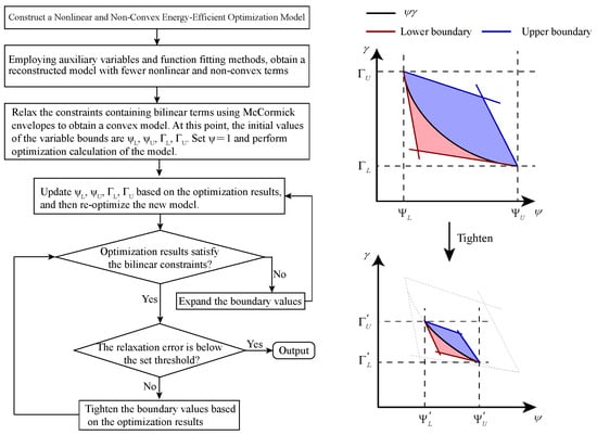
Figure 3. Implementation of the Tightened McCormick Envelope Method and schematic diagram. The method employs model reconstruction and the McCormick approach to transform the model into a convex form. Additionally, heuristic rules are applied to tighten the bounds of the McCormick envelopes.

The relaxation of (27) and (28) converges to equality, which indicates that the model is accurate and valid without compromising optimality, as proven in [10]. To ensure that Equation (29) also converges to an equality, a penalty term is added to the objective function, modifying it as follows:

$$min(\sum _{i=1}^N{e}_i+\lambda \sum _{i=1}^N{\beta }_i^{\omega }),$$

(41)

where $\lambda$ is a tuning factor used to adjust the magnitude of the penalty term introduced by the relaxation variable. Its role is to ensure that this penalty term aligns with the scale of the original objective function, as defined in Equation (26), while keeping the relaxation error associated with ${\omega }^2$ below a threshold of 0.01%. In this study, if $\lambda$ is set too small, the relaxation error related to ${\omega }^2$ becomes significantly large; conversely, if $\lambda$ is too large, it diminishes the weight of the energy-saving objective within the overall function. Therefore, the approach for determining $\lambda$ is to select the smallest possible value that maintains a desired balance between relaxation error and energy-saving performance. To this end, simulations were conducted for $\lambda$ ranging from 60 to 160, ultimately leading to the selection of 120 as the optimal value. When $\lambda$ exceeds 120, the energy-saving performance of the train in the simulation case fluctuates by approximately 0.1%, and for values between 130 and 160, the relaxation error associated with ${\omega }^2$ even increases to 0.04%. When $\lambda$ falls below 120, similar fluctuations of about 0.1% in energy-saving performance are observed, while the relaxation error also rises—reaching 0.04% at $\lambda =60$.

5. Results and Discussion

In this section, a comparison between the two models is conducted to evaluate the energy-efficient train driving strategy that considers wheel–rail adhesion characteristics. Model 1 represents the traditional EETC model, which equates the motor output to the actual traction force of the train. Model 2 is the EETC model that incorporates wheel–rail adhesion characteristics. Specifically, Model 2 and Model 1 are designed for wet and dry track conditions, respectively, and the train driving mode can be switched based on the operational environment information. Using the parameters of the Chinese CRH3800AL high-speed railways listed in Table 1, two numerical experiment cases are proposed. Case 1 is a complex scenario based on real-world high-speed rail line data in China, comparing the speed trajectory optimization of Model 1 and Model 2 under both wet and dry track conditions, aiming to validate the accuracy and effectiveness of the models in practical situations. Case 2 compares the speed tracking control of Model 1 and Model 2 on wet road sections, aiming to validate the safety and energy-saving advantages of the proposed model.

Table 1. Vehicle Specification Parameters of Train CRH380AL and Journey Information.

Parameter	Value	Parameter	Value
$F_{\max }^{\mathrm{tra}}$ (kN)	520	M (t)	890
$F_{\max }^{\mathrm{rb}}$ (kN)	−520	W (t)	756
$P_{\max }^{\mathrm{tra}}$ (kW)	20,440	A (N)	5200
$P_{\max }^{\mathrm{rb}}$ (kW)	−20,440	B (N·h/km)	25.35
$F_{\max }^{\mathrm{mec}}$ (kN)	−800	C (N·h2/km2)	1.084
$F_{\max }^{\mathrm{cou}}$ (kN)	980	${\Theta }^{\mathrm{tra}}$	0.9
D (km)	127	${\Theta }^{\mathrm{bra}}$	0.6
$J_w$ (kg·m2)	4480	$R_w$	0.41

All numerical experiments were conducted on a computer equipped with a 12th Gen Intel(R) Core(TM) i7-12700F 2.10 GHz processor and 16GB RAM. The optimization solver used in this paper is Gurobi 11.0.2, and optimization computations were performed based on its internal homogeneous bar grid algorithm. The speed tracking control simulation in Case 2 was implemented in Matlab/Simulink. Due to the influence of rail surface conditions on wheel–rail adhesion characteristics, the values of the adhesion coefficient under dry and wet rail conditions are shown in Table 2. This paper utilizes the fitting toolbox of MATLAB R2022b to obtain the fitting parameters. The polynomial fitting results are shown in Table 3. The adjustment factor $\lambda$ is set to 120 in the numerical simulations to ensure that the penalty term in the objective function is of the same order of magnitude as the total energy consumption of the train.

Table 2. The values of adhesion coefficients under different orbital conditions.

	${\mathit{C}}_1$	${\mathit{C}}_2$	${\mathit{C}}_3$	${\mathit{C}}_{\mathit{a}}$	${\mathit{C}}_{\mathit{b}}$	${\mathit{C}}_{\mathit{c}}$	${\mathit{C}}_{\mathit{d}}$
Dry	0.06	46.6	260	0.54	1.2	1.0	1.0
Wet	0.04	13.7	120	0.19	0.54	0.4	0.4

Table 3. Fitting results based on MATLAB toolbox.

	${\mathit{p}}_0$	${\mathit{R}}^2$	${\mathit{p}}_1$	${\mathit{p}}_2$	${\mathit{p}}_3$	${\mathit{R}}^2$
dry rail conditions	0.5438	0.997	4.1466$\times {10}^{-5}$	−0.008	0.9866	0.999
wet rail conditions	0.1253	0.999	8.0335$\times {10}^{-5}$	−0.012	0.9522	0.990

To ensure the safety of the model, the safety factor k is set to 0.9. Based on the train’s speed limit information and wheel–rail adhesion characteristics, the upper and lower bounds of $\psi$ and $\gamma$ can be calculated. In this case, the maximum speed limit of the train is 300 km/h, and the region where $v_s<2$ m/s is considered the stable region for adhesion characteristics. Therefore, the initial values are ${\Psi }_U=1$, ${\Psi }_L=0.5986$, ${\Gamma }_U=0.2862$, and ${\Gamma }_L=-0.2862$. After applying the tightening calculation, the revised boundary values are ${\Psi }_U=0.9860$, ${\Psi }_L=0.5986$, ${\Gamma }_U=0.0725$, and ${\Gamma }_L=-0.1270$.

These boundary values, including the upper and lower bounds for $\psi$ and $\gamma$, are derived using the process outlined in Figure 3, which details the relaxation method and the calculation of wheel–rail adhesion limits. The initial values of these parameters reflect typical operating conditions, while the tightening process ensures that the optimization problem remains consistent with the real-world behavior of wheel–rail interaction. The revised values, after tightening, ensure the stability of the optimization process and contribute to the overall safety and performance of the proposed model.

5.1. Optimization in Real-Line Scenarios

This case utilizes real-world operational data from a Chinese high-speed train, incorporating gradients and ATP speed limit information during the train’s operation. Numerical simulation experiments were conducted for both dry and wet rail conditions using the two models. Figure 4 presents a comparison of the optimal speed trajectories and traction/braking force curves for both models. Figure 5 shows the relaxation errors of the models.

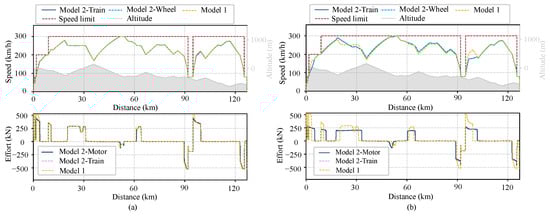
Figure 4. Speed and traction/braking curves of the train in Case 1: (a) dry rail conditions; (b) wet rail conditions.

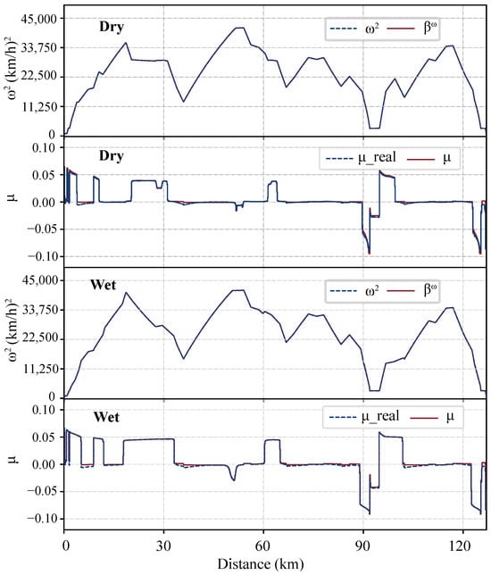
Figure 5. Comparison of auxiliary variables ${\beta }^{\omega }$ and $\mu$ with Original Variables ${\omega }^2$ and the real $\mu$ value which is calculated based on the model in Case 1. The red line and the blue dotted line basically coincide.

5.1.1. Driving Strategy

In Figure 4, Model 2 adopts a strategy that distinguishes between train speed and wheel speed, and does not equate the motor output with the actual traction force of the train, in order to better account for the impact of wheel–rail characteristics on train performance. Specifically, Model 2: Train refers to the motion state of the entire train, typically described by the overall train speed, while Model 2: Wheel refers to the motion state of the individual wheels, reflecting the wheel speed, which may differ from the overall train speed, particularly when considering wheel–rail contact characteristics. Meanwhile, Model 2: Motor refers to the traction force output by the traction motor, while Model 2: Train represents the actual traction force of the train.

As shown in Figure 4, under dry rail conditions, the optimal speed trajectories of the two models largely overlap. The maximum traction/braking force of the train is influenced by the rail surface conditions when wheel–rail characteristics are considered, and it is lower than the maximum traction/braking force under conventional ideal conditions. Additionally, due to the presence of creep between the wheel and rail, the linear speed of the motor is slightly greater than the train speed during the traction phase, resulting in a positive creep speed. Conversely, during the braking phase, the motor’s linear speed is less than the train speed, leading to a negative creep speed. When wheel–rail creep is considered, Model 2 adopts a lower maximum traction force, as seen in the 0–4 km and 95–100 km segments.

Under wet conditions, the maximum traction and braking forces of the train are constrained by the maximum adhesion force. Consequently, the train employs longer traction and braking distances to ensure punctuality. Furthermore, based on the analysis of wheel–rail adhesion characteristics, the maximum adhesion force decreases as the train speed increases. This results in a slight reduction in traction force during acceleration phases (e.g., the first two traction phases) and a slight increase in traction force during deceleration phases (e.g., the 20–33 km segment) as the distance progresses.

5.1.2. Total Energy Consumption

The solution results of the two models are shown in Table 4. It can be seen that the computation times for the proposed model are 1.22 s and 1.26 s, respectively. Although the computation time has increased compared to the original Model 1, which does not incorporate wheel–rail adhesion characteristics, the proposed model still maintains a high computational efficiency.

Table 4. CPU Time and Net Energy Consumption of Train Operation in Case 2.

	Model 1	Model 2-Dry	Model 2-Wet
Energy (kWh)	1650.51	1669.26	1773.17
CPU time (s)	0.84	1.22	1.26

In normal rail conditions, Model 1 consumes a total of 1650.51 kWh, while Model 2 consumes 1669.26 kWh. This discrepancy can be attributed to the fact that Model 1 does not account for the energy losses associated with traction force transmission between the wheel and rail, resulting in a higher energy consumption for Model 2 in comparison to Model 1.

In wet conditions, Model 1 does not take into account the impact of wheel–rail characteristics, meaning that its driving strategy and energy consumption are not affected by rail surface conditions. In contrast, Model 2 incorporates wheel–rail creep characteristics into consideration, thereby sacrificing certain energy efficiency to ensure a safer driving strategy, resulting in a 6.22% increase in energy consumption compared to normal rail conditions.

5.1.3. Model Accuracy Verification

Model 2 employs a convexification approach that introduces auxiliary variables and utilizes the McCormick envelope approximation. The relaxation accuracy of $\alpha$ and ${\beta }^v$ has already been validated [10]. This paper primarily analyzes the relaxation errors of constraints (29) and (40). As shown in Figure 5, when the auxiliary variables are nearly equal to the original variables, the model can be considered to have good accuracy. To improve the precision of the McCormick envelope, this study also proposes a tightened McCormick envelope method. The performance is evaluated using both average error and maximum error metrics, as presented in Table 5. The errors are calculated through the following equations:

$$\begin{array}{c}\hfill er{r}_{ave}={\displaystyle \frac{{\sum }_{i=1}^N|{\mu }_i-{\mu }_{real,i}|}{{N\left|\mu \right|}_{max}}},\end{array}$$

(42)

$$\begin{array}{c}\hfill er{r}_{max}=\underset{1\le i\le N}{max}{\displaystyle \frac{|{\mu }_i-{\mu }_{real,i}|}{{\left|\mu \right|}_{max}}},\end{array}$$

(43)

where the ${\left|\mu \right|}_{max}$ represents the largest value of $|{\mu }_i|$ among $i=1,2,\dots ,N$. Compared to the standard McCormick envelope method, the tightened approach reduces the average error by 7.6% and the maximum error by 25.49%. As shown in Figure 5, deviations in $\mu$ primarily occur in braking regions, where the estimated values are smaller (i.e., larger in absolute magnitude) than those calculated using empirical formulas. This implies a slight overestimation of the adhesion force under the same creep speed and train velocity during braking, with a maximum relative error of 9.61%, leading to an overly optimistic control strategy. However, by introducing a safety factor of k, the adhesion force calculation remains conservative even at the maximum error point. This demonstrates the accuracy and reliability of the proposed model.

Table 5. The maximum error and average error of the model in Case 2.

Relaxation Method	${\mathit{err}}_{\mathit{ave}}$	${\mathit{err}}_{\mathit{max}}$
McCormick	9.39%	35.1%
Tightened McCormick	1.79%	9.61%

5.2. Speed Tracking Control Simulation

This case compares the driving strategy proposed in this paper with a conventional anti-slip control strategy. The traditional anti-slip control strategy is simulated using MATLAB R2022b, where a train anti-slip controller based on the classical combined correction method is implemented. In this case, an ideal slip observer is adopted under the assumption that transitions in rail surface conditions (e.g., dry to wet) can be rapidly detected, enabling immediate anti-slip interventions. Specifically, when slip is predicted, the torque is instantaneously reduced to 20% of its original value. The experiment designates the 20.5–55 km segment as a wet rail section, with the remaining sections as dry rail. To evaluate the superiority of the proposed driving strategy in terms of both safety and energy efficiency, two train operation simulation models were developed.

Model 2 is specifically designed for the wet track mode, which is activated based on monitoring information of the track surface conditions during train operation, but the mode itself does not have detection capabilities and relies on real-time condition information. In this mode, the model employs a conservative control strategy for traction and braking forces, effectively preventing wheel slip even under slippery conditions, while minimizing energy consumption to the greatest extent. This switching mechanism enables the control strategy to be flexibly adjusted in response to varying track conditions, thereby enhancing both the system’s safety and energy efficiency.

The specifications of these models are as follows:

• Model 1: The speed profile generated by the conventional EETC strategy was adopted as the target speed trajectory, with the speed tracking control implemented using a conventional feedforward and feedback controller.
• Model 2: The speed profile generated by the proposed new driving strategy was adopted as the target speed trajectory, with speed tracking control implemented using a conventional feedforward and feedback controller.

The speed trajectories of the train under both strategies are illustrated in Figure 6.

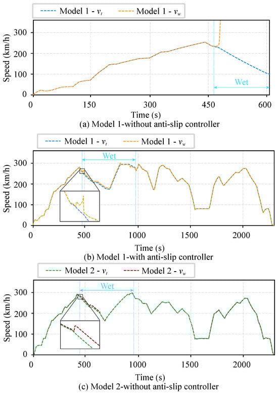
Figure 6. Speed trajectory curves in Case 2. During the 20.5–55 km (about 460–980 s) interval, the train operates on a wet rail section.

5.2.1. Driving Safety

When tracking the speed profile obtained by the conventional EETC strategy without a slip control system, the train experiences severe wheel slip conditions, as illustrated in Figure 6a. Upon entering wet track sections, the linear velocity of the wheel increases rapidly, causing intense friction between the wheels and the rails that compromises operational safety and induces irreversible damage to both components.

The implementation of a slip control system effectively mitigates these hazardous phenomena, as demonstrated in Figure 6b. The controller activates when wheel linear velocity surges, suppressing motor output torque to restore velocity within safe limits and prevent prolonged slipping. However, due to inherent detection latency, this reactive approach still permits localized wheel–rail slip occurrences (see zoomed region in Figure 6b), which may accelerate wear and reduce service life.

In contrast to this passive regulation method, the proposed strategy proactively reduces traction force through predictive optimization, significantly diminishing slip risks (Figure 6c). During transitions from dry to wet conditions, the linear velocity of the wheel remains stable within safe boundaries without slip incidents, ensuring both operational safety and stability of the ride.

5.2.2. Driving Energy Efficiency

The control strategy depicted in Figure 6b, while ensuring operational safety, results in significant deviation of the actual speed profile from the originally optimized trajectory, leading to substantially increased energy consumption. As shown in Table 6, the simulation results indicate a total net energy consumption of 2832 kWh for this case.

Table 6. Energy Consumption of Train Control.

	Model 1	Model 1-with Anti-Slip Controller	Model 2
Energy (kWh)	∖	2832	2280

In contrast, the driving strategy presented in Figure 6c proactively accounts for adverse rail conditions through predictive optimization to prevent wheel slip. As shown in Table 6, this approach yields a total net energy consumption of 2280 kWh in the same scenario. Compared to traditional methods that combine slip control and EETC, the proposed strategy eliminates wheel slip, allowing the actual speed curve to closely follow the optimized speed curve. As a result, it reduces energy consumption by 552 kWh, achieving a 19.49% energy savings compared to the traditional EETC method with slip control, demonstrating superior performance in both safety and energy efficiency. However, it must be acknowledged that the benchmark model we compared is the ideal slip controller, which is relatively conservative.

6. Conclusions

This paper presents an EETC model for high-speed trains that incorporates wheel–rail interaction safety constraints. The model uses equation relaxation, curve fitting, and tightened McCormick envelope methods to reformulate the original nonlinear non-convex model into a convex one, reducing computational complexity. Compared to conventional EETC, the proposed model takes a more conservative approach to traction and braking, selecting appropriate traction forces to prevent wheel–rail slippage in both wet and dry conditions. Numerical simulations were conducted on the CRH380AL high-speed train on the Guiyang North–Kaili South route. The results demonstrate that the proposed method effectively prevents wheel slip through global optimization while ensuring operational safety and achieving a 19.49% reduction in energy consumption. Additionally, while the adhesion model used in this study enhances accuracy, it is based on empirical fitting and may not fully capture localized or temporary variations in adhesion, such as those caused by patches of oil or varying moisture conditions. Future work will address this limitation to improve the model’s responsiveness to such transient changes.

The model proposed in this paper, while primarily developed and validated through theoretical modeling and simulation, is designed with clear potential for real-time implementation. By employing convex optimization—specifically a Second-Order Cone Programming (SOCP) formulation—along with tailored relaxation techniques, the model achieves reduced computational complexity and reliable solving efficiency, making it suitable for fast optimization in complex train control tasks. The SOCP structure ensures polynomial-time complexity and scalable performance with respect to the number of track segments N, providing a solid theoretical foundation for real-time application. However, an increase in the number of track segments, N, may still affect computation time, and future research will analyze and optimize this. Ensuring the model’s robustness in real-time applications, such as across different test case scenarios, remains a challenge. Future work will address these issues to ensure stable operation under varying track conditions while maintaining EETC.

Although the model proposed in this paper primarily focuses on the integrated design of all dynamic wheels, the technique has the potential for extension to dispersed power trains, such as the CRH380AL high-speed train. This extension can be achieved by adopting a control strategy that incorporates the characteristics of distributed traction. In such a system, motors are distributed across multiple carriages. By implementing a control strategy that accounts for these distributed traction characteristics, the interactions between carriages, traction force balancing, coordinated control, and dynamic optimization of the traction force can be effectively analyzed. More complex dynamic models and optimization algorithms can be employed to simulate and optimize the operational behavior of distributed power trains. This approach aims to enhance overall energy efficiency and system safety, with future research dedicated to further exploration and optimization in this area.

References

- Yin, J.; Tang, T.; Yang, L.; Xun, J.; Huang, Y.; Gao, Z. Research and development of automatic train operation for railway transportation systems: A survey. Transp. Res. Part C-Emerg. Technol. 2017, 85, 548–572. [Google Scholar] [CrossRef]
- Albrecht, A.; Howlett, P.; Pudney, P.; Vu, X.; Zhou, P. The key principles of optimal train control—Part 1: Formulation of the model, strategies of optimal type, evolutionary lines, location of optimal switching points. Transp. Res. Part B-Methodol. 2016, 94, 482–508. [Google Scholar] [CrossRef]
- Howlett, P.G.; Milroy, I.P.; Pudney, P.J. Energy-efficient train control. Control Eng. Pract. 1994, 2, 193–200. [Google Scholar] [CrossRef]
- Huang, Y.; Zhou, W.; Qin, J.; Deng, L. Optimization of energy-efficiency train schedule considering passenger demand and rolling stock circulation plan of subway line. Energy 2023, 275, 127475. [Google Scholar] [CrossRef]
- Wang, Y.; De Schutter, B.; van den Boom, T.J.J.; Ning, B. Optimal trajectory planning for trains—A pseudospectral method and a mixed integer linear programming approach. Transp. Res. Part C-Emerg. Technol. 2013, 29, 97–114. [Google Scholar] [CrossRef]
- Lu, S.; Wang, M.Q.; Weston, P.; Chen, S.; Yang, J. Partial Train Speed Trajectory Optimization Using Mixed-Integer Linear Programming. IEEE Trans. Intell. Transp. Syst. 2016, 17, 2911–2920. [Google Scholar] [CrossRef]
- Cao, Y.; Zhang, Z.; Cheng, F.; Su, S. Trajectory Optimization for High-Speed Trains via a Mixed Integer Linear Programming Approach. IEEE Trans. Intell. Transp. Syst. 2022, 23, 17666–17676. [Google Scholar] [CrossRef]
- Lu, S.; Hillmansen, S.; Ho, T.K.; Roberts, C. Single-Train Trajectory Optimization. IEEE Trans. Intell. Transp. Syst. 2013, 14, 743–750. [Google Scholar] [CrossRef]
- Su, S.; Wang, X.; Cao, Y.; Yin, J. An Energy-Efficient Train Operation Approach by Integrating the Metro Timetabling and Eco-Driving. IEEE Trans. Intell. Transp. Syst. 2020, 21, 4252–4268. [Google Scholar] [CrossRef]
- Feng, M.; Huang, Y.; Lu, S. Eco-driving Strategy Optimization for High-speed Railways Considering Dynamic Traction System Efficiency. IEEE Trans. Transp. Electrif. 2024, 10, 1617–1627. [Google Scholar] [CrossRef]
- Xiao, Z.; Murgovski, N.; Chen, M.; Feng, X.; Wang, Q.; Sun, P. Eco-Driving for Metro Trains: A Computationally Efficient Approach Using Convex Programming. IEEE Trans. Veh. Technol. 2023, 72, 10063–10076. [Google Scholar] [CrossRef]
- Blanco-Castillo, M.; Fernández-Rodríguez, A.; Fernández-Cardador, A.; Cucala, A. Eco-Driving in Railway Lines Considering the Uncertainty Associated with Climatological Conditions. Sustainability 2022, 14, 8645. [Google Scholar] [CrossRef]
- Domínguez, M.; Fernández-Cardador, A.; Cucala, A.; Gonsalves, T.; Fernández, A. Multi objective particle swarm optimization algorithm for the design of efficient ATO speed profiles in metro lines. Eng. Appl. Artif. Intell. 2014, 29, 43–53. [Google Scholar] [CrossRef]
- Shang, M.; Zhou, Y.; Mei, Y.; Zhao, J.; Fujita, H. Energy-Saving Train Operation Synergy Based on Multi-Agent Deep Reinforcement Learning on Spark Cloud. IEEE Trans. Veh. Technol. 2023, 72, 214–226. [Google Scholar] [CrossRef]
- Zhou, K.; Song, S.; Xue, A.; You, K.; Wu, H. Smart Train Operation Algorithms Based on Expert Knowledge and Reinforcement Learning. IEEE Trans. Syst. Man, Cybern. Syst. 2022, 52, 716–727. [Google Scholar] [CrossRef]
- Cheng, R.; Yu, W.; Song, Y.; Chen, D.; Ma, X.; Cheng, Y. Intelligent Safe Driving Methods Based on Hybrid Automata and Ensemble CART Algorithms for Multihigh-Speed Trains. IEEE Trans. Cybern. 2019, 49, 3816–3826. [Google Scholar] [CrossRef]
- Nold, M.; Corman, F. Increasing realism in modelling energy losses in railway vehicles and their impact to energy-efficient train control. Railw. Eng. Sci. 2024, 32, 257–285. [Google Scholar] [CrossRef]
- Peng, Y.; Chen, F.; Chen, F.; Wu, C.; Wang, Q.; He, Z.; Lu, S. Energy-efficient train control: A comparative study based on permanent magnet synchronous motor and induction motor. IEEE Trans. Veh. Technol. 2024, 73, 16148–16159. [Google Scholar] [CrossRef]
- Peng, Y.; Lu, S.; Chen, F.; Liu, X.; Tian, Z. Energy-efficient train control incorporating inherent reduced-power and hybrid braking characteristics of railway vehicles. Transp. Res. Part C Emerg. Technol. 2024, 163, 104626. [Google Scholar] [CrossRef]
- Chang, C.; Chen, B.; Cai, Y.; Wang, J. Experimental investigation of high-speed wheel-rail adhesion characteristics under large creepage and water conditions. Wear 2024, 540–541, 205254. [Google Scholar] [CrossRef]
- Buckley-Johnstone, L.; Trummer, G.; Voltr, P.; Six, K.; Lewis, R. Full-scale testing of low adhesion effects with small amounts of water in the wheel/rail interface. Tribol. Int. 2020, 141, 105907. [Google Scholar] [CrossRef]
- Ma, H.; Niu, Y.; Zou, X.; Zhang, J. Experimental Study of Effects of the Third Medium on the Maximum Friction Coefficient between Wheel and Rail for High-Speed Trains. Shock Vib. 2021, 2021, 6904346. [Google Scholar] [CrossRef]
- Gao, H.; Pfaff, R.; Babilon, K.; Ye, Y. A comprehensive wheel–rail contact model incorporating sand fragments and its application in vehicle braking simulation. Veh. Syst. Dyn. 2024, 63, 2019–2038. [Google Scholar] [CrossRef]
- Krier, P.; White, B.; Ferriday, P.; Watson, M.; Buckley-Johnstone, L.; Lewis, R.; Lanigan, J. Vehicle-based cryogenic rail cleaning: An alternative solution to ‘leaves on the line’. Proc. Inst. Civ. Eng. -Civ. Eng. 2021, 174, 176–182. [Google Scholar] [CrossRef]
- Swan, J.; Radoiu, M. Microwave Plasma System for Continuous Treatment of Railway Track. Technologies 2020, 8, 54. [Google Scholar] [CrossRef]
- Kalker, J. A Fast Algorithm for the Simplified Theory of Rolling Contact. Veh. Syst. Dyn. 1982, 11, 1–13. [Google Scholar] [CrossRef]
- Pombo, J.; Ambrósio, J.; Pereira, M.; Lewis, R.; Dwyer-Joyce, R.; Ariaudo, C.; Kuka, N. Development of a wear prediction tool for steel railway wheels using three alternative wear functions. Wear 2011, 271, 238–245. [Google Scholar] [CrossRef]
- Mei, T.; Li, H. A novel approach for the measurement of absolute train speed. Veh. Syst. Dyn. 2008, 46, 705–715. [Google Scholar] [CrossRef]
- Wang, S.; Xiao, J.; Huang, J.; Sheng, H. Locomotive wheel slip detection based on multi-rate state identification of motor load torque. J. Frankl. Inst. 2016, 353, 521–540. [Google Scholar] [CrossRef]
- Chen, Y.; Dong, H.; Lü, J.; Sun, X.; Guo, L. A Super-Twisting-Like Algorithm and Its Application to Train Operation Control with Optimal Utilization of Adhesion Force. IEEE Trans. Intell. Transp. Syst. 2018, 17, 3035–3044. [Google Scholar] [CrossRef]
- Uyulan, C.; Gokasan, M.; Bogosyan, S. Re-adhesion control strategy based on the optimal slip velocity seeking method. J. Mod. Transp. 2018, 26, 36–48. [Google Scholar] [CrossRef]
- Wu, B.; Xiao, G.; An, B.; Wu, T.; Shen, Q. Numerical study of wheel/rail dynamic interactions for high-speed rail vehicles under low adhesion conditions during traction. Eng. Fail. Anal. 2022, 137, 106266. [Google Scholar] [CrossRef]
- Xiao, G.; Wu, B.; Yao, L.; Shen, Q. The traction behaviour of high-speed train under low adhesion condition. Eng. Fail. Anal. 2022, 131, 105858. [Google Scholar] [CrossRef]
- Spiryagin, M.; Lee, K.S.; Yoo, H.H.; Kashura, O.; Kostyukevich, O. Modeling of adhesion for railway vehicles. J. Adhes. Sci. Technol. 2008, 22, 1017–1034. [Google Scholar] [CrossRef]
- Zhang, W.; Chen, J.; Wu, X.; Jin, X. Wheel/rail adhesion and analysis by using full scale roller rig. Wear 2002, 253, 82–88. [Google Scholar] [CrossRef]
- Yuan, Z.; Wu, M.; Tian, C.; Zhou, J.; Chen, C. A review on the application of friction models in wheel-rail adhesion calculation. Urban Rail Transit 2021, 7, 1–11. [Google Scholar] [CrossRef]
- Polach, O. Creep forces in simulations of traction vehicles running on adhesion limit. Wear 2005, 258, 992–1000. [Google Scholar] [CrossRef]
- Liu, W.; Qi, H.; Huang, J.; Chen, Y.; He, S.; Feng, H. Rail surface identification and adhesion control based on dynamic adhesion characteristics. Discov. Appl. Sci. 2025, 7, 657. [Google Scholar] [CrossRef]
Disclaimer/Publisher’s Note: The statements, opinions and data contained in all publications are solely those of the individual author(s) and contributor(s) and not of MDPI and/or the editor(s). MDPI and/or the editor(s) disclaim responsibility for any injury to people or property resulting from any ideas, methods, instructions or products referred to in the content. |
© 2025 by the authors. Licensee MDPI, Basel, Switzerland. This article is an open access article distributed under the terms and conditions of the Creative Commons Attribution (CC BY) license (https://creativecommons.org/licenses/by/4.0/).