Memory Self-Learning Grey Wolf Optimization for PMSM Parameter Identification with Inverter Voltage-Error Compensation

Abstract

Aiming at the problems of voltage distortion caused by voltage drop nonlinearity of voltage source inverter (VSI) tubes, poor recognition accuracy of traditional grey wolf optimization (GWO) in identifying parameters of permanent magnet synchronous motor (PMSM), and slow convergence speed at the later stage, a memory self-learning grey wolf optimization (MSLGWO) algorithm with voltage error compensation is proposed. First, the output voltage error caused by switching tube voltage drop in different conduction states of the inverter is compensated to mitigate its impact on parameter identification. Then, cat mapping is employed to generate the initial position of the grey wolves, combined with an inverse learning strategy to find and select the superior solution among them to secure the variety of the initial population. In addition, the rate of convergence is accelerated by using a cosine-varying convergence factor to maintain a balance between global and local search capabilities. Lastly, inspired by the particle swarm optimization algorithm, a memory-based self-learning mechanism is incorporated to leverage the past experiences of individual wolves. Compared with traditional GWO, the proposed MSLGWO with voltage compensation reduces the identification error by at least 50.0% and completes the process within 0.11 s.

1. Introduction

Permanent magnet synchronous motors (PMSMs) have been widely employed in various high-precision and high-performance applications, such as electric vehicles, industrial automation, and renewable energy systems, owing to their advantages of excellent control performance, simple structure, and high power density [1,2,3,4]. However, parameter identification for PMSMs remains a critical issue, and accurate parameters are essential for achieving optimal control performance, control prediction, etc. [5]. The degree of magnetic saturation, temperature, and load disturbance during actual operation are only a few of the variables that might affect the PMSM’s parameters, which include stator resistance, cross and straight axis inductance, and permanent magnet flux. The motor’s resistance value changes in response to temperature increases. The permanent magnet flux in the PMSM may be affected by the external magnetic field, and the magnetic saturation may lead to changes in the magnetic flux and inductance. The motor’s control performance will be impacted by the changing settings, and the system may not function properly. Therefore, achieving multi-parameter online PMSM recognition is quite important.

The parameter identification of PMSM is classified into offline identification and online identification. Offline identification methods include the finite element analysis method [6] and the experimental determination method [7]. However, offline identification requires a large amount of data collection and does not take into account the actual working conditions and influencing factors. The online identification algorithm estimates the parameters iteratively in real time by collecting data, including current, voltage speed, etc., which can better reflect the motor working conditions and better real-time performance. Online identification methods include traditional methods such as least squares (LS) [8], extended Kalman filter (EKF) [9], and model reference adaptive method (MRAS) [10], as well as intelligent algorithms that have risen in recent years.

In [11], for the purpose of controlling PMSM current, a real-time, data-driven recursive least squares estimation technique was presented. In [12], the nonlinearity of inverters was taken into consideration, and an online identification solution for PMSMs with dual extended Kalman filters was suggested. A multi-parameter identification method for PMSMs based on MRAS and simulated annealing particle swarm optimization was presented in [13]. The motor control system’s mechanical and electrical parameters were identified and optimized by the algorithm.

Intelligent algorithms are increasingly used in the field of identifying parameters of PMSMs, and a number of algorithms and their optimization methods have been proposed. An enhanced fuzzy PSO algorithm was introduced in [14] to alter each particle’s speed from being solely influenced by the optimum particle to being influenced by the particles in its immediate vicinity. The algorithmic recognition accuracy was increased by this strategy. In [15], two improved PSO schemes were proposed to identify not only the electrical but also the mechanical parameters of the PMSM. In [16], to tackle the issue of parameter recognition’s sensitivity to motor speed, a novel neural network technique with variable step duration was suggested. In [17], together with the development of a built-in PMSM predictive control parameter compensation model, a novel set of four equations was employed for iterative parameter optimization in the Bacterial Foraging Optimization Algorithm. A nonlinear descending technique was applied in [18] to adjust the inertia weights of particle swarms. Although it helped the algorithm perform better in terms of discrimination, it was unable to prevent the search from reaching local optimality. An improved memetic particle swarm optimization that combined PSO and a memetic algorithm was proposed in [19]. In [20], a new weak magnetization scheme and a modified vector controlling strategy were proposed to mitigate the effects of the inverse electromotive force effect. The GWO was used in [21] to improve the proportional-integral controller settings for the speed adaptive law derived from MRAS. In [22], an improved dynamic proportional weighting strategy was introduced to speed up the particle convergence. In [23], methods for updating the position of the leader wolf by the modified sine-cosine algorithm balanced the global and local exploitation capabilities of GWO. Improvements to GWO with hunting groupings and nonlinear convergence factors were proposed in [24]. In [25], global search was improved using the Levy flight strategy with better stability and computational accuracy. In [26], combining the improved GWO with a PID controller enabled precise control of the PMSM operating speed. An improved GWO-based predictive torque control for PMSM is proposed in [27]. The embedded GWO was applied to tackle the problem of torque tracking with minimized turbulence during low-speed operation of the PMSM drive unit, which resulted in a smooth torque control for electric vehicles. In [28], GWO and DE algorithms cooperated well to balance exploitation and exploration. In [29], a GWO variational algorithm with improved convergence factors and variational strategies was introduced to address the shortcomings of premature convergence and low accuracy of optimization search in GWO. The efficiency of the generator was optimized according to the combination of responsive surface methodology and enhanced GWO in [30].

However, VSI nonlinearity introduces a deviation between the ideal and actual output voltages, compromising the effectiveness of the GWO [31,32]. In [33], a method based on MRAS was proposed to compensate for the VSI nonlinearity. An offline inverter nonlinearity identification scheme applicable at arbitrary initial rotor positions was proposed in [34], where the zero-sequence voltage error was fully considered. In [35], a PSO for parameter identification was proposed, which included error voltage as part of the identification result, effectively eliminating the influence of VSI nonlinearity.

To reduce the impact of the tube voltage drop in the VSI on PMSM parameter identification and enhance GWO’s recognition precision and convergence speed. A memory self-learning grey wolf optimization with voltage error compensation is proposed to identify the parameters of the PMSM. This paper’s work consists of the following:

(1)

A voltage compensation method is proposed to mitigate voltage errors caused by inverter voltage drops. This method effectively reduces the significant parameter identification errors in PMSM that result from inverter nonlinearities.

(2)

Cat chaotic mapping and inverse learning strategies are combined in GWO to optimize the initial population. The global seeking is improved in the early period, and the local seeking is improved in the later period due to the implementation of a cosine-varying nonlinear convergence factor. The possibility of entering the local optimum is reduced, and the identification process is accelerated.

(3)

The idea of individual memory in PSO is combined with the learning of individual experiences of grey wolves. The memory experience of a grey wolf is taken into account as well as the interactions among ω wolves. The effect of the individual’s optimal position is introduced at each update of the position. By avoiding repetitive searches during the search process, the method improves the speed and accuracy of optimal search.

(4)

A negative current is injected into the d-axis, and a full-rank function along with a fitting function, both incorporating the parameters to be identified, are designed. It enables the identification of PMSM parameters, including resistance, inductance, and flux linkage. Simulation and experimental results verify that the MSLGWO algorithm achieves rapid convergence, robust performance, and high identification accuracy.

This paper’s remaining sections are arranged as follows: The PMSM mathematical model is developed, and a parameter recognition model is designed in Section 2. The principle and theory are presented in Section 3. The implementation of parameter identification is elucidated in Section 4. Simulation and experimental validation are presented in Section 5 and Section 6, respectively. Section 7 provides a summary of the conclusions.

2. PMSM Math Model

Considering the effect of the nonlinear factor of the voltage drop of the VSI tubes, the voltage formula of PMSM based on the d-q coordinate system can be denoted as Equation (1):

$$\left\{\begin{array}{l}{u_d}^{\ast }=R_s{i}_d+L_d{\displaystyle \frac{d{i}_d}{dt}}-{\omega }_m{L}_q{i}_q-u_{VSI}\\ {u_q}^{\ast }=R_s{i}_q+L_q{\displaystyle \frac{d{i}_q}{dt}}+{\omega }_{\mathrm{m}}{L}_d{i}_d+{\omega }_{\mathrm{m}}{\psi }_f-u_{VSI}\end{array}\right.$$

(1)

where ${u_d}^{\ast }$ and ${u_q}^{\ast }$ are the d-axis voltage and the q-axis voltage, respectively, $u_{VSI}$ is the distorted voltage caused by the voltage drop of the VSI tubes, $i_d$ and $i_q$ are the d-axis current and the q-axis current, respectively, $R_s$ is the stator resistance, $L_d$ and $L_q$ are the d-axis and q-axis inductances, $L_s$ is the stator inductance, $L_d=L_q=L_s$, ${\omega }_m$ is the electrical angular velocity, and ${\psi }_f$ is the flux of the permanent magnet.

When the motor is running steadily, the change in current is small and can be neglected, as the current differential in Equation (2) tends to zero:

$$\left\{\begin{array}{l}{\displaystyle \frac{d{i}_d}{dt}}=0\\ {\displaystyle \frac{d{i}_q}{dt}}=0\end{array}\right.$$

(2)

Equation (1) can be presented as:

$$\left\{\begin{array}{l}{u_d}^{\ast }=R_s{i}_d-{\omega }_m{L}_q{i}_q-u_{VSI}\\ {u_q}^{\ast }=R_s{i}_q+{\omega }_m{L}_d{i}_d+{\omega }_m{\psi }_f-u_{VSI}\end{array}\right.$$

(3)

To address the problem of under-ranking of equations, more equations of state are generally obtained by injecting a current and a weak magnetic negative sequence current in the d-axis. The current is injected, and the current, voltage, and electrical angular velocity data are collected under two operating conditions of the motor. The data sampling diagram is displayed in Figure 1:

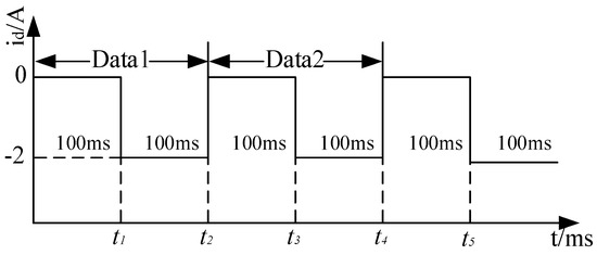
Figure 1. Data sampling chart.

The fourth-order full-rank discrete equation is obtained as:

$$\left\{\begin{array}{l}{u}_{d0}^{\ast ,k}=-{\omega }_{m0}^k{L}_q{i}_{q0}^k-u_{VSI}^k\\ u_{q0}^{\ast ,k}=R_s{i}_{q0}^k+{\omega }_{m0}^k{\psi }_f-u_{VSI}^k\\ u_{d2}^{\ast ,k}=R_s{i}_{d2}^k-{\omega }_{m2}^k{L}_q{i}_{q2}^k-u_{VSI}^k\\ u_{q2}^{\ast ,k}=R_s{i}_{q2}^k+{\omega }_{m2}^k{L}_d{i}_{d2}^k+{\omega }_{m2}^k{\psi }_f-u_{VSI}^k\end{array}\right.$$

(4)

where $k$ is number of iterations, the stator voltage to be compensated is superscripted as “*”, the variable subscripted as “0” is the data sampled with current $i_d=0$, and the variable subscripted as “2” is the data sampled with current $i_d=-2$.

The adjustable model can be designed as:

$$\left\{\begin{array}{l}{u}_{d0}^{\ast ,k}=-{\omega }_{m0}^k{\widehat{L}}_q{i}_{q0}^k-u_{VSI}^k\\ u_{q0}^{\ast ,k}={\widehat{R}}_s{i}_{q0}^k+{\omega }_{m0}^k{\widehat{\psi }}_f-u_{VSI}^k\\ u_{d2}^{\ast ,k}={\widehat{R}}_s{i}_{d2}^k-{\omega }_{m2}^k{\widehat{L}}_q{i}_{q2}^k-u_{VSI}^k\\ u_{q2}^{\ast ,k}={\widehat{R}}_s{i}_{q2}^k+{\omega }_{m2}^k{\widehat{L}}_d{i}_{d2}^k+{\omega }_{m2}^k{\widehat{\psi }}_f-u_{VSI}^k\end{array}\right.$$

(5)

3. Memory Self-Learning GWO

3.1. Grey Wolf Optimization

The GWO emulates the social hierarchy and hunting behavior of grey wolves. The population is structured into four levels: α, β, δ, and ω, in descending order of dominance. The α, β, and δ wolves represent the three best solutions based on fitness evaluation and guide the hunting process, which involves tracking, encircling, and attacking the prey. This mechanism is enhanced by an information feedback system and an adaptively modified convergence factor, which achieves a balance between global exploration and local exploitation. Consequently, the GWO exhibits favorable performance in both convergence speed and accuracy.

In GWO, the lead wolves change position to lead the pack to encircle the prey. The position updating equation is shown as:

$$\left\{\begin{array}{l}\overrightarrow{D}=\left|\overrightarrow{C}\cdot {\overrightarrow{X}}_m(t)-\overrightarrow{X}(t)\right|\\ \overrightarrow{X}(t+1)={\overrightarrow{X}}_m(t)-\overrightarrow{A}\cdot \overrightarrow{D}\end{array}\right.$$

(6)

where $\overrightarrow{D}$ is the distance between grey wolf and prey. ${\overrightarrow{X}}_m$ and $\overrightarrow{X}$ are the position of the prey and the grey wolf, respectively. $t$ is current iteration number. $\overrightarrow{A}$ and $\overrightarrow{C}$ are the coefficient matrices of changes. The following is the calculating formula:

$$\left\{\begin{array}{l}a=2(1-t/M)\\ \overrightarrow{A}=a(2{\overrightarrow{r}}_1-1)\\ \overrightarrow{C}=2{\overrightarrow{r}}_2\end{array}\right.$$

(7)

where ${\overrightarrow{r}}_1$ and ${\overrightarrow{r}}_2$ are two vectors taking values in [0, 1]. t and M are the number of iterations and the maximum number of iterations, respectively. As the number of iterations rises, “a” decreases linearly from 2 to 0. Then the distance between wolves is calculated as follows:

$$\left\{\begin{array}{l}{\overrightarrow{D}}_1=\left|{\overrightarrow{C}}_1\cdot {\overrightarrow{X}}_{\alpha }-\overrightarrow{X}\right|\\ {\overrightarrow{D}}_2=\left|{\overrightarrow{C}}_2\cdot {\overrightarrow{X}}_{\beta }-\overrightarrow{X}\right|\\ {\overrightarrow{D}}_3=\left|{\overrightarrow{C}}_3\cdot {\overrightarrow{X}}_{\delta }-\overrightarrow{X}\right|\end{array}\right.$$

(8)

where ${\overrightarrow{D}}_1$, ${\overrightarrow{D}}_2$, ${\overrightarrow{D}}_3$ are the distances of individual grey wolves from $\alpha$ wolf, $\beta$ wolf, and $\delta$ wolf, respectively. $\overrightarrow{X}$ is the current location of the grey wolf.

Equation (8) indicates the location and orientation of the pack modification. Equation (9) displays the grey wolf’s location that has to be changed. Here the average value is:

$$\left\{\begin{array}{l}{\overrightarrow{X}}_1=\left|{\overrightarrow{X}}_{\alpha }-{\overrightarrow{A}}_1\cdot {\overrightarrow{D}}_1\right|\\ {\overrightarrow{X}}_2=\left|{\overrightarrow{X}}_{\beta }-{\overrightarrow{A}}_2\cdot {\overrightarrow{D}}_2\right|\\ {\overrightarrow{X}}_3=\left|{\overrightarrow{X}}_{\delta }-{\overrightarrow{A}}_3\cdot {\overrightarrow{D}}_3\right|\end{array}\right.$$

(9)

where ${\overrightarrow{X}}_1$, ${\overrightarrow{X}}_2$ and ${\overrightarrow{X}}_3$ indicate the length and direction of the approach to $\alpha$ wolf, $\beta$ wolf, and $\delta$ wolf, respectively. ${\overrightarrow{X}}_{(t+1)}$ represents the grey wolf’s posture that has to be changed.

Figure 2 displays a schematic showing the grey wolf’s updated position:

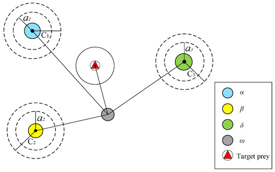
Figure 2. Updated diagram of grey wolves’ location.

The steps of the GWO are:

Step 1: Initialize the grey wolf population.

Step 2: Evaluate the fitness of each wolf and identify the three best wolves as α, β, and δ.

Step 3: Update the coefficient vectors and the position of each wolf using the positions of α, β, and δ.

Step 4: Evaluate the new fitness of each wolf and update the α, β, and δ wolves.

Step 5: Judge whether the termination condition is reached. If the condition is reached, output the α wolf as the optimal solution, and the algorithm run is finished; otherwise, return to step 3 and continue to the next cycle.

3.2. VSI Voltage Compensation

The nonlinearity of the inverter, arising from the saturation voltage drops of the power devices and the voltage drops of the conducting diodes, causes a discrepancy between the actual output voltage and its ideal value. Consequently, this leads to inaccuracies in the identification of motor parameters. The magnitude of these voltage drops is primarily determined by the characteristics of the power devices and the current flowing through them. This issue is particularly pronounced when PMSMs operate in the low-speed zone, where the small reverse electromotive force leads to low voltage, making the inverter’s voltage distortion more significant. In severe cases, it can even challenge stable system operation. Therefore, mitigating the impact of this voltage drop nonlinearity is particularly crucial for the accurate parameter identification of PMSM.

A voltage compensation strategy is advised to reduce the impact and enhance the precision and rate of convergence of parameter identification by lowering output voltage error. The circuit diagram of the three-phase pulse width modulated (PWM) inverter driving the PMSM is depicted in Figure 3.

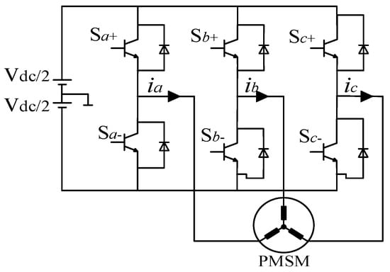
Figure 3. Schematic for a PWM circuit.

The on-state voltage distortion is determined by the conduction of the switching devices and freewheeling diodes and the current direction. Consequently, an analysis of the conduction states across different current paths is required. The current flow paths are categorized into the following four paths; as an example, the current flow paths of the a-phase bridge arm are shown in Figure 4.

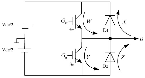
Figure 4. Diagram of a single-phase current route.

The gate signal of a switching tube conducts at different moments with different voltage errors caused by the tube voltage drop. The impact of tube voltage drop on the output voltage is shown in Figure 5, where the switch tube conduction saturation voltage drop is represented by V_CE and the continuity diode voltage drop is represented by V_D.

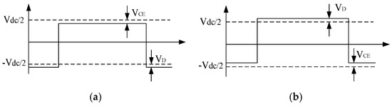
Figure 5. Voltage compensation schematic. (a) $i_x>0$. (b) $i_x<0$.

The direction of the current i_k is defined as the positive direction. When i_k > 0, the gate signal G_m is 1 and S_m turns on. The current path is W in Figure 4. The gate signal G_m is 0, S_m turns off, and D₂ turns on. The current path is Z in Figure 4. When i_k < 0, the gate signal G_n is 1 and S_n turns on. The current path is Y in Figure 4. The gate signal G_n is 0, S_n turns off, and D₁ turns on. The current path is X in Figure 4.

The voltage drops across the inverter switches can be compensated for using Equation (10). This compensation ensures that the actual voltage output to the motor matches the ideal value of the given reference voltage, thereby preventing voltage errors and ensuring safety and stability. With this method, it reduces computational inaccuracies and subsequently enhances identification precision.

$$V_P=\left\{\begin{array}{ll}{\displaystyle \frac{V_{DC}}{2}}-V_{CE}& (\mathrm{path} \mathrm{W})\\ {\displaystyle \frac{V_{DC}}{2}}+V_D& (\mathrm{path} \mathrm{X})\\ -{\displaystyle \frac{V_{DC}}{2}}+V_{CE}& (\mathrm{path} \mathrm{Y})\\ -{\displaystyle \frac{V_{DC}}{2}}-V_D& (\mathrm{path} \mathrm{Z})\end{array}\right.$$

(10)

3.3. Chaotic Reverse Learning GWO (CRLGWO)

The random initialization in GWO often yields populations with poor distribution and diversity, adversely affecting parameter identification accuracy by limiting the search capabilities. To mitigate this, chaotic maps are often incorporated to improve initial population quality and optimality search. However, many maps, including the commonly used logistic map, suffer from non-uniform ergodicity, which directly limits optimization speed and accuracy. To overcome this, we propose initializing the population using the Cat chaotic map integrated with the inverse learning strategy. The Cat map features uniform distribution and fast iteration, given by the following equation:

$$O{P}_k=r_3(X_{\min }^d+X_{\max }^d)-X_k$$

(11)

where $O{P}_k$ is the inverse solution corresponding to $X_k$. $r_3$ is a random number ranging between [0, 1]. $X_{\min }^d$ and $X_{\max }^d$ are the minimum and maximum values of the initial solution in the d dimension, respectively. Some of the poorly adapted solutions in the initial population are excluded in advance through the generation of screen-optimized populations.

The ability of wolves to look for prey both locally and globally is indicated by the value of A in GWO. When $\left|A\right|>1$, grey wolves broaden the boundaries of their hunt and conduct a worldwide search in order to find prey. When $\left|A\right|>1$, the wolves will contract their encirclement and attack the prey, and the grey wolves will conduct localized searches. The magnitude of the convergence factor a determines the value of A. However, in practice, the search process in GWO involves non-linear fluctuations, a dynamic not accurately captured by the linear decrease of the convergence factor a. To better reflect the actual search process, a non-linear cosine-based convergence factor is introduced and defined by the following equation:

$$a_n=\left\{\begin{array}{l}{a}_f+(a_i-a_f){\displaystyle \frac{1+{\left|\cos [(t-1)\pi /(t_{\max }-1)]\right|}^n}{2}},t\le {\displaystyle \frac{t_{\max }}{2}}\\ a_f+(a_i-a_f){\displaystyle \frac{1-{\left|\cos [(t-1)\pi /(t_{\max }-1)]\right|}^n}{2}},{\displaystyle \frac{t_{\max }}{2}}\le t\le t_{\max }\end{array}\right.$$

(12)

where a_n is the cosine convergence factor. a_i and a_f are the initial and final values of a_n, respectively, with a_i = 2 and a_f = 0. t and t_max are the iteration number and maximum iteration number, respectively.

The proposed cosine convergence factor a_n decays slowly in the initial phase, thus promoting global exploration by sustaining a larger A. In the final phase, it decreases rapidly while maintaining a small A to secure effective local exploitation.

3.4. Memory Self-Learning GWO (MSLGWO)

In GWO, the individual’s latest position and the group history optimal solution are considered when α, β and δ wolves command ω wolves for hunting. The α, β, and δ wolves are the group history’s optimal solution for the group, and ω wolves represent the current individual position. However, during the search process, the GWO algorithm mainly exchanges information among the population through the instructions from the superior head wolves to the ω wolves, and then the individual grey wolves update their positions for the search. However, this model overlooks the individual memory of past experiences and the lateral communication among the ω wolves. Inspired by the foraging principle in the PSO, which retains both the global best and personal best positions, we incorporate a similar memory component. The position update equation is as follows:

$$\left\{\begin{array}{l}{v_i}^{k+1}=w{v}_i+c_1{r}_4(P_{best}-x_i)+c_2{r}_5(G_{best}-x_i^k)\\ x_i^{k+1}=x_i^k+v^{k+1}\end{array}\right.$$

(13)

where v_i is particle velocity. x_i is particle position. w is inertia weight. The individual learning factor is denoted by c₁, and the group learning factor by c₂. r₄ and r₅ are random numbers between [0, 1]. P_best and G_best are individual optimal solution and group optimal solution, respectively.

A memory self-learning GWO is proposed combining the idea of individual memory of PSO. The individual experience of the grey wolf is learned, and the influence of the individual optimal position is added to each update of the position. Then the position update formula is as follows:

$${X_i^d}_{(t+1)}=k_1{\displaystyle \sum _{j=\alpha ,\beta ,\delta }{w}_j{X_{i,j}^d}_{(t+1)}+k_2{r}_4(X_{best}^d-{X_i^d}_{(t)})}$$

(14)

where r₄ is a random number of [0, 1]. $X_{best}^d$ is the optimal position of the grey wolf passing through. k₁ and k₂ are constants between [0, 1]. They are the group communication factor and individual memory factor, respectively. The effect of group communication and individual memory of the population on the grey wolf search can be adapted by adjusting the values of k₁ and k₂.

Beyond following the directives from superior wolves, each grey wolf now incorporates its own historical experience into the search process. This mechanism allows individuals to avoid revisiting previously explored positions, thereby preventing redundant evaluations and facilitating a more efficient path toward the optimum. This enhancement directly contributes to improved search accuracy and accelerated convergence speed of the algorithm.

4. Principle of Parameter Identification

By comparing the reference model and the adjustable model based on the fitness function’s magnitude, the concept of parameter identification modifies the adjustable model through the MSLGWO algorithm. The constant reduction of the error between the adjustable model and the reference model ultimately turns into the optimization search issue. The principle of identification is shown in Figure 6.

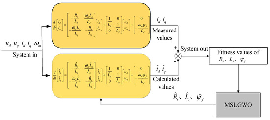
Figure 6. MSLGWO parameter identification schematic.

The control of the motor is actually the control of the two-phase currents, so the fitness function is set according to the currents:

$$\left\{\begin{array}{l}{f}_1={(i_{d0}^k-{\widehat{i}}_{d0}^k)}^2\\ f_2={(i_{q0}^k-{\widehat{i}}_{q0}^k)}^2\\ f_3={(i_{d2}^k-{\widehat{i}}_{d2}^k)}^2\\ f_4={(i_{q2}^k-{\widehat{i}}_{q2}^k)}^2\end{array}\right.$$

(15)

$$C={\displaystyle {\sum }_{i=1}^4{b}_i{f}_i}$$

(16)

where b_i is the weighting factor with a value of 0.25. f_i is the current error squared.

The steps of the MSLGWO are:

Step 1: Acquisition of current, voltage, and angular velocity electrical signals with $i_d=-2$ and $i_d=0$;

Step 2: Cat chaotic mapping with a reverse learning strategy is applied to generate initialized populations.

Step 3: The voltage error due to tube voltage drop nonlinearity is compensated according to Equation (10).

Step 4: Calculate the nonlinear convergence factor a according to Equation (13) and obtain A, C, and D according to Equations (6)–(8).

Step 5: Update the grey wolves’ position according to Equation (15).

Step 6: Calculate fitness values of the wolves and update values of α wolf, β wolf, and δ wolf if the fitness is less than the previous iteration value. If the fitness is greater than the previous iteration value, then return to step 4.

Step 7: When the iteration is completed, the results of the identification of the resistance, inductance, and the flux of the permanent magnet are output.

5. Simulation Analysis

A vector control model of PMSM is constructed in MATLAB/Simulink to examine the recognition impact of the MSLGWO. The control block diagram is displayed in Figure 7. Voltage compensation is added before data acquisition, and then the data sampled will be used as input for the algorithm to obtain the parameters of PMSM, including R, L_s, and ψ_f.

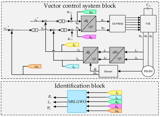
Figure 7. Vector control block diagram of PMSM.

The parameter settings of the PMSM are presented in Table 1.

Table 1. PMSM parameters.

Parameters	Value	Parameters	Value
Pole Pairs	4	ψf	0.167 Wb
R	0.881 Ω	Rated Torque	12 N‧m
Ld	6.72 mH	Rated Speed	1000 rpm
Lq	6.72 mH	Rated Power	1.0 kW

To evaluate and compare the approaches’ identification outcomes, all the initial populations are set to 50, and the boundary values are the same. The simulation running time is 0.3 s, the sampling time is 5 × 10⁻⁶ s, and it is set as the ratio of the running time to the sampling time for the maximum number of iterations. Voltage, current, and electrical angular velocity are sampled. To minimize the accidental error, GWO, GWO_{_vm}, CRLGWO_{_vm}, and MSLGWO_{_vm} were run 10 times under various circumstances, and the mean value was calculated.

(1)

General condition

The torque was set to 12 N∙m and the speed to 1000 r/min, and the algorithms were operated under this working condition. The identified parameters are stator resistance, inductance, and flux. The final average values are derived and recorded in Table 2. The identified values with subscript “vm” take the voltage compensation of inverter tube voltage drop nonlinearity into account, while the identified values without subscript “vm” do not consider the voltage compensation of inverter tube voltage drop nonlinearity.

Table 2. Simulation result of general situation.

Parameters	GWO	GWO_vm	CRLGWO_vm	MSLGWO_vm
R	0.905 Ω	0.898 Ω	0.866 Ω	0.893 Ω
Error	2.724%	1.929%	−1.703%	1.362%
Ls	7.108 mH	6.895 mH	6.554 mH	6.861 mH
Error	5.774%	2.604%	−2.470%	2.098%
ψf	0.175 Wb	0.173 Wb	0.163 Wb	0.170 Wb
Error	4.790%	3.593%	−2.270%	1.796%

(2)

Dynamic condition

Since the motor’s working environment and temperature might have an impact on its properties, after running for a while, the parameters of the motor are shown in Table 3. In a dynamic situation, the torque was increased from 12 N∙m to 16 N∙m in 0.1 s, and the speed was increased from 1000 r/min to 1400 r/min. The parameters recognized under dynamic working conditions are represented in Table 4.

Table 3. New PMSM motor parameter table.

Parameters	Value	Parameters	Value
R	0.890 Ω	ψf	0.162 Wb
Lq	6.640 mH	Ld	6.640 mH

Table 4. Simulation result of general situation.

Parameters	GWO	GWO_vm	CRLGWO_vm	MSLGWO_vm
R	0.935 Ω	0.922 Ω	0.899 Ω	0.897 Ω
Error	5.056%	3.596%	1.011%	0.787%
Ls	6.950 mH	6.843 mH	6.792 mH	6.756 mH
Error	4.669%	3.057%	2.289%	1.747%
ψf	0.167 Wb	0.166 Wb	0.165 Wb	0.164 Wb
Error	3.086%	2.469%	1.852%	1.235%

It is concluded from Table 2 and Table 4 that GWO has a maximum identification error of 5.774% and a minimum of 2.724%. This indicates that GWO suffers from the issues of being easy to fall into local optimum and having poor recognition accuracy. After GWO is compensated for the nonlinearity of the inverter tube voltage drop, the recognition inaccuracy is reduced, the maximum error is 3.596%, and the recognition precision is increased. The recognition accuracy of CRLGWO_{_vm} and MSLGWO_{_vm} based on tube voltage drop compensation is better than that of GWO. The MSLGWO_{_vm} error is limited to 2.098%, featuring high recognition accuracy and robustness.

6. Experimental Verification

6.1. Discussion on Validation

The viability of the suggested methodology is confirmed using the RT-LAB hardware-in-the-loop simulation (HILS) experimental platform, as depicted in Figure 8. The platform contains an RT-LAB simulator, DSP controller, motor drive model constructed in RT-LAB with a host computer and an oscilloscope. The TMS320F2812 DSP controller implements the proposed identification algorithm. The host computer conducts continuous data collection. Waveform recording and validation are accomplished using an oscilloscope.

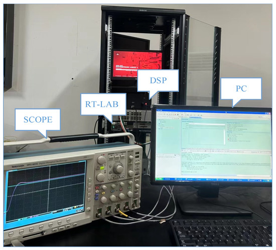
Figure 8. Diagram of experimental apparatus.

The HIL experiment platform is simulated by connecting some of the physical parts in the simulation system and testing the physical part by constructing the simulation model of the system to obtain the similar effect as the full physical experiment. It demonstrates distinct advantages over both physical motor testing and pure digital simulation for motor parameter identification. The physical testing faces inherent limitations, including fixed parameters and unknown actual operational parameters, while RT-LAB simulation enables precise determination of operational parameters, provides sufficient dynamic response for capturing transient characteristics, and maintains credible verification through real-time signal processing. This configuration combines the flexibility of simulation with the reliability of physical experiments, providing a more robust and convincing platform for verification under various operating conditions.

6.2. Experimental Results

(1)

General condition

The speed is 1000 r/min, and the torque is 12 N/m. The GWO, GWO_{_vm}, CRLGWO_{_vm}, and MSLGWO_{_vm} are used to recognize the motor parameters at general condition. The resistance identification curve under this operating state is presented in Figure 9, the inductance identification curve is shown in Figure 10, and the permanent magnet flux identification curve is shown in Figure 11.

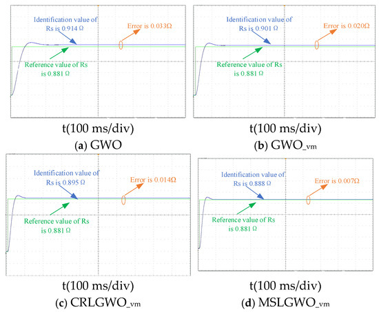
Figure 9. Resistance identification curves of general condition.

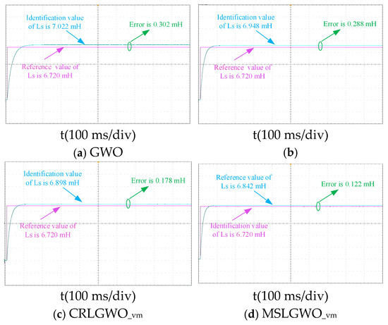
Figure 10. Inductive identification curves in general condition.

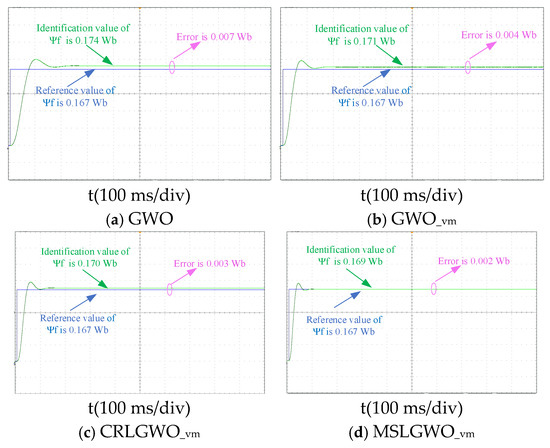
Figure 11. Permanent magnet flux identification curves in general condition.

Under general conditions, as can be seen in Figure 9, the convergence times of GWO, GWO_{_vm}, CRLGWO_{_vm}, and MSLGWO_{_vm} are 0.2 s, 0.15 s, 0.1 s, and 0.08 s, respectively. The GWO’s convergence speed is effectively accelerated after considering the inverter tube voltage drop nonlinearities.

As can be seen in Figure 10, the recognition errors of GWO, GWO_{_vm}, CRLGWO_{_vm}, and MSLGWO_{_vm} are 4.50%, 3.39%, 2.65%, and 1.81%. The algorithms that conducted the tube dropout voltage compensation all reduced the discrimination errors, with MSLGWO_{_vm} having the highest accuracy.

As can be seen from Figure 11, compared to GWO, GWO_{_vm}, CRLGWO_{_vm}, and MSLGWO_{_vm} recognize faster as well as overshoot less. The convergence time is 0.21 s, and the GWO recognition error is 4.192%. With a convergence time of only 0.09 s, the MSLGWO_{_vm} recognition error is 1.198%.

Table 5 presents the recognized mean values of the experiments under general conditions.

Table 5. Experiment result for general situation.

Parameters	GWO	GWO_vm	CRLGWO_vm	MSLGWO_vm
R	0.914 Ω	0.901 Ω	0.895 Ω	0.888 Ω
Error	3.746%	2.270%	1.589%	0.795%
Ls	7.022 mH	6.948 mH	6.898 mH	6.842 mH
Error	4.494%	3.393%	2.649%	1.815%
ψf	0.174 Wb	0.171 Wb	0.170 Wb	0.169 Wb
Error	4.192%	2.395%	1.796%	1.198%

It can be concluded from the data provided in Table 5 that the maximum identification error for the GWO algorithm is 4.494%, whereas for the algorithm considering compensation of the inverter’s nonlinear voltage drops, it does not exceed 3.393%. This substantiates that the identification accuracy is improved after incorporating voltage compensation. MSLGWO_{_vm} achieves a maximum error of no more than 1.198% and exhibits the fastest convergence speed. It can be seen that the accuracy of the algorithm is improved after compensating for the inverter tube voltage drop nonlinearity, and after taking into account the grey wolf’s individual experience with reverse learning, the algorithm’s capacity for both local and global seeking is strengthened, and its identification speed and accuracy are further improved.

(2)

Dynamic condition

The experiments are operated under dynamic working conditions with variable parameters, and the GWO, GWO_{_vm}, CRLGWO_{_vm}, and MSLGWO_{_vm} algorithms are implemented to identify the motor parameters. Under the dynamic condition, the resistance identification curve is presented in Figure 12, the inductance identification curve is presented in Figure 13, and the permanent magnet flux identification curve is presented in Figure 14. The results of the four methods running under dynamic conditions are shown in Table 6.

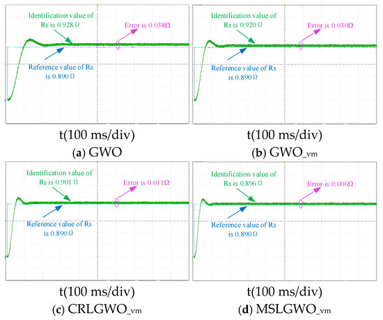
Figure 12. Resistance identification curves in dynamic condition.

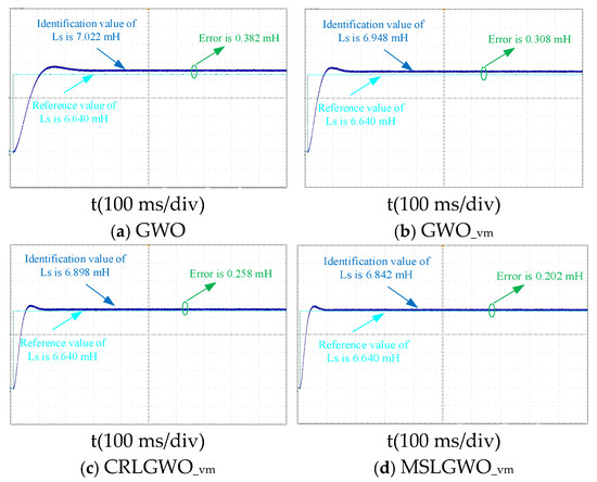
Figure 13. Inductive identification curves in dynamic condition.

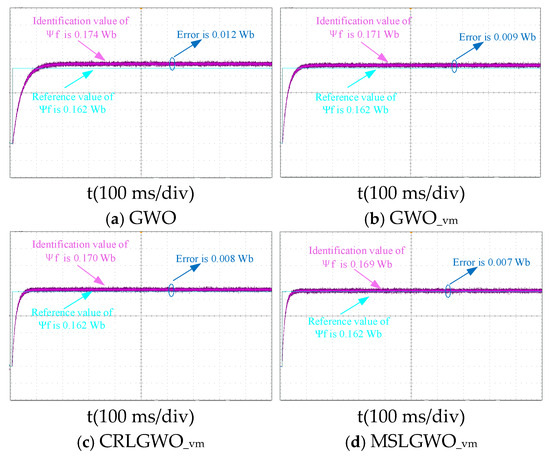
Figure 14. Permanent magnet flux identification curves in dynamic condition.

Table 6. Experiment result for dynamic situation.

Parameters	GWO	GWO_vm	CRLGWO_vm	MSLGWO_vm
R	0.928Ω	0.920Ω	0.901Ω	0.896Ω
Error	4.270%	3.371%	1.236%	0.674%
Ls	7.114 mH	6.987 mH	6.910 mH	6.830 mH
Error	7.139%	5.226%	4.066%	2.861%
ψf	0.176 Wb	0.173 Wb	0.171 Wb	0.169 Wb
Error	8.642%	6.790%	5.556%	4.321%

As can be seen in Figure 12, the resistance recognition curve fluctuates under dynamic working conditions. The identification error of GWO increases by 0.46%, and GWO_{_vm} increases by 0.97% compared to the general working condition. While the identification errors of CRLGWO_{_vm} and MSLGWO_{_vm} decreased by 0.41% and 0.18%, respectively. Therefore, the recognition error of MSLGWO_{_vm} is only 0.67% under dynamic working conditions, and it has a better performance against interference.

As can be seen in Figure 13, the recognition times of GWO, GWO_{_vm}, CRLGWO_{_vm}, and MSLGWO_{_vm} are affected differently in dynamic working conditions compared to the general working conditions, which are 0.25 s, 0.15 s, 0.1 s, and 0.08 s, respectively. The recognition times of GWO and GWO_{_vm} are lengthened by 0.1 s and 0.03 s, respectively, and the recognition times of CRLGWO_{_vm} and MSLGWO_{_vm} both shorten the recognition time by 0.02 s. These results reflect that MSLGWO_{_vm} has a fast response time and is suitable for areas where fastness is required.

As shown in Figure 14, under dynamic operating conditions, the maximum identification error is reduced to 6.790% with voltage compensation, compared to 8.642% without compensation. Further improvements are observed with the CRLGWO_{_vm} and MSLGWO__vm, achieving maximum errors of 5.556% and 4.321%, respectively. These results demonstrate the superior identification accuracy of the proposed MSLGWO_{_vm} in a dynamic condition.

Table 6 displays the outcomes of the experimental runs of the four approaches conducted under dynamic operating settings.

According to the results in Table 6, the error of GWO algorithm identification is reduced by at least 21.0% after compensating for the nonlinearity of the inverter tube voltage drop. CRLGWO_{_vm} and MSLGWO_{_vm} decreased by at least 35.7% and 50.0%, respectively. Among them, MSLGWO_{_vm} shows the highest accuracy.

7. Conclusions

To address the issues of voltage distortion from VSI causing errors in PMSM parameter identification, as well as the poor accuracy and slow late-stage convergence of the traditional GWO, an MSLGWO parameter identification method with voltage error compensation is proposed. This method compensates for the inverter’s nonlinear voltage drops, thereby improving identification accuracy and reducing voltage errors. The following conclusions are drawn based on experimental data and theoretical analysis. The following conclusions are reached based on the experimental data and theoretical reasoning.

(1)

By accounting for the impact of inverter nonlinear voltage drops on PMSM parameter identification and compensating for the resulting voltage error, the algorithm’s identification accuracy is significantly improved. Compared with the experimental conditions of uncompensated voltage, the identification error is significantly reduced by at least 24.5% under general working conditions and by at least 20.0% under dynamic working conditions.

(2)

The initial population’s variety is guaranteed by the combination of the reverse learning strategy with Cat chaotic mapping. The range of the search is widened. A cosine-varying nonlinear convergence factor is introduced, balancing the global search capability and local search capability, and the speed of optimization search is improved. Compared with GWO, the identification times for resistance, inductance, and magnetic flux are reduced by 0.1 s, 0.03 s, and 0.06 s for general working condition and by 0.13 s, 0.15 s, and 0.13 s for dynamic working condition, respectively.

(3)

Memory learning of individual experiences of grey wolves and enhanced group information exchange during search introduces the influence of individual optimal positions when updating positions. The method enhances the speed and accuracy of the search. Considering the inverter tube voltage drop nonlinearity, the maximum error of GWO is 3.393% for general working condition and 1.815% for MSLGWO, and the identification time is within 0.1 s. The maximum error of GWO is 6.790%, and that of MSLGWO is 4.321% under dynamic working conditions, and the recognition time is less than 0.11 s. The experimental results confirm that the MSLGWO_{_vm} possesses superior identification accuracy, faster convergence speed, and satisfactory dynamic performance.

References

- Sun, L.; Li, X.; Chen, L. Motor Speed Control with Convex Optimization-Based Position Estimation in the Current Loop. IEEE Trans. Power Electron. 2021, 36, 10906–10919. [Google Scholar] [CrossRef]
- Wang, Q.; Zhao, X.; Yang, P.; Hua, W.; Buja, G. Effects of Triangular Wave Injection and Current Differential Terms on Multiparameter Identification for PMSM. IEEE Trans. Power Electron. 2023, 39, 2943–2947. [Google Scholar] [CrossRef]
- Wang, Z.; Chai, J.; Xiang, X.; Sun, X.; Lu, H. A Novel Online Parameter Identification Algorithm Designed for Deadbeat Current Control of the Permanent-Magnet Synchronous Motor. IEEE Trans. Ind. Appl. 2021, 58, 2029–2041. [Google Scholar] [CrossRef]
- Liu, S.; Wang, Q.; Zhang, G.; Wang, G.; Xu, D. Online Temperature Identification Strategy for Position Sensorless PMSM Drives with Position Error Adaptive Compensation. IEEE Trans. Power Electron. 2022, 37, 8502–8512. [Google Scholar] [CrossRef]
- Liu, X.; Du, Y. Torque Control of Interior Permanent Magnet Synchronous Motor Based on Online Parameter Identification Using Sinusoidal Current Injection. IEEE Access 2022, 10, 40517–40524. [Google Scholar] [CrossRef]
- Wang, Q.; Wang, G.; Zhao, N.; Zhang, G.; Cui, Q.; Xu, D. An Impedance Model-Based Multiparameter Identification Method of PMSM for Both Offline and Online Conditions. IEEE Trans. Power Electron. 2021, 36, 727–738. [Google Scholar] [CrossRef]
- Wallscheid, O.; Bocker, J. Global Identification of a Low-Order Lumped-Parameter Thermal Network for Permanent Magnet Synchronous Motors. IEEE Trans. Energy Convers. 2016, 31, 354–365. [Google Scholar] [CrossRef]
- Liu, Z.; Feng, G.; Han, Y. Extended-Kalman-Filter-Based Magnet Flux Linkage and Inductance Estimation for PMSM Considering Magnetic Saturation. In Proceedings of the 36th Youth Academic Annual Conference of Chinese Association of Automation (YAC), Nanchang, China, 28–30 May 2021. [Google Scholar]
- Shi, S.; Guo, L.; Chang, Z.; Zhao, C.; Chen, P. Current Controller Based on Active Disturbance Rejection Control with Parameter Identification for PMSM Servo Systems. IEEE Access 2023, 11, 46882–46891. [Google Scholar] [CrossRef]
- Xu, W.; Tang, Y.; Dong, D.; Xiao, X.; Liu, Y.; Yang, K.; Li, Y. Improved Deadbeat Predictive Thrust Control for Linear Induction Machine with Online Parameter Identification Based on MRAS and Linear Extended State Observer. IEEE Trans. Ind. Appl. 2023, 59, 3186–3199. [Google Scholar] [CrossRef]
- Brosch, A.; Hanke, S.; Wallscheid, O.; Bocker, J. Data-Driven Recursive Least Squares Estimation for Model Predictive Current Control of Permanent Magnet Synchronous Motors. IEEE Trans. Power Electron. 2021, 36, 2179–2190. [Google Scholar] [CrossRef]
- Li, X.; Kennel, R. General Formulation of Kalman-Filter-Based Online Parameter Identification Methods for VSI-Fed PMSM. IEEE Trans. Ind. Electron. 2021, 68, 2856–2864. [Google Scholar] [CrossRef]
- Su, G.; Wang, P.; Guo, Y.; Cheng, G.; Wang, S.; Zhao, D. Multiparameter Identification of Permanent Magnet Synchronous Motor Based on Model Reference Adaptive System—Simulated Annealing Particle Swarm Optimization Algorithm. Electronics 2022, 11, 159. [Google Scholar] [CrossRef]
- Zhou, S.; Wang, D.; Li, Y. Parameter Identification of Permanent Magnet Synchronous Motor Based on Modified- Fuzzy Particle Swarm Optimization. Energy Rep. 2022, 9, 873–879. [Google Scholar] [CrossRef]
- Ahandani, M.A.; Abbasfam, J.; Kharrati, H. Parameter Identification of Permanent Magnet Synchronous Motors Using Quasi-Opposition-Based Particle Swarm Optimization and Hybrid Chaotic Particle Swarm Optimization Algorithms. Appl. Intell. 2022, 52, 13082–13096. [Google Scholar] [CrossRef]
- Wang, Z.; Yang, M.; Gao, L.; Wang, Z.; Zhang, G.; Wang, H.; Gu, X. Deadbeat Predictive Current Control of Permanent Magnet Synchronous Motor Based on Variable Step-Size Adaline Neural Network Parameter Identification. IET Electr. Power Appl. 2020, 14, 2007–2015. [Google Scholar] [CrossRef]
- Yang, J.; Shen, Y.; Tan, Y. Parameter Compensation for the Predictive Control System of a Permanent Magnet Synchronous Motor Based on Bacterial Foraging Optimization Algorithm. World Electr. Veh. J. 2024, 15, 23. [Google Scholar] [CrossRef]
- Peesapati, R.; Kumar, N. Electricity Price Forecasting and Classification through Wavelet–Dynamic Weighted PSO–FFNN Approach. IEEE Syst. J. 2018, 12, 3075–3084. [Google Scholar]
- Chawla, V.K.; Chanda, A.K.; Angra, S. Multi-Load AGVs Scheduling by Application of Modified Memetic Particle Swarm Optimization Algorithm. J. Braz. Soc. Mech. Sci. Eng. 2018, 40, 436. [Google Scholar] [CrossRef]
- Xu, W.; Ismail, M.M.; Liu, Y.; Islam, M.R. Parameter Optimization of Adaptive Flux-Weakening Strategy for Permanent-Magnet Synchronous Motor Drives Based on Particle Swarm Algorithm. IEEE Trans. Power Electron. 2019, 34, 12128–12140. [Google Scholar] [CrossRef]
- Sun, X.; Zhang, Y.; Tian, X.; Cao, J.; Zhu, J. Speed Sensorless Control for IPMSMs Using a Modified MRAS with Gray Wolf Optimization Algorithm. IEEE Trans. Transp. Electrif. 2022, 8, 1326–1337. [Google Scholar] [CrossRef]
- Hou, Y.; Gao, H.; Wang, Z.; Du, C. Improved Grey Wolf Optimization Algorithm and Application. Sensors 2022, 22, 3810. [Google Scholar] [CrossRef]
- Jiang, J.; Zhang, Z. Multi-Parameter Identification of Permanent Magnet Synchronous Motor Based on Improved Grey Wolf Optimization Algorithm. In Proceedings of the 2021 IEEE 4th Student Conference on Electric Machines and Systems (SCEMS), Huzhou, China, 1–3 December 2021. [Google Scholar]
- Liu, H.; Cao, L. Parameter Identification of Generator Excitation System Based on Improved Grey Wolf Optimization. J. Phys. Conf. Ser. 2020, 1626, 012009. [Google Scholar] [CrossRef]
- Chen, Z.; Yu, Y.; Wang, Y. Parameter Identification of Jiles-Atherton Model Based on Levy Whale Optimization Algorithm. IEEE Access 2022, 10, 66711–66721. [Google Scholar] [CrossRef]
- Zhu, J.; Zhu, W.; Zhi, P.; Wei, H. Design of a PMSM Speed Regulation System Based on an Improved GWO Algorithm. In Proceedings of the IEEE International Conference on Mechatronics and Automation (ICMA), Harbin, China, 6–9 August 2023. [Google Scholar]
- Djerioui, A.; Houari, A.; Machmoum, M.; Ghanes, M. Grey Wolf Optimizer Based Predictive Torque Control for Electric Vehicle Applications. In Proceedings of the 22nd European Conference on Power Electronics and Applications (EPE’20 ECCE Europe), Lyon, France, 7–11 September 2020. [Google Scholar]
- Yu, X.; Jiang, N.; Wang, X.; Li, M. A Hybrid Algorithm Based on Grey Wolf Optimizer and Differential Evolution for UAV Path Planning. Expert Syst. Appl. 2023, 215, 119327. [Google Scholar] [CrossRef]
- Wang, Z.; Lin, M.; Chen, D. A New Grey Wolf Optimization Algorithm with Improved Convergence Factor and Mutation Strategy. In Proceedings of the 35th Youth Academic Annual Conference of Chinese Association of Automation (YAC), Zhanjiang, China, 16–18 October 2020. [Google Scholar]
- Fang, H.; Zha, S. Flux Modulated Permanent Magnet Generator Optimization with Improved Gray Wolf Algorithm. In Proceedings of the 2022 25th International Conference on Electrical Machines and Systems (ICEMS), Chiang Mai, Thailand, 29 November–2 December 2022. [Google Scholar]
- Lee, J.; Seo, H.; Lee, J.-S.; Han, B.-K.; Mok, H.-S. Electrical Parameter Estimation Method for Surface-Mounted Permanent Magnet Synchronous Motors Considering Voltage Source Inverter Nonlinearity. IEEE Access 2023, 11, 16288–16296. [Google Scholar] [CrossRef]
- Lu, G.; Su, J.; Yang, G.; Liu, F. Offline Parameter Self-Learning Method for Low-Impedance Dual Three-Phase PMSMs: Addressing AC Losses and Inverter Nonlinearity. IEEE J. Emerg. Sel. Top. Power Electron. 2024, 12, 2730–2743. [Google Scholar] [CrossRef]
- Chen, D.; Wang, J.; Zhou, L. Adaptive Second-Order Active-Flux Observer for Sensorless Control of PMSMs with MRAS-Based vsi Nonlinearity Compensation. IEEE J. Emerg. Sel. Top. Power Electron. 2023, 11, 3076–3086. [Google Scholar] [CrossRef]
- Wang, Q.; Liu, S.; Zhang, G.; Ding, D.; Li, B.; Wang, G.; Xu, D. Zero-Sequence Voltage Error Elimination-Based Offline vsi Nonlinearity Identification for PMSM Drives. IEEE Trans. Transp. Electrif. 2024, 10, 55–66. [Google Scholar] [CrossRef]
- Liu, Z.-H.; Wei, H.-L.; Li, X.-H.; Liu, K.; Zhong, Q.-C. Global Identification of Electrical and Mechanical Parameters in PMSM Drive Based on Dynamic Self-Learning PSO. IEEE Trans. Power Electron. 2018, 33, 10858–10871. [Google Scholar] [CrossRef]
Disclaimer/Publisher’s Note: The statements, opinions and data contained in all publications are solely those of the individual author(s) and contributor(s) and not of MDPI and/or the editor(s). MDPI and/or the editor(s) disclaim responsibility for any injury to people or property resulting from any ideas, methods, instructions or products referred to in the content. |
© 2025 by the authors. Licensee MDPI, Basel, Switzerland. This article is an open access article distributed under the terms and conditions of the Creative Commons Attribution (CC BY) license (https://creativecommons.org/licenses/by/4.0/).