Abstract
Current denoising algorithms in infrared imaging systems predominantly target either high-frequency stripe noise or Gaussian noise independently, failing to adequately address the prevalent hybrid noise in real-world scenarios. To tackle this challenge, we propose a convolutional neural network (CNN)-based approach with a refined composite loss function, specifically designed for hybrid noise removal in raw infrared images. Our method employs a residual network backbone integrated with an adaptive weighting mechanism and edge-preserving loss, enabling joint modeling of multiple noise types while safeguarding structural edges. Unlike reference-based CNN denoising methods requiring clean images, our solution leverages intrinsic gradient variations within image sequences for adaptive smoothing, eliminating dependency on ground-truth data during training. Rigorous experiments conducted on three public datasets have demonstrated the optimal or suboptimal performance of our method in mixed noise suppression and detail preservation (PSNR > 32.13/SSIM > 0.8363).
1. Introduction
Infrared cameras exhibit significant penetration advantages in complex environments such as haze, rain, snow, and nighttime, rendering them indispensable for industrial inspection, security surveillance, autonomous driving, and medical diagnostics [1,2,3,4]. However, uncooled infrared cameras suffer from the temporal response drift of pixels due to material properties, while environmental temperature variations introduce noise that typically manifests as vertical stripe artifacts with superimposed random noise components [5]. Such hybrid noise not only degrades visual quality but also renders conventional single-point calibration-based non-uniformity correction ineffective, causing residual noise to be amplified during enhancement algorithms [6,7,8]. In computer vision, denoising techniques have achieved remarkable progress. Pixel-domain and frequency-domain approaches represent two predominant paradigms: the former directly manipulates image matrices through methods like wavelet transforms and guided filtering [9], whereas the latter employs mathematical transformations to frequency representations for noise suppression [10].
In recent years, breakthroughs in deep learning have continuously pushed the boundaries of image denoising performance, with convolutional neural networks (CNNs) emerging as the most prominent approach [11,12,13]. Nevertheless, existing methods predominantly focus on addressing either stripe noise or speckle noise individually, often employing complex network architectures that pose challenges for hardware deployment. Most state-of-the-art denoising algorithms specialize in either random noise or stripe noise suppression, whereas real-world scenarios typically involve hybrid noise patterns [14,15]. Stripe-oriented methods frequently compromise image texture fidelity while leaving residual random noise amplified [15]. Conversely, random-noise-targeted approaches exhibit excessive sensitivity to textural structures, tending to preserve or even accentuate stripe artifacts during smoothing operations. Ding et al. pioneered SNRCNN for stripe noise reduction, though its efficacy markedly deteriorates when encountering amplified random noise [16,17]. Chang et al. achieved superior denoising through residual networks incorporating long-short-term learning strategies [18]. Beyond CNN frameworks, U-Net’s encoder–decoder architecture has demonstrated exceptional denoising capabilities. Kuang’s team further developed DDLSR for stripe noise elimination [19], while Yuan et al. proposed AscNet to address inter-layer semantic gaps and inadequate global column feature representation, setting new benchmarks in stripe removal [20].
The approach targeting random noise has gained renewed vitality with the advancement of deep learning. Zhang et al. proposed DnCNN, which pioneered the application of deep CNNs to image denoising through residual learning and batch normalization, demonstrating the superiority of end-to-end models in Gaussian noise scenarios [21]. Architecturally, DruNet combined U-Net framework with residual blocks to enhance global-local information fusion, redefining the state-of-the-art denoising benchmarks [22]. Shen et al. further improved performance by integrating transpose attention modules into symmetric encoder–decoder structures [23]. Despite the flourishing development of deep learning, most methods focus solely on architectural innovations. Although achieving remarkable results, they lack differentiated processing for hybrid noise and fail to meet hardware deployment requirements [12]. This study proposes an improved loss function based on lightweight architecture, leveraging gradient variation characteristics of FPN stripes to guide edge-stripe discrimination. The solution enables precise convergence with compact networks, providing a practical scheme for future researchers to simplify architectures and facilitate hardware deployment.
Overall, the contributions of this work are threefold:
- A self-supervised localization strategy combining Gaussian-blurred references with gradient-variance analysis to decouple stripe-random noise mixtures without clean-image supervision.
- An adaptive TV-regularization framework with spatially variant weight assignment, achieving texture-aware smoothing while preserving structural edges.
- A lightweight edge-preserving module integrated into the denoising pipeline, enabling simultaneous noise suppression and high-frequency detail retention for hardware-efficient deployment.
2. Related Work
2.1. Mixed Noise Modeling Using Prior Knowledge
In traditional mixed noise removal methods, regularization constraints are primarily constructed based on prior knowledge to model stripe noise and image components. Kang et al. employed a unidirectional regularization term and non-convex group sparsity term to capture stripe structures, while applying non-convex fractional total variation (FTV) regularization to image components. This approach mitigated the “staircase effect” commonly induced by conventional total variation (TV) models, enabling effective stripe extraction and smooth denoising under strong noise interference. Chen et al. leveraged the group sparsity property of stripe noise combined with unidirectional TV regularization for noise modeling, alongside standard TV regularization for image smoothing, achieving joint removal of mixed noise in remote sensing images [24]. Yang et al. characterized stripe noise as a low-rank matrix by exploiting its low-rank property, integrating unidirectional hybrid TV to preserve details and structures in other directions during denoising [25]. Furthermore, Chen et al. proposed a unified framework combining unidirectional TV constraints with wavelet-based sparse regularization, enabling simultaneous recovery of destriped images and separated noise from a single input image [26].
2.2. Modeling Mixed Noise Using Neural Networks
With the advancement of deep learning, neural network-based denoising for complex infrared images has achieved remarkable progress. Hu et al. proposed an end-to-end deep learning network with a symmetric multi-scale encoder–decoder sampling structure, which extracts and fuses multi-scale information from different depth levels of the network to better simulate the complex scenarios of mixed noise sources in real-world applications [27]. Addressing the simultaneous presence of fixed pattern noise (FPN) and blur artifacts in infrared images, Lee et al. developed a unified algorithmic framework. This framework first establishes an infrared linear degradation model to accurately estimate FPN, then combines the unique gradient statistical characteristics of infrared images for non-blind deconvolution, achieving significant processing results [28]. Pan et al. adopted a sequential multi-task learning framework, decomposing the complex destriping task into three auxiliary subtasks, and proposed a model named Stripe Location-Dependent Restoration Network (SLDR), which achieved precise destriping and high-quality image restoration [29]. For specific mixed noise in infrared images, Wang et al. designed a dual-encoder denoising network based on U-Net architecture, where two parallel encoder branches perform noise perception and encoding at different receptive fields to reconstruct high-quality infrared images [30]. Huang et al. introduced dual auxiliary variables, combining residual CNN and U-shaped networks to alternately model stripe noise and random noise, enabling efficient separation and removal of mixed noise [31].
3. Proposed Method
In Section 3.1, the denoising workflow of the proposed algorithm is briefly described; in Section 3.2, the training methodology for this optimization model is detailed; and Section 3.3 presents in full the compound loss function employed to guide the network’s self-supervised training.
3.1. Denoising Method
Deep learning with attention mechanisms has been extensively applied to image denoising tasks in recent years [21,22,23]. In contrast, the proposed method aims to achieve effective noise removal using a lightweight convolutional neural network (CNN). As illustrated in Figure 1, the approach takes a noisy image as input, predicts a pixel-wise noise estimation map via a trained CNN, and ultimately reconstructs the corresponding clean image through a residual subtraction operation.
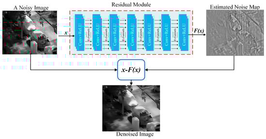
Figure 1.
Denoising workflow of the proposed method.
3.2. Model Training Methodology
Figure 2 illustrates the self-supervised training pipeline of the proposed method. The framework takes a set of noisy infrared images as input. To address the scarcity of clean images in real-world scenarios, a surrogate supervision signal—generated by applying Gaussian blurring or degradation operations to noisy images—is introduced during training. The primary objective of this loss component is to achieve pixel-level localization of mixed noise. Furthermore, the loss function incorporates a gradient and variational regularization term weighted by edge detection, designed to suppress noise in flat regions while effectively preserving edge information. Ultimately, through joint optimization of these three loss functions, the network enhances its capability to model fixed-pattern noise in infrared imagery under constrained parameter budgets.
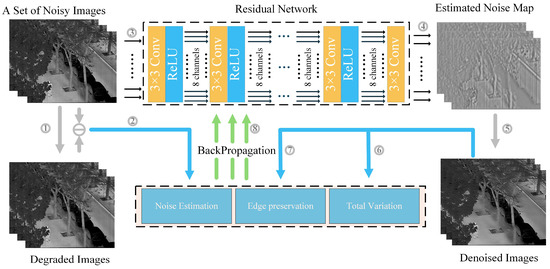
Figure 2.
The multi-scale guidance and adaptive edge perception training process of the proposed method. The quantity and process of training are numbered in the figure.
In mixed-noise removal tasks, prior studies have identified offset components as one of the primary sources of noise [32]. Consequently, in the proposed method, noise is modeled as the non-uniform gain and bias of each pixel in a clean image, mathematically represented by the following “gain-bias” formula:
where I denotes the noisy image, C represents the ideal image, P is the pixel wise gain matrix, B is the pixel wise bias matrix, and both are approximately invariant in time, together forming the FPN mode. “⊙” represents element-wise multiplication operation. Nt is a random noise that varies over time, assuming it has zero mean and follows a heteroscedasticity distribution.
For the convenience of subsequent description, Equation (1) will be simplified as follows:
where represents the fixed noise caused by pixel-by-pixel gain-bias, which can be expressed by the following formula:
Therefore, when the network learns the noise patterns in consecutive frames, it can obtain the ideal image through additive operations:
where is the noise pattern map estimated by the network for the input image, and is the output of the ideal image. Based on the above model, and utilizing the powerful region perception ability of convolutional neural networks (CNN), by distinguishing between edges and noise, it is possible to effectively predict the noise pattern of each frame of the image and obtain the ideal image.
3.3. Loss Term Design
3.3.1. Noise Estimation Term
Fixed-pattern noise in identical cameras manifests as positionally invariant striping artifacts, as shown in Figure 3. To leverage this characteristic, a differential supervision term based on degraded observations is incorporated into the loss function:
where denotes the L2-norm constrained noise estimation loss term, represents the difference between the input image and degraded image, and signifies the noise pattern predicted by the network.
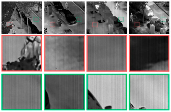
Figure 3.
Amplified visualization shows the fixed characteristics of mixed noise patterns across spatial regions under multi frame conditions. The red and green borders represent different areas in the original graphic marker.
3.3.2. Edge Preservation with TV Regularization
In image denoising, variational regularization is often used to suppress gradient variations and reduce noise. However, classical total variation (TV) models struggle to distinguish between texture and noise, especially in infrared images where fixed-pattern noise (FPN) can mimic authentic textures. This limitation can lead to structural blurring, which is problematic in conventional denoising methods. To overcome this challenge, we propose an enhanced TV regularizer that adaptively adjusts the smoothing penalty across regions using a gradient-aware exponential weighting mechanism. This approach enables more effective noise suppression in flat areas while preserving texture and edge details. The edge weight map is computed as follows:
where θ denotes a hyperparameter iteratively adapted during training to modulate the effective range of gradient influence. represents the local image gradient in horizontal and vertical directions. The computational formulation of θ is given below:
where and modulate the mean and variance of the gradient matrix , respectively, and represents an adjustable parameter. is defined as follows:
Edge regions typically exhibit elevated gradient magnitudes. Constructing weights based on gradient information effectively preserves edge details while preventing edge blurring caused by excessive smoothing. The calculation process of adaptive gradient perception weights is shown in Figure 4.
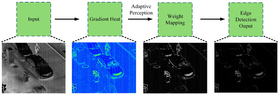
Figure 4.
Display the processing procedure of the adaptive edge perception module. To demonstrate its effectiveness in the actual training process, this is a noisy infrared image.
This weighting mechanism enhances adaptability to multimodal noise patterns by integrating local gradient characteristics with denoising strength. Consequently, it improves overall output quality and redirects noise estimation processes away from edges. Figure 4 demonstrates the method’s effectiveness across sequential frames.
The upper section of Figure 5 displays pseudo clean images, while the lower section of Figure 5 presents weight maps generated by the edge detection mechanism.
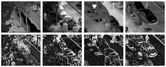
Figure 5.
The effect of applying our adaptive edge detection algorithm in different scenarios on the LLVIP dataset. To achieve the best observation effect, this is a set of clean images.
Building upon the aforementioned edge-weighting factors, we present the final improved TV regularization term as follows:
where “∘” denotes the element-wise multiplication operation. This design effectively attenuates smoothing intensity in edge regions, thereby preventing structural damage to image edges.
utilizes edge detection weights to suppress smoothing in edge regions, thereby preventing direct structural damage to edges. However, it may still induce local distortion near edges. To enhance edge preservation capability, our proposed framework incorporates an L1-norm loss term () to optimize edge retention performance. By computing the absolute difference between denoised results and pristine ground-truth images, this L1 loss drives the network to better learn edge detail preservation during training. The formal definition is as follows:
This loss term further ensures the network’s feature retention capability in edge regions.
In summary, the total loss function proposed in this paper consists of a weighted combination of the following three terms, where and are the weighting coefficients for each loss component. The specific values of these coefficients will be elaborated in the experimental section.
4. Experiments
4.1. Experimental Design
In order to verify the effectiveness of the proposed method, multiple datasets were used for training and testing in the experiment, including LLVIP, CVC09, DLS-NUC, and self-collected images for training and evaluation. Due to the large size of the LLVIP and CVC09 datasets, a sequence-based (scene ID) partitioning method (seed = 1234) is used to ensure that the same scene does not appear in different subsets and cause leakage.
- (1)
- LLVIP (subset): Uniform random sampling is performed from all sequences, using only the infrared modality. A total of 300 images are obtained for training, and 200 are obtained for testing. The same sequence only appears in one subset. After partitioning, we perform near duplicate checks across subsets: if the SSIM of two images is ≥0.95, we remove the test side image to eliminate potential leaks.
- (2)
- CVC09/DLS-NUC/Self Captured Set: Used as an external test set, each containing 100/100/100 images. Not participating in training.
- (3)
- Preprocessing and Sampling: During the training phase, the image is uniformly scaled to 256 × 256 and only 256 × 256 non-overlapping patches are extracted from the original training image. During the verification/testing phase, the entire image is evaluated, patches do not cross subsets, and data augmentation is not performed on the test set.
- (4)
- Synthetic noise evaluation (optional): To analyze the robustness of the model to stripe and Gaussian components, we only use stripe-Gaussian noise data augmentation during the training phase. We construct another synthetic test set for additional analysis. The real test sets do not add additional noise.
For publicly available datasets providing reference images, peak signal-to-noise ratio (PSNR) and structural similarity index (SSIM) are adopted as objective evaluation metrics to quantify denoising effectiveness.
All experiments were conducted on synthetically corrupted images. Clean images were superimposed with two types of noise: Gaussian stripe noise with varying standard deviations and random noise. The overall noise intensity was defined as . To enhance model robustness, each image was randomly cropped into 256 × 256 pixel patches during training. These patches were fed into the network in mini-batches of 16 images per batch, with random flipping applied for data augmentation.
In the proposed method, the weight set remains fixed during training with assigned values of . The Adam optimizer is employed with default parameter settings. The maximum number of iterations is set to 50 epochs, with an early stopping threshold of 0.001. The initial learning rate is 1 × 10⁻⁴, incorporating a 5-epoch warm-up phase at the beginning of training, followed by the ReduceLROnPlateau scheduling strategy, which reduces the learning rate by a factor of 0.1 when the loss plateaus, with a patience setting of 4 epochs.
4.2. Visual Experiments
To systematically evaluate the performance of the proposed method, comparative experiments with state-of-the-art algorithms were conducted. The benchmarked methods include DruNet [22], DnCNN [21], and IDtransformer [23], specifically designed for Gaussian noise removal, along with AscNet [20], DDLSR [19], and SNRCNN [16], focused on stripe noise processing. To ensure fairness, all comparative methods were evaluated on identical training and test sets. Two representative images from each dataset were selected for visual comparisons.
Multi-scenario images (including floor tiles, automotive parts, connectors, and railings) were selected for evaluation. As shown in Figure 6, combined noise with intensity () was introduced to these images. In the textured tile regions indicated by arrows, DDLSR and AscNet demonstrated better stripe detail preservation but exhibited moderate overall quality degradation; traditional denoising methods effectively eliminated speckle noise yet failed to distinguish stripe noise from genuine edges; and comparatively, the proposed method showed significant advantages in detail preservation.
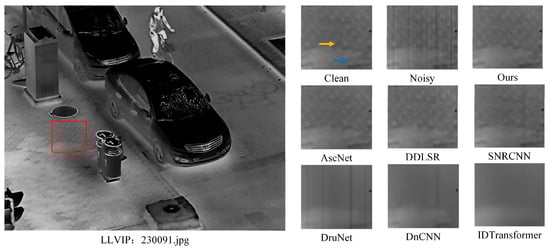
Figure 6.
Visual comparisons of different methods on the LLVIP dataset (1). For ease of observation, the texture of the details in the original image is enlarged to compare the denoising effects of different algorithms.
As shown in Figure 6, comparison regions are marked with red rectangles on the original images. To thoroughly validate method effectiveness, Level noise was introduced to this dataset. Selected regions are displayed in magnified comparative views.
As shown in Figure 7, comparison regions are annotated with red rectangles on source images. Level noise was introduced to this dataset to rigorously validate method efficacy. Magnified, detailed perspectives are provided for selected regions.
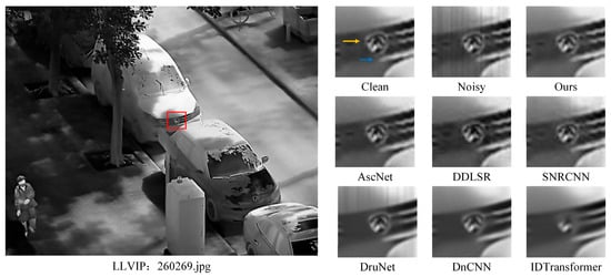
Figure 7.
Comparative visualization of different methods on the LLVIP dataset (2). For ease of observation, the texture of the details in the original image is enlarged to compare the denoising effects of different algorithms.
In the high-contrast images presented in Figure 7, both DnCNN and IDtransformer demonstrate superior denoising performance. This indicates their effectiveness when processing stripe noise with high edge separability, albeit with noticeable texture blurring. DruNet erroneously preserves certain stripe noises as structural edges, consequently introducing visual artifacts. At visual quality levels approaching clean reference images, both AscNet and our method achieve comparable performance.
As shown in Figure 8, comparison regions are annotated with red rectangles on source images. Leveled noise was introduced to this dataset to rigorously validate method efficacy.
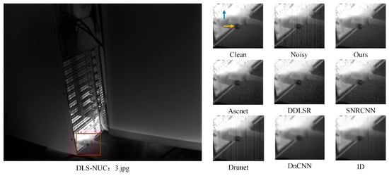
Figure 8.
Comparative visualization of different methods on the DLS-NUC dataset (1). For ease of observation, the texture of the details in the original image is enlarged to compare the denoising effects of different algorithms.
To validate the method’s effectiveness against high-intensity random noise, stronger Gaussian noise () was introduced to image “3.jpg” from the DLS-NUC dataset. The results are shown in Figure 8 and Figure 9. Comparative analysis focuses on the DVI interface area behind the host device. Experimental results demonstrate that the proposed method achieves optimal Gaussian noise suppression, with significantly less residual noise than comparative methods. While AscNet and DDLSR effectively remove stripe noise, they still retain substantial Gaussian noise components. Under strong Gaussian noise conditions, both IDtransformer and DruNet produce conspicuous artifacts, whereas DnCNN successfully eliminates all noise but leads to over-smoothed details. For image “23.jpg”, comparative analysis was conducted on the low-contrast railing area. It can be observed that all methods cause some degree of texture damage, whereas the proposed method achieves relatively optimal texture preservation capability among comparative algorithms.
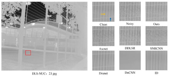
Figure 9.
Visual comparison of methods on DLS-NUC dataset (2). For ease of observation, the texture of the details in the original image is enlarged to compare the denoising effects of different algorithms.
As shown in Figure 9, comparative regions are indicated by red boxes on the original image. To fully demonstrate method effectiveness, graded noise was added to this dataset.
For image “004841.jpg” from the CVC09 dataset, stronger stripe noise () was introduced into the image, with results displayed in Figure 10 and Figure 11. The bridge-side guardrail area in this image was selected as the focus for comparative analysis. Among the evaluated methods, AscNet [20] and DDLSR [19] demonstrated superior denoising performance under strong stripe noise conditions. However, IDtransformer [23], DruNet [22], and DnCNN [21] were all observed to retain significant artifacts. Notably, the visual performance of the proposed method in terms of edge continuity and structural regularity approaches that of AscNet.
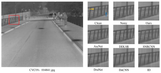
Figure 10.
Visual comparison of methods on CVC09 dataset (1). For ease of observation, the texture of the details in the original image is enlarged to compare the denoising effects of different algorithms.
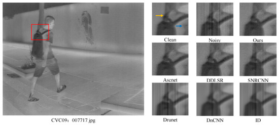
Figure 11.
Visual comparison of methods on CVC09 dataset (2). For ease of observation, the texture of the details in the original image is enlarged to compare the denoising effects of different algorithms.
In Figure 10, comparative regions are indicated by red boxes on the original image. To fully demonstrate method effectiveness, levels of noise were added to this dataset.
In Figure 11, comparative regions are indicated by red boxes on the original image. To fully demonstrate method effectiveness, levels of noise were added to this dataset.
For the image “007717.jpg”, the high-contrast backpack region was selected for further comparison. In terms of visual evaluation, both AscNet and the proposed method achieve favorable denoising effects, while DDLSR introduces excessive random noise leading to deteriorated image quality. SNRCNN fails to adequately identify the central region with severe strip noise, thus retaining noticeable artifacts.
To further demonstrate the robustness of the proposed method in real-world scenarios, in addition to artificially adding noise to infrared images, a set of infrared images captured by a self-developed camera was also added to the visualization experiment, as shown in Figure 12 and Figure 13. Due to the difficulty of obtaining clean images in real-world scenarios, GT is not added to the display image. In order to improve the visual effect, the denoising effect of the BM3D method is added to the comparison image.
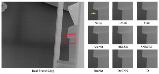
Figure 12.
The proposed method was compared visually on a self-developed camera dataset (1). For ease of observation, the texture of the details in the original image is enlarged to compare the denoising effects of different algorithms.
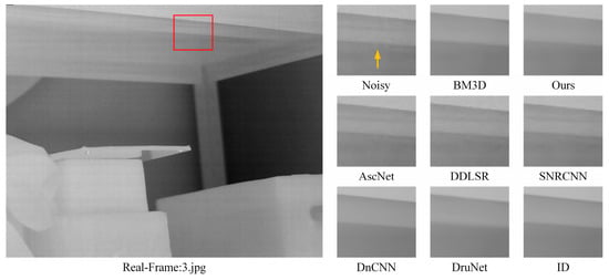
Figure 13.
The proposed method was compared visually on a self-developed camera dataset (2). For ease of observation, the texture of the details in the original image is enlarged to compare the denoising effects of different algorithms.
4.3. Quantitative Experiments
To validate the quantitative performance of the proposed method, this paper introduces multiple advanced methods for PSNR and SSIM comparison at noise level 6 (), 10 (), and 16 (), including BM3D [33], GTV [34], DruNet [22], DnCNN [21], IDTransformer [23], AscNet [20], DDLSR [19], and SNRCNN [16].
Overall, the self-attention mechanism based on IDTransformer exhibits excellent performance at low noise levels; however, with the enhancement of stripe noise, methods targeting point noise often perform poorly. Although AscNet, specifically designed for stripe noise, effectively removes stripe components, it retains too much random noise. Although deep learning methods such as IDTransformer, DruNet, AscNet, and DnCNN have achieved significant results in their respective professional tasks, their performance is still not optimal when dealing with mixed noise commonly present in real-world scenarios. This limitation may stem from differences in hyperparameter configuration between models, and in addition, changes in the operating environment may have an undeniable impact on performance. Specifically, under experimental conditions with a noise intensity of 15, the proposed method achieved maximum gains of 0.23 dB and 0.0108 dB on PSNR and SSIM, respectively, compared to the suboptimal model. It is worth noting that the proposed method exhibits significant advantages on the LLVIP dataset, which may be due to partial data distribution overlap between the dataset and the training set. Although the improvement on other datasets is relatively limited, it still outperforms all comparison methods, further validating the effectiveness and robustness of the proposed method. However, the advantages of LPIPS are not significant enough, which may be due to its tendency to measure high-frequency textures. Therefore, Ascnet and SNRCNN, which focus on stripe noise removal, have shown excellent results. The model design and loss function in this paper emphasize visual smoothing effects, suppressing noise while suppressing some high-frequency fine textures. In future work, we will improve this issue.
Table 1 presents quantitative comparisons with state-of-the-art methods on the test datasets. The best results are highlighted in bold, while the second-best results are underlined.

Table 1.
Quantitative comparisons with state-of-the-art methods on the test datasets. The better performance of different indicators are marked with “↑” and “↓”.
In Table 2, the NIQE and BRISQUE metrics for real images are provided to evaluate the effectiveness of the proposed method. This method achieved NIQE = 8.61 ± 1.16 and BRISQUE = 55.57 ± 5.04 without reference quality indicators, ranking among the top methods and significantly better than general denoising methods, such as GTV, BM3D, DnCNN, ID, and Drunet, and is close to the NIQE of SNRCNN (with a difference of 0.17). Meanwhile, the standard deviation of the proposed method is relatively small, indicating good stability across different scenarios.
Table 2.
Quantitative comparisons with state-of-the-art methods on the real-captured datasets, the better performance of different indicators are marked with “↓”.
4.4. Ablation Study
This section adopts the experimental configuration established in Section 4.1, with validation conducted under a noise level of 6.
4.4.1. Impact of Individual Loss Terms
Table 3 demonstrates the influence of different loss components on final model performance, where bold values denote best results. Experiments were conducted on three infrared datasets (LLVIP, CVC09, and DLS-NUC-100) with various loss function combinations. Results indicate that the joint application of three loss terms achieves optimal PSNR and SSIM across all datasets, yielding maximum improvements of up to 4.31 dB (PSNR) and 0.1435 (SSIM) compared to the second-best combination. This demonstrates significant complementary effects between the loss functions.
Table 3.
Ablation study of individual loss terms.
Employing loss alone provides a robust baseline model yet exhibits limited capability in enforcing structural consistency. When superimposing loss onto , SSIM on the CVC09 dataset significantly improves to 0.9215, while PSNR substantially decreases on both LLVIP and DLS-NUC-100 (31.72 dB and 33.72 dB, respectively), indicating that isotropic smoothing tends to cause over-suppression. Utilizing only the combination without a maintains high SSIM performance but leads to significant PSNR degradation, suggesting this scheme prioritizes structural preservation at the expense of smoothness. In contrast, the joint application of achieves optimal overall performance across all three datasets, validating effective complementarity and synergy among distinct loss components.
4.4.2. Impact of Edge Detection Weighting
Table 4 presents ablation studies on the effectiveness of edge detection weighting, where bold values denote best results. When this weighting is disabled, performance metrics decline across all three datasets, markedly evidenced by significant SSIM deterioration. This result indicates that the proposed adaptive weighting mechanism can effectively guide the CNN to alleviate excessive suppression of smoothing terms in edge regions, while more forcefully suppressing residual stripes and random noise in non-edge regions, without introducing additional parameters or increasing the complexity of the model architecture.
Table 4.
Ablation study on edge weights.
4.4.3. Impact of Different Network Architectures
Table 5 demonstrates the performance of the proposed optimized loss function across various network architectures (including UNet, DnCNN, FFDNet, DRUNet, and the ResNet used in this study) under controlled parameter scales (approximately 1.17 × 10⁴–1.31 × 10⁴), with non-denoised images as the baseline. The results indicate that all architectures significantly outperform the baseline after incorporating this loss function, with ResNet achieving the best performance (PSNR improvement of 4.68 dB; SSIM improvement of 0.1311), followed by DRUNet (PSNR improvement of 4.17 dB; SSIM improvement of 0.1260), while FFDNet shows relatively weaker performance (PSNR: 36.41; SSIM: 0.8874). The limitations of FFDNet may stem from its fundamental assumption, i.e., that noise follows a spatially independent zero-mean Gaussian distribution, whereas the fixed-pattern noise (FPN) in this task exhibits directional dependency, manifested as gain and offset components. In contrast, ResNet, with its layer-wise residual learning mechanism, can more effectively fit high-frequency stripe residuals and random noise while better preserving texture details.
Table 5.
Denoising performance across network architectures.
5. Conclusions
This study proposes a convolutional neural network denoising algorithm with a composite loss function to address mixed noise in real-world infrared images, rigorously validating its effectiveness. The method uses a residual network as the backbone, integrating adaptive weighting and edge preservation mechanisms to better model fixed-pattern noise (FPN).
Compared to classical methods like DnCNN, this approach eliminates reliance on clean images as supervisory signals. Instead, it achieves adaptive smoothing via the gradient variation characteristics of the image sequence itself, significantly reducing training data demands while improving adaptability to practical infrared imaging environments. Additionally, it offers a simplified solution for efficient hardware-side deployment of denoising networks.
Currently, while the method demonstrates strong denoising performance in multiple tests, its effectiveness may degrade in scenarios with highly similar training image backgrounds. This limitation stems from the spatial consistency of infrared FPN—even with superimposed Gaussian noise, insufficient local gradient variations hinder effective edge detection weight responses. Further research will investigate and refine this issue.
Author Contributions
Methodology, Y.T.; Software, J.L.; Validation, Y.T., C.M. and J.L.; Formal analysis, Y.T.; Investigation, C.M. and R.M.; Data curation, R.M.; Writing—original draft, C.M. and J.L.; Writing—review & editing, Y.T. and C.M.; Funding acquisition, R.M. All authors have read and agreed to the published version of the manuscript.
Funding
This research received no external funding.
Data Availability Statement
Data are contained within the article.
Conflicts of Interest
The authors declare no conflict of interest.
References
- Tang, W.; He, F.Z.; Liu, Y. TCCFusion: An infrared and visible image fusion method based on transformer and cross correlation. Pattern Recognit. 2023, 137, 109295. [Google Scholar] [CrossRef]
- Xia, C.Q.; Chen, S.H.; Huang, R.S.; Hu, J.; Chen, Z.M. Separable spatial-temporal patch-tensor pair completion for infrared small target detection. IEEE Trans. Geosci. Remote Sens. 2024, 62, 1–20. [Google Scholar] [CrossRef]
- Tang, W.; He, F.Z.; Liu, Y.; Duan, Y.S.; Si, T.Z. DATFuse: Infrared and visible image fusion via dual attention transformer. IEEE Trans. Circuits Syst. Video Technol. 2023, 33, 3159–3172. [Google Scholar] [CrossRef]
- Luo, Y.; Li, X.R.; Chen, S.H.; Xia, C.Q. LEC-MTNN: A novelmulti-frame infrared small target detection method based on spatial-temporal patch-tensor. In Earth and Space: From Infrared to Terahertz, ESIT 2022; SPIE: Bellingham, WA, USA, 2023; Volume 12505, pp. 144–154. [Google Scholar]
- Zhang, C.; Zhao, W.Y. Scene-based nonuniformity correction using local constant statistics. J. Opt. Soc. Am. A 2008, 25, 1444–1453. [Google Scholar] [CrossRef]
- Li, Z.; Luo, S.J.; Chen, M.; Wu, H.; Wang, T.; Cheng, L. Infrared thermal imaging denoising method based on second-order channel attention mechanism. Infrared Phys. Technol. 2021, 116, 103789. [Google Scholar] [CrossRef]
- Yang, P.F.; Wu, H.; Cheng, L.L.; Luo, S.J. Infrared image denoising via adversarial learning with multi-level feature attention network. Infrared Phys. Technol. 2023, 128, 104527. [Google Scholar] [CrossRef]
- Feng, T.; Jin, W.Q.; Si, J.J. Spatial-noise subdivision evaluation model of uncooled infrared detector. Infrared Phys. Technol. 2021, 119, 103954. [Google Scholar] [CrossRef]
- Wang, E.; Liu, Z.; Wang, B.; Cao, Z.Y.; Zhang, S.W. Infrared image stripe noise removal using wavelet analysis and parameter estimation. J. Mod. Opt. 2023, 70, 170–180. [Google Scholar] [CrossRef]
- He, Y.F.; Zhang, C.M.; Zhang, B.Y.; Chen, Z.Y. FsPnP: Plug-and-Play frequency-spatial-domain hybrid denoiser for thermal infrared image. IEEE Trans. Geosci. Remote Sens. 2024, 62, 5000416. [Google Scholar] [CrossRef]
- Li, J.; Liu, K.Y.; Hu, Y.T.; Zhang, H.C.; Heidari, A.A.; Chen, H.; Zhang, W.J.; Algarni, A.D.; Elmanna, H. Eres-UNet plus Liver CT image segmentation based on high efficiency channel attention and Res-UNet plus. Comput. Biol. Med. 2023, 158, 106501. [Google Scholar] [CrossRef]
- Li, J.; Wang, J.W.; Lin, F.W.; Wu, W.Q.; Chen, Z.M.; Heidari, A.A.A.; Chen, H.L. DSEUNet: A lightweight UNet for dynamic space grouping enhancement for skin lesion segmentation. Expert Syst. Appl. 2024, 255, 124544. [Google Scholar] [CrossRef]
- Li, J.; Kang, J.R.; Qi, J.; Fu, H.K.; Liu, B.Q.; Lin, X.L.; Zhao, J.W.; Guan, H.X.; Chang, J. Soybean yield estimation using improved deep learning models with integrated multisource and multitemporal remote sensing data. IEEE J. Sel. Top. Appl. Earth Obs. Remote Sens. 2025, 18, 18450–18477. [Google Scholar] [CrossRef]
- Yang, F.; Chen, X.; Chai, L. Hyperspectral image destriping and denoising using stripe and spectral low-rank matrix recovery and global spatial–spectral total variation. Remote Sens. 2021, 13, 827. [Google Scholar] [CrossRef]
- Kang, M.; Jung, M. Nonconvex fractional-order total variation based image denoising model under mixed stripe and Gaussian noise. AIMS Math. 2024, 9, 21094–21124. [Google Scholar] [CrossRef]
- Ding, D.; Li, Y.; Zhao, P.; Li, K.T.; Jiang, S.; Liu, Y.X. Single infrared image stripe removal via residual attention network. Sensors 2022, 22, 8734. [Google Scholar] [CrossRef]
- Wu, X.B.; Zheng, L.L.; Liu, C.Y.; Gao, T.; Zhang, Z.; Yang, B. Single-image simultaneous destriping and denoising: Double low-rank property. Remote Sens. 2023, 15, 5710. [Google Scholar] [CrossRef]
- Chang, Y.; Yan, L.X.; Liu, L.; Fang, H.; Zhong, S. Infrared aerothermal nonuniform correction via deep multiscale residual network. IEEE Geosci. Remote Sens. Lett. 2019, 16, 1120–1124. [Google Scholar] [CrossRef]
- Kuang, X.D.; Sui, X.B.; Liu, Y.; Liu, C.W.; Chen, Q.; Gu, G.H. Robust destriping method based on data-driven learning. Infrared Phys. Technol. 2018, 94, 142–150. [Google Scholar] [CrossRef]
- Yuan, S.; Qin, H.L.; Yan, X.; Yang, S.Q.; Yang, S.W.; Akhtar, N.; Zhou, H.X. AscNet: Asymmetric sampling correction network for infrared image destriping. IEEE Trans. Geosci. Remote Sens. 2025, 63, 5001815. [Google Scholar] [CrossRef]
- Zhang, K.; Zuo, W.M.; Chen, Y.J.; Meng, D.Y.; Zhang, L. Beyond a Gaussian denoiser: Residual learning of deep CNN for image denoising. IEEE Trans. Image Process. 2017, 26, 3142–3155. [Google Scholar] [CrossRef] [PubMed]
- Zhang, K.; Li, Y.W.; Zuo, W.M.; Zhang, L.; Van Gool, L.; Timofte, R. Plug-and-play image restoration with deep denoiser prior. IEEE Trans. Pattern Anal. Mach. Intell. 2022, 44, 6360–6376. [Google Scholar] [CrossRef] [PubMed]
- Shen, Z.W.; Qin, F.W.; Ge, R.Q.; Wang, C.M.; Zhang, K.; Huang, J. IDTransformer: Infrared image denoising method based on convolutional transposed self-attention. Alex. Eng. J. 2025, 110, 310–321. [Google Scholar] [CrossRef]
- Chen, Y.; Huang, T.Z.; Zhao, X.L.; Deng, L.J.; Huang, J. Stripe noise removal of remote sensing images by total variation regularization and group sparsity constraint. Remote Sens. 2017, 9, 559. [Google Scholar] [CrossRef]
- Yang, J.H.; Zhao, X.L.; Ma, T.H.; Chen, Y.; Huang, T.Z.; Ding, M. Remote sensing images destriping using unidirectional hybrid total variation and nonconvex low-rank regularization. J. Comput. Appl. Math. 2020, 363, 124–144. [Google Scholar] [CrossRef]
- Chen, H.; Zhao, L.; Liu, T.T.; Sun, X.C.; Liu, H. Flexible infrared image destriping algorithm with L1-based sparse regularization for wide-field astronomical images. Infrared Phys. Technol. 2022, 125, 104297. [Google Scholar] [CrossRef]
- Hu, X.R.; Luo, S.J.; He, C.H.; Wu, W.H.; Wu, H. Infrared thermal image denoising with symmetric multi-scale sampling network. Infrared Phys. Technol. 2023, 134, 104909. [Google Scholar] [CrossRef]
- Lee, H.; Kang, M.G. Infrared image deconvolution considering fixed pattern noise. Sensors 2023, 23, 3033. [Google Scholar] [CrossRef]
- Pan, E.; Ma, Y.; Mei, X.G.; Huang, J.; Chen, Q.H.; Ma, J.Y. Hyperspectral image destriping and denoising from a task decomposition view. Pattern Recognit. 2023, 144, 109832. [Google Scholar] [CrossRef]
- Wang, M.H.; Yuan, P.; Qiu, S.; Jin, W.Q.; Li, L.; Wang, X. Dual-encoder UNet-based narrowband uncooled infrared imaging denoising network. Sensors 2025, 25, 1476. [Google Scholar] [CrossRef]
- Huang, Z.H.; Zhu, Z.F.; Wang, Z.C.; Li, X.; Xu, B.Y.; Zhang, Y.Z.; Fang, H. D3cNNs: Dual denoiser driven convolutional neural networks for mixed noise removal in remotely sensed images. Remote Sens. 2023, 15, 443. [Google Scholar] [CrossRef]
- Liu, K.; Chen, H.L.; Bao, W.Z.; Wang, J.L. Thermal imaging spatial noise removal via deep image prior and step-variable total variation regularization. Infrared Phys. Technol. 2023, 134, 104888. [Google Scholar] [CrossRef]
- Dabov, K.; Foi, A.; Katkovnik, V.; Egiazarian, K. Image denoising by sparse 3-D transform-domain collaborative filtering. IEEE Trans. Image Process. 2007, 16, 2080–2095. [Google Scholar] [CrossRef] [PubMed]
- Yi, X.; Min, C.B.; Shao, M.C.; Zheng, H.J.; Lv, Q.F. Low-Light Image Enhancement via Regularized Gaussian Fields Model. Neural Process. Lett. 2023, 55, 12017–12037. [Google Scholar] [CrossRef]


Disclaimer/Publisher’s Note: The statements, opinions and data contained in all publications are solely those of the individual author(s) and contributor(s) and not of MDPI and/or the editor(s). MDPI and/or the editor(s) disclaim responsibility for any injury to people or property resulting from any ideas, methods, instructions or products referred to in the content. |
© 2025 by the authors. Licensee MDPI, Basel, Switzerland. This article is an open access article distributed under the terms and conditions of the Creative Commons Attribution (CC BY) license (https://creativecommons.org/licenses/by/4.0/).