Abstract
The increasing scale and complexity of graph-structured data necessitate efficient parallel training strategies for graph neural networks (GNNs). The effectiveness of these strategies hinges on the quality of graph feature representation. To this end, we propose a Frequency-Adaptive Dual-Pooling Graph Transformer (FADP-GT) model to enhance feature learning for computational graphs. We propose a Frequency-Adaptive Dual-Pooling Graph Transformer (FADP-GT) model, which incorporates two modules: a Frequency-Adaptive Graph Attention (FAGA) module and a Dual-Pooling Feature Refinement (DPFR) module. The FAGA module adaptively filters frequency components in the spectral domain to dynamically adjust the contribution of high- and low-frequency information in attention computation, thereby enhancing the model’s ability to capture structural information and mitigating the over-smoothing problem in multi-layer network propagation. On the other hand, the DPFR module refines graph features through dual-pooling operations—Global Average Pooling (GAP) and Global Max Pooling (GMP)—along the node dimension, which captures both global feature distributions and salient local patterns to enrich multi-scale representations. By improving graph feature representation, our FADP-GT model indirectly supports the development of efficient device placement strategies, as enhanced feature extraction enables the more accurate modeling of node dependencies in computational graphs. The experimental results demonstrate that FADP-GT outperforms existing methods, reducing the average computation time for device placement by 96.52% and the execution time by 9.06% to 26.48%.
1. Introduction
In recent years, large-scale neural network models have demonstrated a remarkable performance across various complex tasks, such as high-accuracy image classification [1,2,3], intelligent speech recognition [4,5,6], and efficient machine translation [7,8,9]. Their strong performance stems from these models’ ability to extract and learn complex feature relationships from large-scale datasets. However, as the computational demands during training and inference grow rapidly, the scale of neural network models continues to expand significantly.
For instance, OpenAI’s GPT-3 model [10], with 175 billion parameters, presents significant training challenges. Training such an ultra-large model is not only time-consuming but also demands computational resources that far exceed the capabilities of traditional hardware. As a result, conventional single-machine training is clearly inadequate for models of this scale.
In light of this, developing efficient and suitable distributed training approaches has become imperative. Distributed training allocates training tasks across multiple computing devices for parallel execution, thereby significantly improving training efficiency. Current research focuses on designing and selecting effective distributed parallelization strategies to accelerate the training process of neural network models. Through rational parallelization strategies, we can fully utilize the computational power of multiple devices, optimizing resource allocation and reducing training time.
Currently, distributed parallelization strategies are primarily categorized into two types: those designed manually based on expert experience and those automatically generated via algorithms. Expert-driven manual design relies on the deep knowledge of domain professionals to tailor parallelization schemes for specific models and tasks. Although expert-driven design can yield satisfactory results in specific scenarios, it becomes increasingly impractical for optimizing modern, complex neural networks.
In contrast, automated search techniques offer a more scalable and efficient alternative. These methods leverage algorithms to explore the vast space of possible parallelization strategies, identifying near-optimal configurations with minimal human intervention. Automatic search technology in parallel paradigms mainly includes data parallelism [11,12] and model parallelism [13,14]. Data parallelism accelerates by splitting data, but it is only applicable when the model scale is smaller than the memory of a single device; when the model scale exceeds the memory of a single device (such as GPT-3), model parallelism is required to split the model into sub-models and allocate them to different devices—the “sub-model–device” mapping process comprises device placement, and the quality of the placement strategy directly influences the communication and computational efficiency of model parallelism, so it is necessary to design efficient device placement algorithms.
Early research on model parallelism, such as the 2017 study by Mirhoseini et al. that applied reinforcement learning to device placement in data flow graphs, achieved significant reductions in runtime [15]. Subsequent studies, including hierarchical device placement (HDP) [16] and Spotlight [17], further enhanced scalability while minimizing training overhead. However, these methods still encounter difficulties in capturing long-range dependencies when processing large graph-structured data.
In recent years, approaches combining graph neural networks (GNNs) [18] with reinforcement learning (RL) [19,20,21] have opened new avenues for addressing model parallelism challenges. For example, Addanki et al.’s method, Placeto [22], pioneered the use of graph embedding networks for device placement. Methods such as GDP [23], GraphSAGE [24], and P-GNN [24] have further enhanced the performance of GNNs by incorporating neighborhood aggregation, random sampling, and positional embedding techniques.
However, traditional GNNs still suffer from an imprecise perception of structural information, over-smoothing in multi-layer propagation, and limited feature representation when processing complex graph-structured data, resulting in suboptimal device placement strategies. Insufficient structural perception may lead the model to misjudge data dependencies between computational nodes, assign highly interdependent nodes to different GPUs, and thereby increase cross-device communication delays. Over-smoothing will homogenize the features of computing nodes, making it impossible to distinguish between nodes with high computing power requirements and nodes with low computing power requirements, resulting in an unbalanced device load. To address these limitations, we propose a Frequency-Adaptive Dual-Pooling Graph Transformer (FADP-GT) model that integrates frequency graph theory with multi-scale feature fusion. By incorporating a Frequency-Adaptive Graph Attention (FAGA) module and a Dual-Pooling Feature Refinement (DPFR) module, our model provides a novel solution to device placement problems. The experimental results demonstrate that the FADP-GT model significantly outperforms existing methods in device placement for computational graphs.
The main contributions of this study are as follows:
- We propose the Frequency-Adaptive Graph Attention (FAGA) module, which incorporates frequency graph theory into an attention mechanism. By decomposing the graph adjacency matrix and adaptively filtering high- and low-frequency components, FAGA enhances the model’s capacity to capture both local and global structural dependencies, effectively mitigating over-smoothing.
- We design the Dual-Pooling Feature Refinement (DPFR) module, which leverages both Global Average Pooling and Global Max Pooling operations along the node dimension. This design enriches multi-scale feature representations by simultaneously capturing overall feature distributions and salient patterns, leading to more refined graph embeddings.
- Through extensive experiments on synthetic benchmarks (ptb, cifar10, nmt), we demonstrate that FADP-GT significantly outperforms existing state-of-the-art methods. Our model achieves a reduction in execution time of 9.06% to 26.48% and a dramatic decrease of 96.52% in the computation time required to search for the optimal placement strategy.
2. Methods
In response to the growing demand for the efficient processing of graph-structured data in the field of graph neural networks, this paper proposes a Frequency-Adaptive Dual-Pooling Graph Transformer (FADP-GT) model that integrates modules. The complete process is shown in Figure 1. Through the co-design of the Frequency Adaptive Graph Attention (FAGA) module and the Dual Pooling Feature Refinement (DPFR) module, the FADP-GT model significantly improves the representation capability and task performance of graph data.
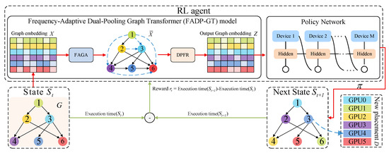
Figure 1.
The FADP-GT model performs the overall process of device placement strategy searching and optimization based on a reinforcement learning mechanism.
Complex neural networks are modeled as a directed acyclic graph G with N nodes, where each node represents a specific computational operation, and a set D containing M devices is defined to denote available computing resources. From G, a node feature matrix (where N denotes the number of computational nodes and d is the initial dimension of node features) and an adjacency matrix are derived and input into the FAGA module to obtain a projected feature matrix (where represents the feature dimension after projection), with the data flow expressed as . Subsequently, is input into the DPFR module to generate an enhanced graph embedding ; this process is denoted as .
Next, the enhanced graph embedding is fed into the Policy Network to generate a device placement policy , and thereby forms the state , with the data flow expressed as . The policy is executed on the target GPU configuration, and the execution times for states and are measured to assess performance. The resulting reward signal is then computed and fed back via backpropagation to update the Policy Network, FAGA, and DPFR modules, thereby optimizing the device placement strategies. This iterative optimization continues until the execution time stabilizes, ultimately achieving the goal of efficient device placement. The entire process can be summarized as .
2.1. Problem Definition
Traditional graph neural networks (GNNs) face three critical challenges when handling graph-structured data in device placement tasks:
- Insufficient structural perception: Standard graph neural networks often rely on localized neighborhood aggregation, which limits their ability to capture long-range dependencies and global topological patterns in computational graphs. This leads to the suboptimal modeling of node correlations critical for device placement, such as failing to identify communities of nodes that should be co-located.
- Over-smoothing in multi-layer propagation: As the number of network layers increases, node features tend to become homogeneous, reducing their discriminability and further degrading the accuracy of device placement strategies.
- Limited feature representation: Conventional GNNs fail to capture the multi-scale information (global distribution vs. local salient patterns) of graph features, resulting in suboptimal placement decisions.
To address these issues, our FADP-GT model innovatively integrates spectral graph theory and multi-scale feature fusion through two core modules: the Frequency-Adaptive Graph Attention (FAGA) module (targeting challenges 1 and 2) and the Dual-Pooling Feature Refinement (DPFR) module (targeting challenge 3).
2.2. Frequency-Adaptive Graph Attention (FAGA) Module
The FAGA module dynamically adjusts the contributions of high- and low-frequency components in the attention mechanism by performing a frequency decomposition of the adjacency matrix. This enhances the model’s ability to capture structural information and mitigates over-smoothing. As illustrated in Figure 2, the FAGA module takes node features and the adjacency matrix as inputs, performs frequency decomposition, and adaptively fuses frequency components to modulate the attention mechanism.
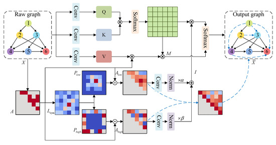
Figure 2.
Schematic diagram of the Frequency-Adaptive Graph Attention (FAGA) module. The module takes node features and the adjacency matrix as inputs, performs frequency decomposition to obtain high- and low-frequency components, adaptively weights them, and uses the fused frequency information to modulate the standard attention computation.
2.2.1. Feature Mapping and Structural Modulation
Given the input node feature matrix , where N denotes the number of nodes and d is the dimension of node features, along with the adjacency matrix describing the connectivity between nodes, we first project into query (), key (), and value () matrices through linear transformations:
where , , and are learnable weight matrices, and represents the dimension of the mapped features.
To incorporate structural information into the attention computation, we adjust the standard mechanism by constructing a structural modulation matrix as follows:
where the adjacency matrix constrains the interactions between value vectors , ensuring that the attention mechanism focuses more on node pairs connected by edges.
2.2.2. Frequency Decomposition and Adaptive Filtering
Though FADP-GT’s frequency-adaptive filtering and classical GCN both fall into graph signal processing based on the graph Laplacian, their core difference is clear. Classical GCN focuses on “local neighborhood aggregation + Laplacian smoothing.” In its default implementation, it does not explicitly split low- and high-frequency signals, but rather indirectly processes the graph’s overall frequency range through local aggregation. Essentially, it filters noise through the Laplacian’s smoothing property, yet lacks explicit frequency splitting, independent modeling of low/high-frequency components, and frequency-specific weight adjustment. In contrast, FADP-GT’s mechanism achieves precise low/high-frequency regulation via explicit decomposition, dynamic weight learning, and feature calibration.
We perform an eigen-decomposition of the normalized graph Laplacian to project the graph structure into the spectral domain, enabling the explicit modeling and separate processing of low- and high-frequency information. Low-frequency components emphasize global smoothness and community structure, guiding tightly connected node groups to the same device to minimize communication. High-frequency components highlight local variations and critical dependencies, ensuring that bottleneck operations are correctly identified and placed. This decomposition lets the model adaptively balance these complementary structural cues.
Frequency-adaptive filtering is implemented by decomposing the adjacency matrix into high- and low-frequency components, as detailed below:
First, the graph Laplacian matrix is computed as , then symmetrically normalized:
where is the degree matrix. Symmetric normalization ensures that is a real symmetric matrix, facilitating subsequent frequency analysis.
The normalized Laplacian matrix is then eigen-decomposed to obtain eigenvalues and corresponding eigenvectors . A threshold is set to partition the eigenspace into a low-frequency subspace (corresponding to smaller eigenvalues, ) and a high-frequency subspace (corresponding to larger eigenvalues, ). Accordingly, the low- and high-frequency projection matrices are constructed:
Based on the projection matrices, the low- and high-frequency adjacency components and are derived:
To adaptively regulate the contribution of each frequency component in the attention computation, two learnable parameters are introduced: (weight of low-frequency component) and (weight of high-frequency component). The weights satisfy (normalized via Softmax to ensure balanced contributions).
First, Layer Normalization is applied to the low-frequency adjacency component and high-frequency adjacency component to stabilize training. Then, a 1 × 1 convolution is employed to align the channel dimension of the normalized components with the attention matrix’s dimension, enhancing their expressive power:
where is the frequency component after fusion. By training learnable parameters and , they are adaptively adjusted through backpropagation training, enabling the model to dynamically balance the contribution of each frequency component based on the input graph.
The weighted high- and low-frequency components are used to adjust the query–key affinity matrix, yielding the output of the FAGA module:
2.3. Dual-Pooling Feature Refinement (DPFR) Module
The DPFR module employs Global Average Pooling (GAP) and Global Max Pooling (GMP) along the node dimension to generate two distinct global context vectors. These operations refine the node features by capturing complementary aspects of the feature distribution. The implementation details of the DPFR module are shown in Figure 3.
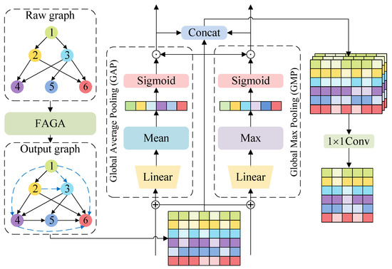
Figure 3.
Architecture of the Dual-Pooling Feature Refinement (DPFR) module. The module takes the output of the FAGA module and applies parallel Global Average Pooling (GAP) and Global Max Pooling (GMP) branches. The resulting context vectors are used to calibrate the features, which are then concatenated and projected to produce the final refined output.
Specifically, Global Average Pooling focuses on capturing the overall distribution of node features, while Global Max Pooling emphasizes extracting salient patterns in node features. Based on these two types of contextual information, recalibrated feature maps and are generated, refining node features from different angles. The original features are then concatenated with the refined features to preserve complete feature information, followed by a 1 × 1 convolution for cross-channel linear projection, fusing multi-channel information into a unified feature space:
where and are GAP and GMP feature maps at time step i, represents the integration of multi-channel information into a unified feature space, and signifies the enhanced node features.
2.3.1. Global Average Pooling (GAP) Branch
The GAP branch captures the overall distribution of node features through average pooling. This process results in a vector that is expanded through a linear layer to generate a weight vector, which adaptively scales the original features to emphasize important characteristics. The recalibrated feature map is obtained as follows:
where denotes the global average context vector; is used as the adaptive weight vector for the GAP branch.
2.3.2. Global Max Pooling (GMP) Branch
The GMP branch extracts salient patterns within the features through max pooling. Similarly, a weight vector is generated via a linear layer followed by a Sigmoid activation, producing the recalibrated feature map to enhance the representation of critical features:
where denotes the global max context vector; is used as the adaptive weight vector for the GMP branch.
2.4. Reinforcement Learning Integration for Device Placement
The FADP-GT model takes the enhanced graph embedding as the core input to a reinforcement learning (RL) framework, realizing end-to-end generation and the optimization of device placement strategies in line with the Markov Decision Process (MDP) paradigm. The overall workflow aligns with the model architecture illustrated in Figure 1 for Policy Generation.
2.4.1. From to Placement Strategy
The enhanced graph embedding is fed into the Policy Network, which maps to a logit matrix (unnormalized node–GPU assignment probabilities: rows for nodes, columns for GPUs). A sampling function converts logits to the placement strategy (each denotes the target GPU of node i): during training, an epsilon-greedy strategy (with a fixed seed for reproducibility) balances exploration (polynomial sampling) and exploitation; during evaluation, the highest-probability GPU is selected via argmax for a stable performance.
2.4.2. State Transition and Policy Execution
This part describes how the MDP state transitions and the placement strategy is executed. Each MDP state includes , binary ’visited’ node flags, and one-hot vectors for GPU counts (3/5/8 GPUs). Once is generated, all nodes are marked as ’visited’ to transition to . The strategy is then executed on GPUs, with an event-based simulator measuring .
2.4.3. Reward Calculation and Parameter Update
The intermediate reward is calculated to evaluate the quality of the placement strategy, considering both the reduction in execution time and penalties for memory overflow:
where c is the memory overflow penalty factor, is the peak memory of the state, and O is the maximum GPU memory.
To establish the link between and the reward optimization objective, we adopt the policy gradient theorem and define the RL objective as maximizing the expected cumulative reward over episodes:
where denotes the combined parameters of the Policy Network, FAGA, and DPFR modules, (discount factor for future rewards), and T is the number of steps per episode. The policy gradient is computed as
where is the log-probability of action (node–GPU assignment) given state (dependent on ), establishing a direct mathematical connection between and the reward gradient.
The reward and policy gradient are backpropagated without truncation to update the Policy Network, FAGA, and DPFR modules simultaneously—this ensures gradients from RL effectively propagate to early parameters in FAGA/DPFR. This iterative loop (generation → execution → reward → update) continues until the stabilizes, achieving efficient device placement.
3. Experiment and Analysis
In this section, we provide a comprehensive overview of the experimental setup, present detailed results, and offer an in-depth analysis to validate the effectiveness and efficiency of the proposed FADP-GT model. The insights gained from evaluations across multiple datasets and device configurations are thoroughly discussed.
3.1. Experimental Setup
To comprehensively evaluate the efficacy of the proposed model, we structure the experimental setup across three interconnected dimensions: the dataset configuration, evaluation metrics, and the hardware/software environment. The details of each dimension are elaborated as follows.
3.1.1. Dataset Configuration
We utilize computational graphs derived from three representative benchmarks to cover diverse model architectures:
ptb: Models recurrent neural networks (RNNs) [25,26] for language modeling tasks.
cifar10: Models convolutional neural networks (CNNs) [27] for image classification tasks.
nmt: Models neural machine translation (NMT) [28,29] systems for sequence-to-sequence tasks.
For each benchmark, we generate 17 input computational graphs with fixed structural parameters. The key structural metrics of the graphs are shown in Table 1.

Table 1.
Structural metrics of computational graphs for each benchmark.
To ensure result stability and reproducibility, all graph generation processes use a fixed random seed, which standardizes node connection relationships, feature initialization, and layer dependency mapping across experimental runs. Each computational graph is further used in 20 training epochs, where consistent seed sequences are applied for batch sampling and parameter initialization, to mitigate random variance.
3.1.2. Evaluation Metrics
We adopt two key metrics to assess performance from complementary perspectives.
Execution Time: Precisely indicates the total duration needed to train a neural network after applying a device placement policy based on a specific graph embedding technique. This duration covers all key stages of the training process guided by the policy: data loading, model forward propagation, model backward propagation, cross-device communication, and parameter updating (i.e., the full workflow of neural network training post policy application). Measurement details: captured via NVIDIA Nsight Systems (v2023.3), with the results averaged over 10 independent runs to mitigate random variance (unit: seconds).
Computation Time: Measures the total duration required to find the optimal device placement policy. This includes two core stages of policy search: reinforcement learning (RL) agent training (i.e., updating the Policy Network to learn effective placement patterns) and strategy validation (i.e., evaluating candidate policies on validation graphs to screen out the optimal one). Measurement details: excludes data preprocessing time (irrelevant to policy search), with the results averaged over five independent runs to ensure reliability (unit: seconds).
3.1.3. Hardware and Software Environment
The experiments are conducted on a dedicated server with the following specifications:
Software Stack: Python: 3.6.13; TensorFlow: 1.12.0; CUDA: V9.0.176; cuDNN: v7.3.1.
Hardware Components: CPU: Intel(R) Xeon(R) CPU E5-2650 v4 @ 2.20GHz; GPU: Tesla P100; Memory: 128GB; Operating System: Ubuntu 18.04.4 LTS (64-bit).
To simulate scalable resource environments in distributed training, all experiments are executed under three GPU configurations: three, five, and eight GPUs.
3.2. Comparison of FADP-GT with State-of-the-Art Methods on Device Placement
We compared the proposed FADP-GT model against several state-of-the-art methods, including Placeto [22], GraphSAGE [24], P-GNN [24], GNN [18], GCN [30], GAT [31], Graphormer [32], and Mamba [33]. The results, summarized in Table 2, demonstrate consistent and significant improvements in execution time across all datasets and GPU configurations.
Table 2.
The execution time and improvement percentage of different methods on various datasets with different numbers of GPUs.
With the ptb dataset, FADP-GT achieved the shortest execution times across all GPU configurations (4.9757 s with three GPUs, 4.8378 s with five GPUs, and 4.6792 s with eight GPUs). Compared with Placeto, this represents a reduction in execution time of 12.08%, 13.22%, and 15.13%, respectively. Similarly, with cifar10, FADP-GT recorded execution times of 1.6885 s with three GPUs, 1.5916 s using five GPUs, and 1.5335 s with eight GPUs, achieving improvements of 19.83%, 26.48%, and 21.80% over the Placeto method. For the nmt dataset, FADP-GT achieved 2.0201 s with three GPUs, 1.9070 s with five GPUs, and 1.8805 s with eight GPUs, corresponding to improvements of 12.69%, 9.06%, and 11.44% over the same baseline.
To further demonstrate the effectiveness of the Frequency-Adaptive Dual-Pooling Graph Transformer (FADP-GT) model, we plotted a trend figure of execution time versus training episodes for different models under various datasets (ptb, cifar10, nmt) and different GPU configurations (three GPUs, five GPUs, eight GPUs), as shown in Figure 4. One episode is a full reinforcement learning (RL) cycle: (1) generate placement policy via the Policy Network using FAGA/DPFR-processed embedding ; (2) execute with synchronous SGD (fixed learning rate 0.001), obtain , measure execution time; (3) calculate reward (time reduction minus memory penalty) and apply reward smoothing via threshold clipping; (4) update all modules post episode.
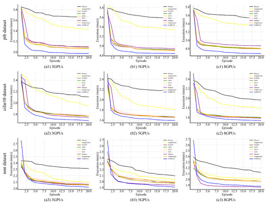
Figure 4.
The execution time of various comparison models under distinct episodes.
In Figure 4, the execution time of all compared models shows a consistent trend of gradually decreasing with the increase in training episodes and eventually stabilizing, which aligns with the logic of models optimizing device placement strategies through iteration under the reinforcement learning mechanism. Moreover, across all “dataset–GPU configuration” combination scenarios, the execution time of FADP-GT consistently exhibits significant advantages: its initial execution time is lower than that of other compared models, its speed of converging to a stable state is faster than that of other models, and its execution time after stabilization is also lower than that of all baseline models. Meanwhile, from the dataset perspective, the relative improvement in FADP-GT’s execution time in scenarios involving the cifar10 dataset is greater than that in scenarios involving the ptb and nmt datasets; from the GPU configuration perspective, as the number of GPUs increases, the reduction in FADP-GT’s execution time shows a gradually expanding trend, which reflects the model’s strong adaptability to multi-device parallel environments.
In terms of computation time, as presented in Table 3, FADP-GT also exhibited substantial advantages. Compared with Placeto, it reduced the average computation time by 97.69% with three GPUs, 97.77% using five GPUs, and 97.58% with eight GPUs on ptb; by 97.21%, 97.09%, and 97.07% on cifar10 across the three GPU configurations; and by 94.92%, 94.78%, and 94.61% on nmt. Although simpler models such as GNN and GCN showed marginally lower computation times due to their less complex architectures, FADP-GT maintained a favorable balance between performance and efficiency, underscoring its practical utility.
Table 3.
The computation time and improvement percentage of different methods on various datasets with different numbers of GPUs.
The superior performance of FADP-GT in execution time stems from two key design innovations. First, the FAGA module dynamically adjusts the contributions of high-frequency components that capture local dependencies and sharp transitions and low-frequency components that reflect global community structure through frequency decomposition of the adjacency matrix. This enables the model to better capture both long-range dependencies—for example identifying node communities for co-location—and fine-grained local patterns such as critical bottleneck operations, significantly improving the accuracy of feature extraction for device placement. Second, the DPFR module refines features by using Global Average Pooling (GAP) and Global Max Pooling (GMP). The GAP branch focuses on capturing the overall distribution of node features, while the GMP branch extracts salient patterns from node features. This Dual-Pooling Feature Refinement mechanism not only effectively mitigates over-smoothing during node aggregation but also enriches graph embeddings by dynamically balancing global and local feature contributions, resulting in more precise and efficient device placement strategies.
In terms of computation time, FADP-GT also demonstrates significant advantages over models such as Placeto, GraphSAGE, and P-GNN. Although simpler models like GNN, GCN, and GAT have slightly lower computation times due to their less complex architectures, FADP-GT’s computation time remains competitive in most scenarios. This efficiency stems from FADP-GT’s holistic feature extraction from the entire graph, as opposed to processing nodes or edges individually, ensuring a high performance while maintaining computational efficiency.
3.3. Ablation Study on the Frequency-Adaptive Graph Attention (FAGA) Module for Device Placement
To systematically evaluate the impact of various branch combinations within the FAGA module on model performance, we employed the Transformer [29] as the baseline model. Ablation studies were conducted to analyze how different configurations, including the adjacency matrix, high-frequency branch, and low-frequency branch, affect model execution time, with the detailed results presented in Table 4.
Table 4.
Ablation experiment results for adjacency matrix and spectrum branch in FAGA module under different datasets and GPU configurations.
We first evaluated the contribution of the FAGA module using the Transformer as the baseline (Index 1). Introducing the adjacency matrix alone (Index 2) improved the execution time by an average of 0.58% on ptb, 0.51% on cifar10, and 0.92% on nmt compared with Index 1, confirming that structural information enhances node correlation modeling.
When the high-frequency branch was introduced alone (Index 3), the execution time improved by 0.64% to 1.11% on ptb, 0.79% to 1.29% on cifar10, and 1.20% to 2.41% on nmt compared with Index 2. This indicates that the high-frequency branch effectively exploits high-frequency components in the graph structure, which accentuate local variations and critical dependencies, ensuring that unique and bottleneck operations are correctly identified and placed to avoid performance degradation.
Introducing only the low-frequency branch (Index 4) yielded less notable improvements in execution time on ptb and nmt compared with Index 3. However, for cifar10, the performance gains surpassed those of the high-frequency branch alone, with improvements of approximately 1.08%, 1.15%, and 0.95% under the three GPU, five GPU, and eight GPU configurations, respectively. This suggests that the structural characteristics of the cifar10 computational graphs are more effectively captured by low-frequency components, which emphasize global smoothness and community structure, guiding the placement of tightly connected node groups onto the same device to minimize communication.
Combining both high- and low-frequency branches (Index 5) led to better execution times than using either branch alone. For example, on the ptb dataset with a three GPU configuration, the execution time improved from 5.0257 s (Index 3) to approximately 5.0118 s (Index 5). Similar improvements were observed for the cifar10 and nmt datasets. This indicates that the combination of high- and low-frequency components captures a broader range of graph structural features. Their synergistic effect allows the model to understand the graph structure from multiple perspectives, further optimizing execution efficiency and achieving a more comprehensive representation.
Index 6, which integrates the adjacency matrix with both frequency components, improved execution time by 1.40%, 1.28%, and 2.13% under three GPUs, five GPUs, and eight GPUs on ptb, by 2.05%, 2.45%, and 2.26% on cifar10, and by 1.52%, 3.77%, and 2.42% on nmt. This demonstrates that combining the adjacency matrix with high- and low-frequency components fully leverages their respective advantages. In device placement tasks, this comprehensive approach allows the model to better understand the graph structure, considering node correlations, local variations, and global trends, ultimately leading to superior device placement strategies and a significantly reduced execution time.
The FAGA module enhances the model’s ability to perceive structural information by dynamically adjusting the contributions of high- and low-frequency components during attention computation through the frequency decomposition of the adjacency matrix. High-frequency components focus on local variations and critical dependencies, and low-frequency components focus on global smoothness and community structure. The experimental results show that incorporating the FAGA module significantly reduces the execution time of the FADP-GT model in device placement tasks. The dynamic adjustment mechanism of the FAGA module adaptively allocates weights to high- and low-frequency components based on graph characteristics, making it more flexible and effective in handling complex graph-structured data, thereby generating better device placement strategies and improving overall model performance.
3.4. Ablation Study on the Dual-Pooling Feature Refinement (DPFR) Module for Device Placement
To evaluate the effectiveness of the DPFR module in enhancing multi-scale feature representation, this section analyzes how its Dual-Pooling Feature Refinement mechanism improves model execution time. The detailed results and analyses are presented below.
As shown in Table 5, the introduction of Global Average Pooling (GAP) in the FADP-GT model (Index 2) improved the average execution time by 0.11%, 1.87%, and 0.38% compared with the baseline model, FA-GT (Index 1), for the ptb, cifar10, and nmt datasets, respectively. This suggests that GAP can enhance model performance to some extent. By averaging the node features, GAP captures the overall distribution of these features, offering a global perspective for feature representation. In device placement tasks, this holistic distribution allows the model to better understand the characteristics of the device network at a macro level, positively influencing execution time.
Table 5.
Ablation experiment results for GAP and GMP components in DPFR module under different datasets and GPU configurations.
When comparing the baseline FA-GT (Index 1) to the FADP-GT model that incorporates Global Max Pooling (GMP, Index 3), we observed improvements in average execution times of 0.31%, 0.71%, and 0.57% for the ptb, cifar10, and nmt datasets, respectively. This indicates that GMP effectively extracts key patterns from node features, highlighting the most representative characteristics within the graph structure. In device placement tasks, these key patterns can represent crucial connections or important features of devices in the network. As a result, GMP is capable of capturing this essential information, leading to optimized computation processes.
The relative effectiveness of GAP and GMP varies across datasets. On the ptb dataset, GMP outperformed GAP, while on cifar10, GAP demonstrated greater improvements. Additionally, on nmt, GAP also surpassed GMP. This indicates that different datasets possess unique feature distributions and structural characteristics, resulting in varying effects of GAP and GMP. Some datasets may depend more on overall distribution information for optimization, whereas others may benefit more from extracting prominent patterns.
When comparing the baseline FA-GT (Index 1) with FADP-GT (Index 4), which combines both GAP and GMP, we observed improvements in average execution times of 0.64%, 2.29%, and 0.99% on the ptb, cifar10, and nmt datasets, respectively. This demonstrates the complementary effect of GAP and GMP. The two operations provide different insights: GAP offers information about the overall distribution, while GMP focuses on extracting significant patterns. This multi-faceted feature representation allows the model to gain a more comprehensive understanding of the graph structure. Furthermore, using both operations together leads to a better performance than relying on either one alone, highlighting their complementary roles in feature processing. In device placement tasks, employing only GAP or GMP may capture only partial aspects of the graph structure. In contrast, their combination integrates both global and local key information, resulting in superior device placement strategies and significantly reduced execution times.
3.5. Validation on Large-Scale Real-World Models
For a more thorough assessment of the effectiveness and generalizability of the FADP-GT model proposed in this study, in-depth validations were carried out on a range of large-scale neural network models that are commonly adopted in complex real-world scenarios. These models encompass diverse architectural types, including traditional network frameworks such as VGG19 and InceptionV3, modern deep residual networks like ResNet50 and ResNet101, and cutting-edge models in the AutoML field, such as NasNet and PnasNet.
As illustrated in Table 6, the experimental data with Avg_Exe_time(s) and Avg_Com_time(s) representing averaged values across three, five, and eight GPU configurations clearly show that FADP-GT offers significant advantages and effectiveness over baseline methods even when applied to highly complex and high-performing models. For instance, compared with Placeto, FADP-GT reduces the execution time by 0.61% for VGG19 and 18.55% for InceptionV3, and cuts the computation time by 98.03% for VGG19 and 98.95% for InceptionV3. For models with more irregular topologies like NasNet and PnasNet, Placeto fails with out-of-memory (OOM) errors. In contrast, FADP-GT successfully generates feasible placement strategies.
Table 6.
Comparison of execution time and computation time improvements of FADP-GT and Placeto on large-scale real-world models.
These results confirm that FADP-GT maintains a strong performance across various real-world architectures. This validates its applicability beyond synthetic datasets and supports its use in the distributed training of large-scale neural network models.
4. Conclusions
To address the challenge of device placement in the distributed training of large-scale neural networks, this study proposes a Frequency-Adaptive Dual-Pooling Graph Transformer (FADP-GT) model, which is designed to enhance the efficiency and accuracy of device placement through optimized graph feature representation. The model integrates two core components—the Frequency-Adaptive Graph Attention (FAGA) module and the Dual-Pooling Feature Refinement (DPFR) module—demonstrating exceptional performance improvements.
The FAGA module enhances structural perception by adaptively blending high-frequency information that captures local details and critical paths and low-frequency information that reflects global trends and node communities through the spectral decomposition of the graph, effectively mitigating over-smoothing and improving placement accuracy. This allows the model to simultaneously optimize for reduced communication with guidance from low-frequency information and the efficient handling of bottlenecks with support from high-frequency information. The DPFR module employs a dual-pooling operation combining Global Average Pooling and Global Max Pooling to refine graph features from multiple dimensions, enriching multi-scale feature representations. This improves the model’s capability to handle complex graph structures and optimizes device placement strategies, leading to a notable reduction in execution time
The comprehensive experimental results show that, compared with existing device placement methods, the FADP-GT model achieves a significant reduction in execution time by 9.06% to 26.48%, along with an average reduction of 96.52% in computation time, fully validating its efficiency and accuracy. These results demonstrate that FADP-GT provides an efficient solution for device placement in the distributed training of large-scale models, with potential applications in automated parallelization and resource optimization for complex neural networks.
Future work will focus on two main directions: first, enhancing the FADP-GT architecture to improve its adaptability to a wider range of model architectures; second, refining the strategy network’s update mechanism to maintain its performance while further reducing computational overhead. Additionally, we will actively expand the model’s applicability in the field of automated parallelization, continually enhancing the training efficiency of large-scale neural network models and promoting the rapid development and broad application of artificial intelligence technologies.
Author Contributions
H.S. and W.H. contributed equally to this work. Conceptualization, H.S. and W.H.; methodology, H.S.; software, W.H.; validation, H.S., W.H., and M.H.; formal analysis, M.H.; investigation, W.H.; resources, F.L.; data curation, H.S.; writing—original draft preparation, H.S.; writing—review and editing, W.H.; visualization, M.H.; supervision, F.L.; project administration, F.L.; funding acquisition, F.L. All authors have read and agreed to the published version of the manuscript.
Funding
This work was supported by the GHfund D [ghfund202407042032]; the Shanxi Province Basic Research Program [202203021212444]; Shanxi Agricultural University Science and Technology Innovation Enhancement Project [CXGC2023045]; Shanxi Postgraduate Education and Teaching Reform Project Fund [2022YJJG094]; Shanxi Agricultural University doctoral research start-up project [2021BQ88]; Shanxi Agricultural University Academic Restoration Research Project [2020xshf38]; Young and Middle-aged Top-notch Innovative Talent Cultivation Program of the Software College, Shanxi Agricultural University [SXAUKY2024005]; Teaching Reform Project of Shanxi Agricultural University [JG-202523]; Shanxi Postgraduate Education and Teaching Reform Project Fund [2025YZLJC039].
Data Availability Statement
The data presented in this study are available on request from the corresponding author.
Acknowledgments
The authors would like to thank the anonymous reviewers for their valuable comments and suggestions.
Conflicts of Interest
The authors declare no conflicts of interest.
References
- Bhatti, U.A.; Huang, M.; Neira-Molina, H.; Marjan, S.; Baryalai, M.; Tang, H.; Wu, G.; Bazai, S.U. Mffcg-multi feature fusion for hyperspectral image classification using graph attention network. Expert Syst. Appl. 2023, 229, 120496. [Google Scholar] [CrossRef]
- Touvron, H.; Bojanowski, P.; Caron, M.; Cord, M.; El-Nouby, A.; Grave, E.; Joulin, A.; Synnaeve, G.; Verbeek, J.; Jegou, H. Resmlp: Feedforward networks for image classification with data-efficient training. arXiv 2021, arXiv:2105.03404. [Google Scholar] [CrossRef]
- Zhao, C.; Qin, B.; Feng, S.; Zhu, W.; Sun, W.; Li, W.; Jia, X. Hyperspectral image classification with multi-attention transformer and adaptive superpixel segmentation-based active learning. IEEE Trans. Image Process. 2023, 32, 3606–3621. [Google Scholar] [CrossRef]
- Wagner, J.; Triantafyllopoulos, A.; Wierstorf, H.; Schmitt, M.; Burkhardt, F.; Eyben, F.; Schuller, B.W. Dawn of the transformer era in speech emotion recognition: Closing the valence gap. IEEE Trans. Pattern Anal. Mach. Intell. 2023, 45, 10745–10759. [Google Scholar] [CrossRef]
- Weng, Z.; Qin, Z.; Tao, X.; Pan, C.; Liu, G.; Li, G.Y. Deep learning enabled semantic communications with speech recognition and synthesis. IEEE Trans. Wirel. Commun. 2023, 22, 6227–6240. [Google Scholar] [CrossRef]
- Rayhan Ahmed, M.; Islam, S.; Muzahidul Islam, A.; Shatabda, S. An ensemble 1d-cnn-lstm-gru model with data augmentation for speech emotion recognition. Expert Syst. Appl. 2023, 218, 119633. [Google Scholar] [CrossRef]
- Banik, D. Sentiment induced phrase-based machine translation: Robustness analysis of pbsmt with senti-module. Eng. Appl. Artif. Intell. 2023, 126, 106977. [Google Scholar] [CrossRef]
- Al-Thanyyan, S.S.; Azmi, A.M. Simplification of arabic text: A hybrid approach integrating machine translation and transformer-based lexical model. J. King Saud Univ. Comput. Inf. Sci. 2023, 35, 101662. [Google Scholar] [CrossRef]
- Zhu, S.; Li, S.; Xiong, D. Visife: Vision-guided target-side future context learning for neural machine translation. Expert Syst. Appl. 2024, 249, 123411. [Google Scholar] [CrossRef]
- Kaplan, J.; McCandlish, S.; Henighan, T.; Brown, T.B.; Chess, B.; Child, R.; Gray, S.; Radford, A.; Wu, J.; Amodei, D. Scaling laws for neural language models. arXiv 2020, arXiv:2001.08361. [Google Scholar] [CrossRef]
- Chen, T.; Giannakis, G.; Sun, T.; Yin, W. Lag: Lazily aggregated gradient for communication-efficient distributed learning. In Advances in Neural Information Processing Systems; Bengio, S., Wallach, H., Larochelle, H., Grauman, K., Cesa-Bianchi, N., Garnett, R., Eds.; ACM Digital Library: New York, NY, USA, 2018. [Google Scholar]
- Sergeev, A.; Balso, M.D. Horovod: Fast and easy distributed deep learning in tensorflow. arXiv 2018, arXiv:1802.05799. [Google Scholar] [CrossRef]
- Dean, J.; Corrado, G.S.; Monga, R.; Chen, K.; Devin, M.; Le, Q.V.; Mao, M.Z.; Ranzato, M.; Senior, A.; Tucker, P.; et al. Large scale distributed deep networks. In Proceedings of the 26th International Conference on Neural Information Processing Systems—Volume 1, NIPS’12, Lake Tahoe, NV, USA, 3–6 December 2012; pp. 1223–1231. [Google Scholar]
- Shoeybi, M.; Patwary, M.; Puri, R.; LeGresley, P.; Casper, J.; Catanzaro, B. Megatron-lm: Training multi-billion parameter language models using model parallelism. arXiv 2019, arXiv:1909.08053. [Google Scholar]
- Mirhoseini, A.; Pham, H.; Le, Q.V.; Steiner, B.; Larsen, R.; Zhou, Y.; Kumar, N.; Norouzi, M.; Bengio, S.; Dean, J. Device placement optimization with reinforcement learning. arXiv 2017, arXiv:1706.04972. [Google Scholar] [CrossRef]
- Mirhoseini, A.; Goldie, A.; Pham, H.; Steiner, B.; Le, Q.V.; Dean, J. A hierarchical model for device placement. In Proceedings of the International Conference on Learning Representations, Vancouver, BC, Canada, 30 April–3 May 2018. [Google Scholar]
- Gao, Y.; Chen, L.; Li, B. Spotlight: Optimizing device placement for training deep neural networks. In Proceedings of the International Conference on Machine Learning, Stockholm, Sweden, 10–15 July 2018. [Google Scholar]
- Hamilton, W.L.; Ying, R.; Leskovec, J. Inductive representation learning on large graphs. In Proceedings of the 31st International Conference on Neural Information Processing Systems, NIPS’17, Long Beach, CA, USA, 4–9 December 2017; pp. 1025–1035. [Google Scholar]
- Shakya, A.K.; Pillai, G.; Chakrabarty, S. Reinforcement learning algorithms: A brief survey. Expert Syst. Appl. 2023, 231, 120495. [Google Scholar] [CrossRef]
- Yu, H.; Gao, K.; Li, Z.; Suganthan, P.N. Energy-efficient multi-objective distributed assembly permutation flowshop scheduling by q-learning based meta-heuristics. Appl. Soft Comput. 2024, 166, 112247. [Google Scholar] [CrossRef]
- Ma, Y.; Guo, Y.; Yang, R.; Luo, H. Ftrl: A reinforcement learning approach for link failure recovery in a hybrid sdn. J. Netw. Comput. Appl. 2025, 234, 104054. [Google Scholar] [CrossRef]
- Addanki, R.; Venkatakrishnan, S.B.; Gupta, S.; Mao, H.; Alizadeh, M. Placeto: Learning generalizable device placement algorithms for distributed machine learning. In Proceedings of the Neural Information Processing Systems, Vancouver, BC, Canada, 8–14 December 2019. [Google Scholar]
- Zhou, Y.; Roy, S.; Abdolrashidi, A.; Wong, D.L.; Ma, P.C.; Xu, Q.; Zhong, M.; Liu, H.; Goldie, A.; Mirhoseini, A.; et al. GDP: Generalized device placement for dataflow graphs. arXiv 2019, arXiv:1910.01578. [Google Scholar] [CrossRef]
- Mitropolitsky, M.; Abbas, Z.; Payberah, A.H. Graph representation matters in device placement. In Proceedings of the Workshop on Distributed Infrastructures for Deep Learning, DIDL’20, Delft, The Netherlands, 7–11 December 2021; pp. 1–6. [Google Scholar]
- Zaremba, W.; Sutskever, I.; Vinyals, O. Recurrent neural network regularization. arXiv 2014, arXiv:1409.2329. [Google Scholar]
- Oualil, Y.; Greenberg, C.; Singh, M.; Klakow, D. Sequential recurrent neural networks for language modeling. arXiv 2017, arXiv:1703.08068. [Google Scholar] [CrossRef]
- Krizhevsky, A. Learning Multiple Layers of Features From Tiny Images. Master’s Thesis, University of Toronto, Toronto, ON, Canada, 2012. [Google Scholar]
- Sutskever, I.; Vinyals, O.; Le, Q.V. Sequence to sequence learning with neural networks. arXiv 2014, arXiv:1409.3215. [Google Scholar] [CrossRef]
- Vaswani, A.; Shazeer, N.; Parmar, N.; Uszkoreit, J.; Jones, L.; Gomez, A.N.; Kaiser, L.; Polosukhin, I. Attention is all you need. arXiv 2017, arXiv:1706.03762. [Google Scholar]
- Kipf, T.N.; Welling, M. Semi-supervised classification with graph convolutional networks. arXiv 2016, arXiv:1609.02907. [Google Scholar]
- Velickovic, P.; Cucurull, G.; Casanova, A.; Romero, A.; Lio’, P.; Bengio, Y. Graph attention networks. arXiv 2017, arXiv:1710.10903. [Google Scholar]
- Ying, C.; Cai, T.; Luo, S.; Zheng, S.; Ke, G.; He, D.; Shen, Y.; Liu, T.Y. Do transformers really perform badly for graph representation? In Advances in Neural Information Processing Systems; Ranzato, M., Beygelzimer, A., Dauphin, Y., Liang, P., Vaughan, J.W., Eds.; ACM Digital Library: New York, NY, USA, 2021; pp. 28877–28888. [Google Scholar]
- Gu, A.; Dao, T. Mamba: Linear-time sequence modeling with selective state spaces. arXiv 2023, arXiv:2312.00752. [Google Scholar] [CrossRef]


Disclaimer/Publisher’s Note: The statements, opinions and data contained in all publications are solely those of the individual author(s) and contributor(s) and not of MDPI and/or the editor(s). MDPI and/or the editor(s) disclaim responsibility for any injury to people or property resulting from any ideas, methods, instructions or products referred to in the content. |
© 2025 by the authors. Licensee MDPI, Basel, Switzerland. This article is an open access article distributed under the terms and conditions of the Creative Commons Attribution (CC BY) license (https://creativecommons.org/licenses/by/4.0/).