Triple Active Bridge Modeling and Decoupling Control

Abstract

The increased penetration of power electronics interfaced resources in modern power systems is unlocking new opportunities and challenges. New concepts like multiport converters can further enhance the efficiency and power density of power electronics-based solutions. The triple active bridge is an isolated multiport converter with soft switching and high voltage gain that can integrate different sources, storage, and loads, or act as a building block for modular systems. However, the triple active bridge suffers from power flow cross-coupling, which affects its dynamic performance if it is not removed or mitigated. Unlike the extensive literature on two-port power converters, studies on modeling and control comparison for multiport converters are still lacking. Therefore, this paper presents and compares different modeling and decoupling control approaches applied to the triple active bridge converter, highlighting their benefits and limitations. The converter operation and modulation are introduced, and modeling and control strategies based on the single phase shift power flow control are detailed. The switching model, generalized full-order average model, and the reduced-order model derivations are presented thoroughly, and a comparison reveals that first harmonic approximations can be detrimental when modeling the triple active bridge. Furthermore, the model accuracy is highly sensitive to the operating point, showing that the generalized average model better represents some dynamics than the lossless reduced-order model. Furthermore, three decoupling control strategies are derived aiming to mitigate cross-coupling effects to ensure decoupled power flow and improve system stability. To assess their performance, the TAB converter is subjected to power and voltage disturbances and parameter uncertainty. A comprehensive comparison reveals that linear PI controllers with an inverse decoupling matrix can effectively control the TAB but exhibit large settling time and voltage deviations due to persistent cross-coupling. Furthermore, the decoupling matrix is highly sensitive to inaccuracies in the converter’s model parameters. In contrast, linear active disturbance rejection control and sliding mode control based on a linear extended state observer achieve rapid stabilization, demonstrating strong decoupling capability under disturbances. Furthermore, both control strategies demonstrate robust performance under parameter uncertainty.

1. Introduction

Modern power systems are shifting from centralized synchronous machine-based generation towards distributed power electronics-based generation [1]. These changes facilitate the integration of small-scale distributed energy resources in distribution networks. Furthermore, energy storage systems, such as lithium-ion batteries, work in symbiosis with distributed generation based on renewable, non-dispatchable sources, such as photovoltaic panels [2]. These innovative solutions leverage bidirectional power converters that efficiently interface energy resources and loads with DC and AC grids.

In power electronics-based solutions, isolated power converters stand out thanks to their ability to adapt to different voltage levels and improved safety features. The dual active bridge (DAB) converter emerged among other isolated topologies due to its ease of control and switching characteristics, which enable high power density and efficiency [3]. The DAB has been widely studied in battery charging and smart transformer applications [3,4]. Furthermore, extended concepts on isolated converters based on the DAB have attracted research interest. This is the case of the multiactive bridge converters, a type of multiport converter. Multiport converters can reduce the number of power conversion stages needed to connect several sources or controllable loads. Thus, converters can reduce the number of active and passive components, converter size, volume, and cost, resulting in higher efficiency and power density solutions [5]. For instance, multi-winding topologies can be realized using less transformer core material and improve converter fault tolerance by redirecting power flow and reconfiguring port operating modes [6].

Among the isolated multiport converters, the triple active bridge (TAB) converter has been studied for three-way connections of DC and AC systems including microgrids [7], renewable energy and storage systems integration [8], electric vehicle chargers [9,10], and smart or solid state transformers [11,12]. The TAB converter inherits many of the benefits already proven in the DAB, such as soft-switching, wide voltage gain range, and direct power flow and voltage control. Furthermore, the TAB operation and control are similar to those of the DAB, providing a well-paved starting point for researchers familiarized with the DAB. However, the TAB uses a multi-winding high-frequency transformer to integrate the three ports, which creates cross-coupling issues that influence the power flow among the three ports in the TAB. This issue can be removed or mitigated using control approaches, which require mathematical models to design effective strategies.

Several modeling approaches have been proposed for the TAB converter, including steady-state oriented models, dynamic nonlinear models, and linearized models. Authors in [13] proposed a unified model for steady state and zero voltage switching analysis. The model was proposed for a generic TAB, considering the most generic modulation, and therefore can represent any modulation approach. Additionally, the model included the effect of the magnetizing inductance, which the authors claimed improves the accuracy of the model compared to other works that neglected it and used harmonic approximation models like in [14]. On the other hand, dynamic models have been proposed in the literature. Authors in [15] proposed a generalized impedance model for multiple active bridge converters focused on the input impedance analysis. The impedance model was validated for the TAB and a quadruple active bridge, showing its usefulness in assessing stability under different operation conditions. However, this model considered unidirectional power flow, and stability analysis was limited to the interaction of the converter with other systems connected in a unique input port. Furthermore, the generalized average model (GAM) proposed in [16] was applied to represent the TAB by authors in [17]. The authors used the Y-equivalent circuit and the first harmonic approximation (FHA) to derive the large- and small-signal models. However, the accuracy of the model was validated only using the small-signal model. A similar approach was used in [18] using the delta-equivalent circuit and representing the TAB by lossless equivalent port-to-port currents, which impacts the accuracy of the model. Additionally, authors in [19] employed the GAM to evaluate the small-signal stability of a TAB-based soft open point by examining the sensitivity of the eigenvalues to variations in the converter’s parameters, revealing that the selection of inductors can affect the stability of this system.

The models mentioned above have been useful in developing diverse control strategies for the TAB. The power flow decoupling required to effectively operate the TAB can be achieved by hardware, limiting its power flow modes and applications [20]. On the other hand, control approaches have been proposed to deal with the power flow decoupling [21]. For instance, feedforward terms have been proven useful in complementing linear proportional–integral (PI) controllers. Authors in [22] proposed a control designed based on the GAM approach, which includes a PI-based feedback regulator with a feedforward term based on the transformer and load currents estimation. The control strategy was tested in simulation, and the results showed port coupling mitigation. Also, authors in [23] used a similar approach, implementing a digital version of the controller that required a dedicated math processor to estimate the active components of the transformer currents involved in the decoupling terms. The strategy was proven to be effective in decoupling the power flow in a single-input double-output operation. Other authors have applied a power decoupling matrix based on simplified small-signal models. Authors in [24,25] used the inverse of the coupling matrix derived from the linearized reduced-order model (ROM) to decouple the control actions, effectively eliminating the cross-coupling in the control loops when the TAB operates close to the linearized operating point. Furthermore, advanced decoupling control strategies for multiple active bridge converters continue to be a focus of research. In [26], sliding mode control (SMC) was combined with a topology-level power decoupling method to guarantee efficient power flow sharing in a TAB converter. Alternatively, model-based estimation techniques have been developed to actively reject coupling effects. Linear active disturbance rejection control (LADRC) and an SMC-based linear extended state observer (LESO) were proposed in [27] and [28], respectively. Derived from reduced-order small-signal models, both controllers treat cross-coupling and parameter variations as a generalized disturbance. This disturbance is estimated and canceled in real time, providing a robust and dynamically responsive solution without the need for an accurate plant model. In [29], differential flatness control was also employed as a power decoupling strategy, leveraging the system’s inherent structural properties to directly map outputs to state and input trajectories.

Other control strategies, such as model predictive controllers and artificial intelligence-based approaches, are now receiving more attention, but their implementation can be cumbersome and require high-power computing [30,31,32].

The authors of this paper aim to review, critically analyze, and compare different modeling and control strategies applied to the TAB converter. Other works have presented reviews that examined different aspects of similar converter topologies, but with different objectives. In [21], the authors presented a survey on multi-active bridge converters focused on power flow decoupling strategies. However, the study is rather theoretical, and modeling approaches were not presented. Also, authors in [33] presented a brief review of the TAB converter, summarizing the converter operation and other aspects related to control, soft-switching, and applications. Furthermore, in [34,35], the DAB models and control approaches were reviewed. The authors presented different models, modulation, and control approaches and compared them. However, only ref. [34] presented closed-loop comparisons, and a similar work has not been published for the TAB converter. Moreover, the works presented for the TAB compared the small-signal models, and the large-signal comparison remains unexplored. For instance, in [36], the authors provided a review of the TAB converter, and small-signal models were compared and used to design a PI controller. However, the work did not consider the large-signal model comparison and only included the analysis and derivation of the PI control strategy. Therefore, this work presents a comprehensive comparison of TAB modeling approaches and includes the large-signal comparison considering the effect of different operating conditions. Furthermore, three control strategies are clearly derived, providing an easy procedure to reproduce their design and comparing their performance under output load and input voltage disturbances. Additionally, the impact of parameter uncertainty on the controller’s performance is analyzed.

The rest of the article is organized as follows. In Section 2, the operation principles of the TAB are presented, including its power flow control mechanism and different modulation approaches. After, in Section 3, the switching, generalized full-order average model, and the reduced-order average model are derived and compared. Furthermore, in Section 4, four control strategies and a comparison of the dynamic response of the TAB under each strategy are presented. Their mathematical and design fundamentals are clearly depicted, and the dynamic response and decoupling effectiveness are assessed for the TAB converter. The conclusions close the paper.

2. Operation Principles

In this section, the composition and operational principles of the TAB converter are presented. Furthermore, the differences in modulation approaches are summarized.

Converter Description and Operation Principles

The TAB is an asymmetric three-port isolated DC–DC converter, as shown in Figure 1. The three ports are connected through a three-winding transformer, and each port is composed of an active (or passive) switching bridge (blue square in Figure 1) and a reactive network (red square in Figure 1). The switching bridges transform a DC bus into a high-frequency AC bus (or vice versa) and can be bidirectional, unidirectional, fully or semi-controlled, and full- or half-bridge. Furthermore, the reactive network could be resonant and non-resonant. However, the most typical topology, presented in the gray area of Figure 1, utilizes non-resonant reactive networks based on the transformer leakage inductance and added inductors, as well as bidirectional fully controlled H-bridges. This topology is a clear extension of the DAB [37], which was first introduced in [38] and is the topology studied in this work.

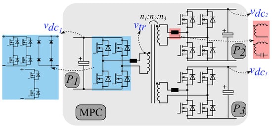
Figure 1. TAB DC–DC converter.

The main operational characteristic of this converter is its power flow control principle, which is achieved by controlling the phase difference between the three high-frequency AC voltages at each port, as shown in Figure 2a. The power flow is proportional to the phase difference between port voltages, and this simple power flow control is known as single phase shift. However, phase shifting pure square voltages induces high peak currents, which stress the semiconductors and increase losses. Therefore, other modulations such as dual and triple phase shifts (see Figure 2b,c) are used to reduce the peak currents, which increases the zero-voltage-switching range and reduces switching and conduction losses. These modulation strategies have little to no effect on the power flow [14,39]. Since this work focuses on modeling and control, the simplest modulation —single phase shift (SPS)— is considered for the rest of the analyses.

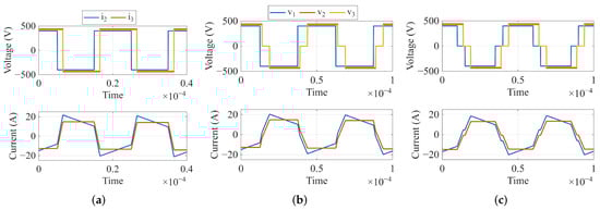
Figure 2. Modulation techniques for the TAB converter: (a) single phase shift, (b) dual phase shift, (c) triple phase shift.

3. Modeling of the TAB

In this section, the switching, generalized average full-order model, and average ROM are derived and compared.

The most generic and detailed model is the switching model. Here, the mathematical formalism of the switching behavior of the TAB operating under SPS is detailed first. Then, the first harmonic approximation is applied to describe the AC square voltages, and a generalized average model is presented. Finally, the generalized average model is reduced to represent the dynamic behavior of the DC components under power flow changes.

3.1. Switching Model

The switching model mathematically represents the square-wave voltages generated by the switching actions of the bridges’ semiconductors. Assuming that the DC link voltage at each port i is $v_{d{c}_i}$, the squared AC voltage applied to the transformer, $v_i^{ac}$, is represented by the product of a signed piece-wise function $S_i$ and the DC voltage, as shown in (1) and (2).

These voltages are phase shifted from each other by controlled angles ${\varphi }_1$, ${\varphi }_2$, and ${\varphi }_3$, thus allowing a controlled power flow.

$$S_i=\{\begin{array}{ll}1& 0+{\varphi }_i<\tau \le \pi +{\varphi }_i(S_{i_1},S_{i_4}ON)\\ -1& \pi +{\varphi }_i<\tau \le 2\pi +{\varphi }_i(S_{i_2},S_{i_3}ON)\end{array}$$

(1)

$$v_i^{ac}=S_i\left(t\right)·v_{d{c}_i}$$

(2)

Once the AC voltages are defined, the dynamic equation of the currents flowing in the reactive network $i_{L_i}$ can be derived by applying the Kirchhoff voltage law in the equivalent circuits depicted in Figure 3. These equivalent circuits are referred to the primary winding (Port 1) and assume an ideal transformer with magnetizing inductance $L_m>>L_i$. In this case, the $\Delta$-equivalent circuit referred to the primary winding is more convenient since it removes the transformer voltage from this expression. However, the Y-equivalent circuit can be more intuitive for some readers since it resembles the original circuit. Its equivalence leaves the choice to the convenience of the reader. Equations (3)–(5) represent the AC currents’ dynamic response for the $\Delta$ and Y equivalent models, respectively, assuming that equivalent currents flow between ports i and j, where $i,j\in \{1,2,3\}$ and $i\ne j$. The equivalent $\Delta$ impedance $Z_{ij}$ is derived from the Y-equivalent circuit using (6). Moreover, equivalent parasitic resistance $R_{s_i}$ is included to represent semiconductor conduction losses and Joule losses in the transformer windings. Finally, the dynamic response of the DC link capacitor voltages is represented in (7). Thus, considering the transformer leakage inductance currents $i_{Li}$ and the capacitor voltages $v_{d{c}_i}$ as state variables, the full-order switched model of the TAB is represented using Equations (4) and (7) for each port i. Without loss of generality, it is a common choice to select Port 1 as the reference port with ${\varphi }_1=0$ and a fixed $v_{d{c}_1}$. This assumption is used in this work.

$${\displaystyle \frac{d{i}_{L_{ij}}}{dt}}=-{\displaystyle \frac{R_{sij}}{L_{ij}}}{i}_{L_{ij}}+{\displaystyle \frac{v_{d{c}_i}}{L_{ij}}}{S}_i-{\displaystyle \frac{n_{ij}{v}_{d{c}_j}}{L_{ij}}}{S}_j,\forall i,j\in \{1,2,3\}$$

(3)

$${\displaystyle \frac{d{i}_{L_i}}{dt}}=-{\displaystyle \frac{R_{si}}{L_i}}{i}_{L_i}+{\displaystyle \frac{v_{d{c}_i}}{L_i}}{S}_i-{\displaystyle \frac{v_{tr}}{L_i}},\forall i\in \{1,2,3\}$$

(4)

$$i_{L_i}=i_{L_{i,j}}+i_{L_{i,k}},\forall i,j,k\in \{1,2,3\}\wedge i\ne j\wedge i\ne k.$$

(5)

$$Z_{i,j}=Z_i^{\prime }+Z_j^{\prime }+{\displaystyle \frac{Z_i^{\prime }{Z}_j^{\prime }}{Z_k^{\prime }}},\forall i,j,k\in \{1,2,3\}\wedge k\ne i,j$$

(6)

$${\displaystyle \frac{d{v}_{d{c}_i}}{dt}}={\displaystyle \frac{i_{d{c}_i}-i_{L_i}{S}_i}{C_i}}$$

(7)

where $n_{ij}={\displaystyle \frac{n_j}{n_i}}$ is the transformer turn ratio from Port j to Port i, $v_{tr}$ is the transformer voltage, and $Z_i^{\prime }$ is the leakage inductance at each Port i reflected to Port 1 ($Z_j^{\prime }=n_{1j}^2{Z}_j,\forall j\in \{2,3\}$).

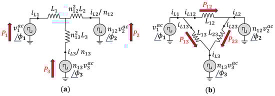
Figure 3. (a) Y-type primary-referred equivalent circuit. (b) $\Delta$-type primary-referred equivalent circuit.

3.2. Generalized Average Model

This subsection describes the mathematical model of the TAB obtained using the GAM [16]. This approach can be used to derive a mathematical representation of average signals in power converter topologies with AC signals, where the small-ripple approximation is not valid. Authors in [17,18] proposed GAM-based models of the TAB using the first harmonic approximation in Y and $\Delta$ equivalent circuits, respectively, to obtain both large- and small-signal models.

The GAM is based on a complex Fourier series representation of state variables in the interval $t-T\le \tau \le T$ as described in (8).

$$x\left(\tau \right)=\sum _k{x}_k\left(t\right)e^{jk{\omega }_s\tau }$$

(8)

$${⟨x⟩}_k\left(t\right)={\displaystyle \frac{1}{T}}{\int }_{t-T}^{T}x\left(\tau \right)e^{-jk{\omega }_s\tau }d\tau$$

(9)

where $x_k$ is the Fourier coefficient for each harmonic considered in the series representation, defined as in (9). This coefficient can be interpreted as a sliding average estimated at periodic intervals, and it is useful to represent the average of AC signals present in power converters.

When applying the GAM methodology in the TAB, two properties of Fourier coefficients are critical. First of all, the derivative of the sliding average is as in (10) and the product of variables, which results in the convolutional relationship shown in (11).

$${\displaystyle \frac{d{⟨x⟩}_k\left(t\right)}{dt}}={⟨{\displaystyle \frac{dx}{dt}}⟩}_k\left(t\right)-jk{\omega }_s{⟨x⟩}_k\left(t\right)$$

(10)

$${⟨xy⟩}_k\left(t\right)=\sum _i{⟨x⟩}_{k-i}{⟨y⟩}_i$$

(11)

To obtain a GAM of the TAB, only DC (subscript 0) and first harmonic approximation (FHA) (subscript 1) terms in the Fourier series are considered in this work. Hence, by applying the procedure described in [40] to the switching model described by (4) and (7), with the state variables $i_{L_i}$ and $v_{d{c}_i}$ of Ports 2 and 3, the GAM of the TAB converter considering the Y-equivalent circuit is presented in (12), with R and I subscripts indicating real and imaginary parts of the Fourier coefficients.

$$\begin{array}{cc}\hfill & {\displaystyle \frac{d}{dt}}{⟨v_{d{c}_i}⟩}_0=-{\displaystyle \frac{1}{C_i{R}_i}}{⟨v_{d{c}_i}⟩}_0-{\displaystyle \frac{1}{C_i}}{⟨S_i⟩}_{1R}{⟨i_{L_i}⟩}_{1R}-{\displaystyle \frac{1}{C_i}}{⟨S_i⟩}_{1I}{⟨i_{L_i}⟩}_{1I},\forall i\in \{2,3\}\hfill \\ \hfill & {\displaystyle \frac{d}{dt}}{⟨i_{L_i}⟩}_{1R}=-{\displaystyle \frac{R_{si}}{L_i}}{⟨i_{L_i}⟩}_{1R}+{\omega }_s{⟨i_{L_i}⟩}_{1I}+{\displaystyle \frac{{⟨S_i⟩}_{1R}}{L_i}}{⟨v_{d{c}_i}⟩}_0-{\displaystyle \frac{n_i}{L_i}}{⟨v_{tr}⟩}_{1R},\forall i\in \{2,3\}\hfill \\ \hfill & {\displaystyle \frac{d}{dt}}{⟨i_{L_i}⟩}_{1I}=-{\displaystyle \frac{R_{si}}{L_i}}{⟨i_{L_i}⟩}_{1I}-{\omega }_s{⟨i_{L_i}⟩}_{1R}+{\displaystyle \frac{{⟨S_i⟩}_{1I}}{L_i}}{⟨v_{d{c}_i}⟩}_0-{\displaystyle \frac{n_i}{L_i}}{⟨v_{tr}⟩}_{1I},\forall i\in \{2,3\}\hfill \end{array}$$

(12)

The Fourier coefficients of the SPS modulation switching functions $S_i$ are presented in (13). Moreover, an expression for the transformer windings’ voltage $v_{tr}$ is derived using the principle of superposition, assuming a linear behavior in the transformer, leaving the expression presented in (14). The equivalent impedance expression are presented in Equations (A1) and (A2).

$$\begin{array}{cccccc}\hfill & {⟨S_1⟩}_{1R}=0\hfill & \hfill & {⟨S_1⟩}_{1I}=-{\displaystyle \frac{2}{\pi }}\hfill & \hfill & {⟨S_2⟩}_{1R}=-{\displaystyle \frac{2sin{\varphi }_{12}}{\pi }}\hfill \\ \hfill & {⟨S_2⟩}_{1I}=-{\displaystyle \frac{2cos{\varphi }_{12}}{\pi }}\hfill & \hfill & {⟨S_3⟩}_{1R}=-{\displaystyle \frac{2sin{\varphi }_{13}}{\pi }}\hfill & \hfill & {⟨S_3⟩}_{1I}=-{\displaystyle \frac{2cos{\varphi }_{13}}{\pi }}\hfill \end{array}$$

(13)

$$\begin{array}{cc}\hfill & {⟨v_{tr}⟩}_1={\displaystyle \frac{2\Im \left\{Z_{eq,2}\right\}}{\pi }}{V}_1+{\displaystyle \frac{2}{\pi }}\left(\Im \left\{Z_{eq,3}\right\}cos{\varphi }_{12}-\Re \left\{Z_{eq,3}\right\}sin{\varphi }_{12}\right){\displaystyle \frac{{⟨v_{d{c}_2}⟩}_0}{n_2}}\hfill \\ & +{\displaystyle \frac{2}{\pi }}\left(\Im \left\{Z_{eq,1}\right\}cos{\varphi }_{13}-\Re \left\{Z_{eq,1}\right\}sin{\varphi }_{13}\right){\displaystyle \frac{{⟨v_{d{c}_3}⟩}_0}{n_3}}\hfill \\ \hfill & {⟨v_{tr}⟩}_{1I}=-{\displaystyle \frac{2\Re \left\{Z_{eq,2}\right\}}{\pi }}{V}_1-{\displaystyle \frac{2}{\pi }}\left(\Re \left\{Z_{eq,3}\right\}cos{\varphi }_{12}+\Im \left\{Z_{eq,3}\right\}sin{\varphi }_{12}\right){\displaystyle \frac{{⟨v_{d{c}_2}⟩}_0}{n_2}}\hfill \\ & -{\displaystyle \frac{2}{\pi }}\left(\Re \left\{Z_{eq,1}\right\}cos{\varphi }_{13}+\Im \left\{Z_{eq,1}\right\}sin{\varphi }_{13}\right){\displaystyle \frac{{⟨v_{d{c}_3}⟩}_0}{n_3}}\hfill \end{array}$$

(14)

Finally, substituting (13) and (14) in (12), the system of equations representing the TAB large-signal model is shown as a state space equation in (15), where brackets and subscripts 0 and 1 (DC variables and FHA) were removed, and the coefficients $a_i$ with $i\in \{1,\dots ,8\}$ are presented in Equation (A3). Readers can refer to [17,18] for a more detailed derivation.

$$\left[\begin{array}{c}{\dot{v}}_{d{c}_2}\\ {\dot{v}}_{d{c}_3}\\ {\dot{i}}_{L_{2}R}\\ {\dot{i}}_{L_{2}I}\\ {\dot{i}}_{L_{3}R}\\ {\dot{i}}_{L_{3}I}\end{array}\right]=\left[\begin{array}{cccccc}-{\displaystyle \frac{1}{C_2{R}_2}}& 0& {\displaystyle \frac{4sin{\varphi }_{12}}{\pi C_2}}& {\displaystyle \frac{4cos{\varphi }_{12}}{\pi C_2}}& 0& 0\\ 0& -{\displaystyle \frac{1}{C_3{R}_3}}& 0& 0& {\displaystyle \frac{4sin{\varphi }_{13}}{\pi C_3}}& {\displaystyle \frac{4cos{\varphi }_{13}}{\pi C_3}}\\ a_1& a_2& -{\displaystyle \frac{R_{s2}}{L_2}}& {\omega }_s& 0& 0\\ a_3& a_4& -{\omega }_s& -{\displaystyle \frac{-R_{s2}}{L_2}}& 0& 0\\ a_5& a_6& 0& 0& -{\displaystyle \frac{R_{s3}}{L_3}}& {\omega }_s\\ a_7& a_8& 0& 0& -{\omega }_S& -{\displaystyle \frac{R_{s3}}{L_3}}\end{array}\right]\left[\begin{array}{c}{v}_{d{c}_2}\\ v_{d{c}_3}\\ i_{L_{2}R}\\ i_{L_{2}I}\\ i_{L_{3}R}\\ i_{L_{3}I}\end{array}\right]+\left[\begin{array}{c}0\\ 0\\ -{\displaystyle \frac{2n_{1,2}}{\pi L_2}}\\ {\displaystyle \frac{2n_{1,2}}{\pi L_2}}\\ -{\displaystyle \frac{2n_{1,3}}{\pi L_3}}\\ -{\displaystyle \frac{2n_{1,3}}{\pi L_3}}\end{array}\right]V_1$$

(15)

3.3. Reduced-Order Model

This subsection presents a ROM for the TAB, which neglects the fast dynamics of the high-frequency transformer currents and focuses on slower dynamics in the output capacitors’ voltage. The same modulation assumptions made for the GAM are valid in this case. Furthermore, assuming a linear behavior in the transformer, as in the GAM, the principle of superposition can also be used for the power flow. Thus, the power flow equations derived for the dual active bridge can be used to represent the power flowing between each pair of ports as in (16). The reader can refer to [41] for the dual active bridge power flow mathematical model, which facilitates understanding of the modeling principles applied and described in this section. The total power delivered or absorbed by each port is presented in (17). Moreover, the current at each port is computed by simply dividing the power by the voltage as in (18). Hence, the operation of the TAB can be simplified to a first-order system where the output capacitor voltages are the state variables as presented in (19). A graphical representation of the TAB circuit and its average ROMs is presented in Figure 4, where $C_{d{c}_1}$ is the input capacitor and is considered sufficiently high so that port 1 can be treated as a constant DC voltage.

$$P_{ij}=-P_{ji}={\displaystyle \frac{n_{ij}{v}_{d{c}_i}{v}_{d{c}_j}{\varphi }_{ij}(1-\frac{|{\varphi }_{ij}|}{\pi })}{{\omega }_{sw}{L}_{ij}}},\forall i,j\in \{1,2,3\}\wedge i\ne j.$$

(16)

$$P_i=\sum _{\begin{array}{c}j=1\\ j\ne i\end{array}}^3{P}_{ij},\forall i\in \{1,2,3\}$$

(17)

$$i_i={\displaystyle \frac{P_i}{v_{d{c}_i}}}=\sum _{\begin{array}{c}j=1\\ j\ne i\end{array}}^3{\displaystyle \frac{n_{ij}{v}_{d{c}_j}{\varphi }_{ij}(1-\frac{|{\varphi }_{ij}|}{\pi })}{{\omega }_{sw}{L}_{ij}}},\forall i\in \{2,3\}$$

(18)

$$\begin{array}{c}\hfill {\displaystyle \frac{d{v}_{d{c}_i}}{dt}}={\displaystyle \frac{i_{d{c}_i}-i_i}{C_i}},\forall i\in \{2,3\}\end{array}$$

(19)

where ${\varphi }_{ij}=-{\varphi }_{ji}={\varphi }_j-{\varphi }_i$ is the phase shift between Ports i and j, $n_{ij}$ is the turns ratio between port windings in the high-frequency transformer, $v_{d{c}_i}$ and $v_{d{c}_j}$ are the voltages at Ports i and j, ${\omega }_{sw}$ is the switching frequency of the active bridges, $L_{ij}$ are the equivalent inductance between Ports i and j, and $C_i$ is the capacitance at Port i.

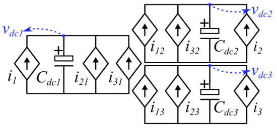
Figure 4. TAB reduced-order model.

Another alternative for the ROM is to describe the power flow based on the FHA instead of the square waveforms. The FHA provides a straightforward procedure to derive the power flow equation based on the lossless transmission power systems equations [42]. For this, the fundamental component of a squared voltage is represented by the Fourier coefficient (20).

$$V_{FHA,i}={\displaystyle \frac{4V_{d{c}_i}}{\pi \sqrt{2}}}$$

(20)

Therefore, the power flow between two ports ($i,j$) connected through the transformer can be approximated as two sinusoidal voltage sources connected through an inductor and use the power equation as presented in (21)–(27). Hence, FHA power flow equations can be used in (19) to obtain an alternative version of the TAB ROM.

$$S_{FH{A}_{i,j}}=V_{FHA,i}{I}_{FH{A}_{i,j}}^{\ast }$$

(21)

$$I_{FH{A}_{ij}}={\displaystyle \frac{V_{FHA,i}\angle 0^{\circ }-n_{i,j}{V}_{FHA,j}\angle {\varphi }_{ij}}{j{X}_{ij}}}$$

(22)

$$I_{FH{A}_{ij}}=-{\displaystyle \frac{n_{ij}{V}_{FHA,j}sin\left({\varphi }_{ij}\right)}{X_{ij}}}+j{\displaystyle \frac{n_{i,j}{V}_{FHA,j}cos\left({\varphi }_{ij}\right)-V_{FHA,i}}{X_{ij}}}$$

(23)

$$P_{FH{A}_{ij}}=\Re \left\{S_{FH{A}_{ij}}\right\}={\displaystyle \frac{v_{FH{A}_i}{n}_{ij}{v}_{FH{A}_j}sin{\varphi }_{ij}}{X_{ij}}}=V_{FH{A}_i}\Re \left\{I_{FH{A}_{ij}}\right\}$$

(24)

$$P_{FH{A}_{ij}}={\displaystyle \frac{8}{{\pi }^2}}{\displaystyle \frac{v_{d{c}_i}{n}_{i,j}{v}_{d{c}_j}}{\omega L_{ij}}}sin{\varphi }_{ij}$$

(25)

$$Q_{FH{A}_{ij}}=\Im \left\{S_{FH{A}_{ij}}\right\}={\displaystyle \frac{v_{FH{A}_i}{n}_{i,j}{v}_{FHA,j}cos\left({\varphi }_{ij}\right)-V_{FHA,i}^2}{X_{ij}}}=V_{FH{A}_i}\Im \left\{I_{FH{A}_{ij}}\right\}$$

(26)

$$Q_{FH{A}_{ij}}={\displaystyle \frac{8}{{\pi }^2}}{\displaystyle \frac{v_{d{c}_i}{n}_{i,j}{v}_{d{c}_j}cos{\varphi }_{ij}-v_{d{c}_i}^2}{\omega L_{ij}}}$$

(27)

3.4. Model Comparison

In Section 3, three different models are presented. Here, the models are compared considering the switching model as the reference. The models are built in Simulink using the Simscape toolbox for switching circuits. Continuous state-space and dynamic blocks are used for the GAM and ROMs. A good compromise between accuracy and model complexity can be achieved by considering only the first-order harmonic [40]. However, steady-state errors could be considerable for certain operational conditions [43]. Here, the steady-state error and dynamic representation are evaluated for the GAM and ROM. For the ROMs, only the one based on the squared waveforms is considered.

Figure 5, Figure 6 and Figure 7 show the steady-state output voltages and their error with respect to the switching model in open-loop operation for several phase shift combinations. The case where ${\varphi }_{12}={\varphi }_{13}$ is presented in Figure 5, where the ROM seems to represent the output voltage slightly better than the GAM, and both models have a similar tendency to reduce the error as the phase shift increases. However, when ${\varphi }_{12}\ne {\varphi }_{13}$ (Figure 6 and Figure 7), the conclusion is not as obvious as in the previous case. When ${\varphi }_{12}\ne {\varphi }_{13}$, the power flow coupling between Ports 2 and 3 strengthens, and when ${\varphi }_{12}$ increases, $v_{d{c}_2}$ and $v_{d{c}_3}$ error behavior is inverse for the GAM and the ROM, and the best representation is highly dependent on the operating point. Furthermore, when the time-domain response is analyzed, the GAM represents some dynamics that the ROM cannot. Figure 8 and Figure 9 show the time domain comparison of the models in open-loop operation, with constant and equal phase shift for two different operating points, and two load disturbances in Ports 2 and 3 at t = 2 s and t = 4 s, respectively. The zoomed visualization shows how the ROM cannot represent the impact of Port 2 disturbances on Port 3, and vice versa. On the other hand, the GAM model can represent this coupling, which is an important aspect in the TAB dynamic response. However, when the phase shift between Port 2 and Port 3 increases, the ROM can represent the coupling. This can be explained by the lossless assumption made in the ROM, which ignores the power flow due to the resistor in the reactive network of each port. This can be represented better by the GAM. However, the power flow is better represented by the ROM due to the phase shift effect, and the GAM power flow is underestimated due to the first harmonic limitation.

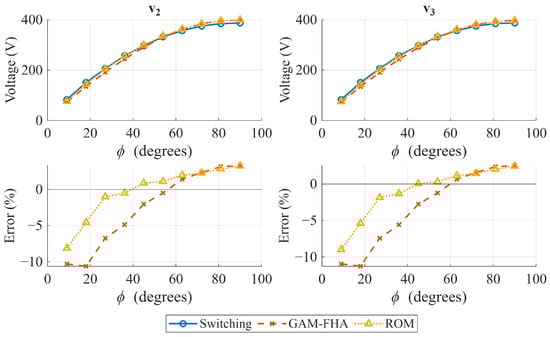
Figure 5. Open-loop operation comparison. Steady-state values of output voltages $v_{d{c}_2}$ and $v_{d{c}_3}$. ${\varphi }_{12}$ = ${\varphi }_{13}$.

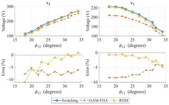
Figure 6. Open-loop operation comparison. Steady-state values of output voltages $v_{d{c}_2}$ and $v_{d{c}_3}$. ${\varphi }_{13}$ = 27°, ${\varphi }_{12}\in$ [18°,34°].

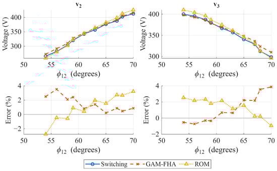
Figure 7. Open-loop operation comparison. Steady-state values of output voltages $v_{d{c}_2}$ and $v_{d{c}_3}$. ${\varphi }_{13}$ = 36°, ${\varphi }_{12}\in$ [54°,70°].

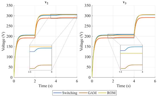
Figure 8. Open-loop operation comparison. Steady-state values of output voltages $v_{d{c}_2}$ and $v_{d{c}_3}$. ${\varphi }_{12}={\varphi }_{13}$ = 27°.

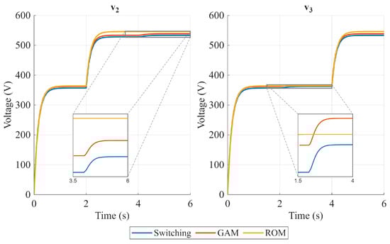
Figure 9. Open-loop operation comparison. Steady-state values of output voltages $v_{d{c}_2}$ and $v_{d{c}_3}$. ${\varphi }_{12}={\varphi }_{13}$ = 63°.

Including more harmonic components in the GAM could improve the power flow representation at the cost of higher complexity and computational burden. Furthermore, both models can be used to represent a specific operating point if parameters are selected correctly. Therefore, linearized models derived from the GAM or the ROM can be used to design a linear controller, as explored in the next section. Furthermore, a ROM can be the closest representation for nonlinear controllers. Table 1 summarizes the main aspects of the model comparison, including assumptions made, main advantages and drawbacks, and where to use each model.

Table 1. Model comparison summary.

	Switching	GAM	ROM
Assumptions	-	Full-order model ($v_{d{c}_i}$ and $i_{L_i}$), FHA for AC signals and power flow estimation, losses represented by $R_{si}$, SPS modulation	Reduced-order model (only $v_{d{c}_i}$), $i_{L_i}$ dynamics neglected, lossless power flow based on full-harmonic content, SPS modulation
Advantages	Closest to reality	Port coupling, losses, and AC dynamic representation	Better trade-off between complexity and accuracy
Drawbacks	Computational burden	Higher complexity, limited power flow	Limited port coupling
Application	Modulation studies, soft-switching studies, model validation	Small-signal stability analysis, linear controller design, feedforward controller design	Linear and nonlinear controller design

4. Control Strategy

The TAB converter is a nonlinear and magnetically coupled system. This coupling causes the power supplied through the converter ports to be interdependent, as shown in (17). Figure 10 illustrates the coupled power flow effect when the control variables ${\varphi }_{12}$ and ${\varphi }_{13}$ vary independently. Consequently, designing a controller that ensures decoupled power flow, stability, and efficient power sharing is a major challenge.

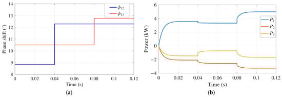
Figure 10. Coupled power flow in TAB: (a) ports 2 and 3 phase shift, (b) power at each port.

This section presents the design of three decoupling power flow control strategies for the TAB converter, whose focus is on voltage control. The strategies include inverse matrix decoupling (IDM), a linear active disturbance rejection (LADR) controller, and a sliding mode controller (SMC) based on a linear extended state observer (LESO). The mathematical foundations of each strategy are presented for the TAB converter case, improving the ease of replicability. For the control design, the TAB Ports 2 and 3 are considered as load ports connected to rated resistances $R_{load,2}$ and $R_{load,3}$, respectively.

4.1. Inverse Decoupling Matrix

This first strategy is based on an IDM, which is designed to mitigate or eliminate the coupling in the TAB converter, transforming it into two fictitious decoupled subsystems that can be controlled using traditional PI controllers. The next subsections detail the PI controller and the IDM design.

4.1.1. PI Control

The design of the PI controller can be based on a linearized model of the GAM model or the ROM. In this work, the PI is designed considering a linearized version of the GAM presented in (15). The linearized small-signal model is presented in Equation (A4), and a more detailed derivation can be found in [17,22]. The controller presented here computes the manipulated variables ${\varphi }_{1,2}$ and ${\varphi }_{1,3}$ using independent PI controllers for the voltage control of Ports 2 and 3, assuming port decoupling.

For the derivation of the PI gains, the differential equation presented in (28) that represents the change in the output port voltages $\Delta v_{d{c}_j}\forall j\in \{2,3\}$ is considered.

$$C_j{\displaystyle \frac{d\Delta v_{d{c}_j}\left(t\right)}{dt}}=-{\displaystyle \frac{\Delta v_{d{c}_j}\left(t\right)}{R_j}}-\Delta i_{d{c}_j}\left(t\right)+{\displaystyle \frac{4}{\pi }}\left(\Delta i_{L_{j}R}\left(t\right)sin\left({\varphi }_{1j}\right)+\Delta i_{L_{j}I}\left(t\right)cos\left({\varphi }_{1j}\right)\right)+{\displaystyle \frac{4}{\pi }}{I}_{L_j}\Delta {\varphi }_{1j}\left(t\right)$$

(28)

where $I_{L_j}=I_{L_{j}R}cos\left({\varphi }_{1j}\right)-I_{L_{j}I}sin\left({\varphi }_{1j}\right)$.

By applying some algebraic transformation over (28), the resulting expression isolates the manipulated variable $\Delta {\varphi }_{1,j}$ as in (29). Assuming no load and transformer currents disturbances, (28) can be simplified as in (30) where the voltage dynamic depends only on the manipulated variable ${\varphi }_{1,j}$.

$${\displaystyle \frac{\pi C_j}{4I_{L_j}}}{\displaystyle \frac{d\Delta v_{d{c}_j}\left(t\right)}{dt}}=-{\displaystyle \frac{\pi \Delta v_{d{c}_j}\left(t\right)}{4I_{L_j}{R}_j}}-{\displaystyle \frac{\pi \Delta i_{d{c}_j}\left(t\right)}{4I_{L_j}}}+{\displaystyle \frac{\left(\Delta i_{L_{j}R}\left(t\right)sin\left({\varphi }_{1j}\right)+\Delta i_{L_{j}I}\left(t\right)cos\left({\varphi }_{1j}\right)\right)}{I_{L_j}}}+\Delta {\varphi }_{1j}\left(t\right)$$

(29)

$${\displaystyle \frac{\pi C_j}{4I_{L_j}}}{\displaystyle \frac{d\Delta v_{d{c}_j}\left(t\right)}{dt}}+{\displaystyle \frac{\pi \Delta v_{d{c}_j}\left(t\right)}{4I_{L_j}{R}_j}}=\Delta {\varphi }_{1j}\left(t\right)$$

(30)

Then, the Laplace transformation is applied to (30) and a simplified plant transfer function (31) is obtained. The transfer function is used to design a PI controller applying the pole placement method,

$${\displaystyle \frac{\Delta v_{d{c}_j}\left(s\right)}{\Delta {\varphi }_{1j}^{FB}\left(s\right)}}={\displaystyle \frac{\frac{4}{\pi }(I_{L_{j}R}cos\left({\varphi }_{1j}\right)-I_{L_{j}I}sin\left({\varphi }_{1j}\right))}{s+{\tau }_j}}$$

(31)

where ${\tau }_j={\displaystyle \frac{1}{C_j{R}_j}}$.

Considering (31), the PI controller can be designed with the controller gains as in (32) and (33).

$$k_p={\displaystyle \frac{2\xi {\omega }_n-{\tau }_j}{\frac{4}{\pi C_j}(I_{L_{j}R}cos\left({\varphi }_{1j}\right)-I_{L_{j}I}sin\left({\varphi }_{1j}\right))}}$$

(32)

$$k_i={\displaystyle \frac{{\omega }_n^2}{\frac{4}{\pi C_j}(I_{L_{j}R}cos\left({\varphi }_{1j}\right)-I_{L_{j}I}sin\left({\varphi }_{1j}\right))}}$$

(33)

4.1.2. IDM Design

The inverse decoupling matrix (IDM) aims to transform the coupled MIMO system into a set of independent SISO systems, where each output is influenced only by its corresponding input. It simplifies controller design by allowing a controller to be designed for each subsystem independently of the others. The IDM is designed using the linearized small-signal transfer function matrix, G, of the TAB [21,24,25,44]. To obtain G, the port currents and phase shift angles in (18) are expressed as their DC operating point values plus small perturbation values. By neglecting second-order nonlinear terms over a switching period, G is derived as

$$\left(\begin{array}{c}\Delta i_2\\ \Delta i_3\end{array}\right)=G\left(\begin{array}{c}\Delta {\varphi }_{12}\\ \Delta {\varphi }_{13}\end{array}\right)=\left(\begin{array}{cc}{g}_{22}& g_{23}\\ g_{32}& g_{33}\end{array}\right)\left(\begin{array}{c}\Delta {\varphi }_{12}\\ \Delta {\varphi }_{13}\end{array}\right)$$

(34)

with

$$g_{ii}=\{\begin{array}{ll}-{\sum }_{\begin{array}{c}k=1\\ k\ne i\end{array}}^3{\displaystyle \frac{n_{Ki}{V}_{d{c}_k}(1-2\frac{|{\Phi }_{ki}|}{\pi })}{{\omega }_{sw}{L}_{ki}}},& \forall i,j\in \{2,3\}\wedge i=j.\\ {\displaystyle \frac{n_{ji}{V}_{dcj}}{{\omega }_s{L}_{ij}}}(1-2{\displaystyle \frac{|{\Phi }_{ij}|}{\pi }}),& \forall i,j\in \{2,3\}\wedge i\ne j.\end{array}$$

(35)

where $V_{d{c}_i}$ and ${\Phi }_{ij}$ are DC components of DC voltage at Port i and phase shift, respectively.

To ensure a decoupled power flow, the IDM H is obtained as the inverse of the gain matrix G, as in (36). To implement this strategy, the elements of H should be precomputed alongside the optimum operating points and stored in corresponding lookup tables.

$$H=G^{-1}=\left[\begin{array}{cc}{h}_{22}& h_{23}\\ h_{32}& h_{33}\end{array}\right]$$

(36)

Figure 11 depicts the block diagram of the decoupled matrix controller applied in the TAB converter. $H_{LPF,v_i}$ is the low-pass filter transfer function, which yields the voltage $v_{d{c}_i}$ as defined in (37).

$$\begin{array}{cc}\hfill & H_{LPF,v_i}={\displaystyle \frac{R_{load,i}}{R_{load,i}{C}_{i}s+1}},i\in \{2,3\}\hfill \end{array}$$

(37)

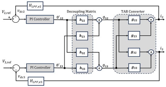
Figure 11. Block diagram of TAB converter model and the decoupling network.

From Figure 11, one can deduct that Equation (34) can be reformulated as follows:

$$\left(\begin{array}{c}\Delta i_2\\ \Delta i_3\end{array}\right)=GH\left(\begin{array}{c}\Delta {\varphi }_{12}^{\prime }\\ \Delta {\varphi }_{13}^{\prime }\end{array}\right)$$

(38)

According to (38), each SISO system depends on one auxiliary variable, either ${\varphi }_{12}^{\prime }$ or ${\varphi }_{13}^{\prime }$. Therefore, a basic PI controller is sufficient for each one.

It is worth mentioning that while the IDM strategy successfully decomposes the TAB converter into independent SISO systems, their practical application is constrained by several limitations, including high computational burden and sensitivity to operating point variations and model uncertainties.

4.2. Linear Active Disturbance Rejection Control

Linear active disturbance rejection control (LARDC) [45,46,47] is a control technique that aims to reduce the impact of disturbances in the plant. Unlike conventional control methods, LADRC depends only on the system’s order, does not require an accurate mathematical model, and is relatively simple to implement. These attributes have contributed to its broad applications [48,49,50,51,52]. Figure 12 shows the functional block diagram of the LADRC. As can be seen, ADRC consists of three elements: a trajectory differentiator (TD), a linear extended state observer (ESO), and a controller. The TD takes as input the reference signal and generates its derivatives. The ESO is the core of LADRC, as it estimates all system states, along with disturbances (both internal and external), which enables disturbance compensation in the control strategy. By compensating for this estimated disturbance in real time, the ESO significantly enhances the system’s robustness and reliability. Finally, the controller generates a control signal that is designed under the assumption that the plant has been modified to behave like a desired, disturbance-free nominal system.

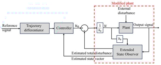
Figure 12. Functional block diagram of LADRC.

The design of the LADRC controller is based on the ROM presented in (19), which is a nonlinear model, unlike the one proposed that uses the small-signal model, potentially impacting its efficiency when the operating point is changed. Before approaching the LADRC controller design process for each port of the TAB, we consider an auxiliary control variable $u_i$ defined as

$$\begin{array}{c}\hfill u_i={\varphi }_{1i}(1-{\displaystyle \frac{|{\varphi }_{1i}|}{\pi }}),\forall i\in \{2,3\}\end{array}$$

(39)

where ${\varphi }_{1i}$ is given by

$${\varphi }_{1i}=\{\begin{array}{cc}{\displaystyle \frac{\pi }{2}}(1-\sqrt{1-{\displaystyle \frac{4u_i}{\pi }}}),& 0\le u_i<{\displaystyle \frac{\pi }{4}}\\ -{\displaystyle \frac{\pi }{2}}(1-\sqrt{1+{\displaystyle \frac{4u_i}{\pi }}}),& -{\displaystyle \frac{\pi }{4}}\le u_i<0\end{array}$$

(40)

The TAB ROM (19) can be rewritten as

$$\begin{array}{c}\hfill {\displaystyle \frac{d{v}_{d{c}_i}}{dt}}={\displaystyle \frac{n_{1i}{v}_{d{c}_1}}{{\omega }_{sw}{L}_{ij}{C}_i}}{u}_i-{\displaystyle \frac{n_{ij}{v}_{d{c}_j}{\varphi }_{ij}(1-\frac{|{\varphi }_{ij}|}{\pi })}{{\omega }_{sw}{L}_{ij}{C}_i}}-{\displaystyle \frac{i_{d{c}_i}}{C_i}},\forall i,j\in \{2,3\}\wedge i\ne j.\end{array}$$

(41)

Equation (41) describes the dynamics of a first-order SISO system and can be written in the following form:

$$\begin{array}{c}\hfill {\dot{y}}_i=b_{0,i}{u}_i+{\xi }_i(t,y,{\xi }_{ext}),\forall i\in \{2,3\}\end{array}$$

(42)

where $u_i$ is the control variable, $y=v_{d{c}_i}$ is the output to be controlled, $b_{0i}={\displaystyle \frac{n_{1i}{v}_{d{c}_1}}{{\omega }_{sw}{L}_{ij}{C}_i}}$ is the critical gain, and ${\xi }_i=-{\displaystyle \frac{n_{ij}{v}_{d{c}_j}{\varphi }_{ij}(1-\frac{|{\varphi }_{ij}|}{\pi })}{{\omega }_{sw}{L}_{ij}{C}_i}}+{\displaystyle \frac{i_{d{c}_i}}{C_i}}$ is the total disturbance, which is defined as the combination of coupling effect and external disturbances ${\xi }_{ext}$.

Assuming that ${\xi }_i$ is differentiable and its derivative ${\dot{\xi }}_i$ is bounded, (42) can be rewritten in an augmented state representation form as follows:

$$\{\begin{array}{c}{\dot{x}}_1=b_{0i}{u}_i+x_2\hfill \\ {\dot{x}}_2={\dot{\xi }}_i\hfill \\ y_i=x_1\hfill \end{array}$$

(43)

where $x_2={\xi }_i$ is the augmented state variable that represents the total disturbance. Equation (43) can be rewritten in the following matrix form:

$$\{\begin{array}{c}\dot{x}=Ax+B_i{u}_i+E{\dot{\xi }}_i\hfill \\ y_i=Cx\hfill \end{array}$$

(44)

where $x={\left[\begin{array}{cc}{x}_1& x_2\end{array}\right]}^T$ is the augmented state vector and $A=\left[\begin{array}{cc}0& 1\\ 0& 0\end{array}\right]$, $B_i={\left[\begin{array}{cc}0& b_{0,i}\end{array}\right]}^T$, $E={\left[\begin{array}{cc}0& 1\end{array}\right]}^T$, and $C=\left[\begin{array}{cc}1& 0\end{array}\right]$ are the state space representation matrices.

4.2.1. Design of Linear Extended State Observer

The ESO takes $u_i$ and $y_i$ as inputs and estimates the state vector and total disturbance. The linear version (LESO) is a Luenberger observer, and it is designed in the following matrix form:

$$\{\begin{array}{c}\dot{z}=Az+B_i{u}_i+{\Lambda }_i{e}_i\hfill \\ \widehat{y_i}=Cz\hfill \end{array}$$

(45)

where $z={\left[\begin{array}{cc}{z}_1& z_2\end{array}\right]}^T$ is the estimation of state vector x, ${\Lambda }_i={\left[\begin{array}{cc}{\lambda }_{1i}& {\lambda }_{2i}\end{array}\right]}^T$ is the observer gain, and $e_i=y_i-z_1$ is the the estimation error.

Subtracting (45) from (44), the dynamic behavior of the estimation error is described by (46).

$$\begin{array}{c}\hfill \dot{e}I=(A-L_{i}C)e_i+E{\dot{\xi }}_i\end{array}$$

(46)

The observer gains are tuned using the bandwidth parameterization method [53], which places all poles at the position $-{\omega }_{o,i}$ as in (47).

$$\begin{array}{c}\hfill det(sI-[A-L_{i}C])={(s+{\omega }_{oi})}^2\end{array}$$

(47)

Solving (47), the observer gains are obtained as

$$\begin{array}{c}\hfill {\lambda }_{1i}=2{\omega }_{oi},{\lambda }_{2i}={\omega }_{oi}^2\end{array}$$

(48)

where ${\omega }_{oi}$ is the observer bandwidth for each TAB port i in this case. A higher value of ${\omega }_{oi}$ results in a faster observer response and good estimation and rejection of the total disturbance. However, in practice, the achievable bandwidth is limited by sensor noise [54].

4.2.2. Design of Control Law

The controller is designed to reduce steady-state error and achieve the desired dynamic response. It generates a control signal that assumes that output ports are effectively decoupled, and the converter behaves as a disturbance-free nominal system. To achieve an active disturbance rejection, the total disturbance (${\widehat{\xi }}_i=z_2$), estimated by LESO, is subtracted from the control law $u_{0i}$ generated by the controller. From Figure 12, the control law is designed as in (49).

$$\begin{array}{c}\hfill u_i={\displaystyle \frac{u_{0i}-{\widehat{\xi }}_i}{b_{0i}}}\end{array}$$

(49)

Assuming that the gains of LESO are well tuned ($y_i\approx z_1$ and ${\xi }_i\approx {\widehat{\xi }}_i\approx z_2$) and substituting (49) into (42), the system becomes as in (50).

$$\begin{array}{c}\hfill {\dot{y}}_i=u_{0i}\end{array}$$

(50)

It can be seen that the system becomes a single integrator free from disturbances, which can be controlled as follows:

$$\begin{array}{c}\hfill u_{0,i}=K_{p_i}(V_{i,\mathrm{ref}}-z_1)\end{array}$$

(51)

where $V_{i,\mathrm{ref}}$ is the reference output voltage and $K_{p_i}$ is the controller gain.

Using the bandwidth parameterization method, as in the observer design, the controller gain is tuned so that the pole is located at $-{\omega }_{ci}$ (52),

$$\begin{array}{c}\hfill K_{p_i}={\omega }_{ci}\end{array}$$

(52)

where ${\omega }_{ci}$ is the controller bandwidth of each TAB Port i, which is assumed to be a SISO system.

The LADRC block diagram for the TAB converter is shown in Figure 13.

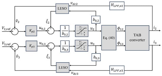
Figure 13. LADRC block diagram for the TAB converter.

4.2.3. Impact of the Controller and Observer Bandwidths

The above mathematical analysis shows that LADRC’s performance and closed-loop stability depend on the observer and controller bandwidths, $w_{oi}$ and $w_{ci}$, respectively. Therefore, the impact of those bandwidths on the controller stability and performance is investigated using frequency-domain analysis. The s-domain expressions for $z_1$ and $z_2$ are derived by substituting (49) into (45) and applying the Laplace transformation, as given below:

$$\begin{array}{cc}\hfill & Z_1\left(s\right)={\displaystyle \frac{2w_{oi}}{s+2w_{oi}+w_{ci}}}{Y}_i\left(s\right)+{\displaystyle \frac{w_{ci}}{s+2w_{oi}+w_{ci}}}{V}_{i,\mathrm{ref}}\hfill \\ \hfill & Z_2\left(s\right)={\displaystyle \frac{w_{oi}^2(s+w_{ci})}{s(s+2w_{oi}+w_{ci})}}{Y}_i\left(s\right)-{\displaystyle \frac{w_{oi}^2{w}_{ci}}{s(s+2w_{oi}+w_{ci})}}{V}_{i,\mathrm{ref}}\hfill \end{array}$$

(53)

Then, the ADRC control law (49) can be expressed as follows:

$$\begin{array}{cc}\hfill & U_i\left(s\right)=H_{V-u}\left(s\right)V_{i,\mathrm{ref}}-H_{y-u}\left(s\right)Y_i\left(s\right)\hfill \end{array}$$

(54)

where

$$\begin{array}{cc}\hfill & H_{V-u}\left(s\right)={\displaystyle \frac{1}{b_{0,i}}}{\displaystyle \frac{w_{ci}(s^2+2w_{oi}s+w_{oi}^2)}{s(s+2w_{oi}+w_{ci})}}\hfill \\ \hfill & H_{y-u}\left(s\right)={\displaystyle \frac{1}{b_{0,i}}}{\displaystyle \frac{(2w_{ci}{w}_{oi}+w_{oi}^2)s+w_{oi}^2{w}_{ci}}{s(s+2w_{oi}+w_{ci})}}\hfill \end{array}$$

Finally, combining (54) and (42), the output signal in the s-domain is as

$$\begin{array}{cc}\hfill & Y_i\left(s\right)=H_{V-y}\left(s\right)V_{i,\mathrm{ref}}\left(s\right)+H_{\xi -y}\left(s\right)\Xi \left(s\right)\hfill \end{array}$$

(55)

where

$$\begin{array}{cc}\hfill & H_{V-y}\left(s\right)={\displaystyle \frac{w_{ci}}{s+w_{ci}}}\hfill \\ \hfill & H_{\xi -y}\left(s\right)={\displaystyle \frac{s(s+2w_{oi}+w_{ci})}{(s+w_{ci})(s^2+2w_{oi}s+w_{oi}^2)}}\hfill \end{array}$$

As shown in (55), the output signal comprises a reference tracking term and a total disturbance term. Neglecting the total disturbance $\Xi \left(s\right)$ simplifies the output signal, demonstrating that tracking performance is governed by the control bandwidth ${\omega }_{ci}$. Figure 14 corroborates this relationship, showing that a higher ${\omega }_{ci}$ increases the stability margin and accelerates the tracking speed.

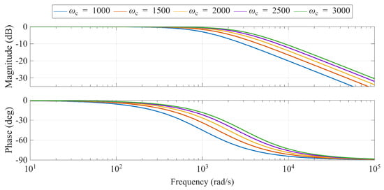
Figure 14. Bode diagram of $H_{V-y}\left(s\right)$ by varying the control bandwidth ${\omega }_{ci}$ (${\omega }_{oi}={10}^4$ rad/s).

$H_{V-y}\left(s\right)$ When considering the total disturbance $\Xi \left(s\right)$, the disturbance rejection capability is determined by $w_{ci}$ and $w_{oi}$. As shown in Figure 15 and Figure 16, increasing either $w_{oi}$ or $w_{ci}$ enhances this capability. Critically, $w_{oi}$ must be set higher than $w_{ci}$ to ensure the state estimates are accurate enough for the controller to function correctly, thereby guaranteeing closed-loop stability and performance.

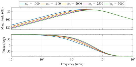
Figure 15. Bode diagram of $H_{\xi -y}\left(s\right)$ by varying the control bandwidth ${\omega }_{ci}$ (${\omega }_{oi}={10}^4$ rad/s).

Figure 16. Bode diagram of $H_{\xi -y}\left(s\right)$ by varying the observer bandwidth ${\omega }_{oi}$ (${\omega }_{ci}=2000$ rad/s).

It should be noted that the practical selection of the observer bandwidth represents a trade-off between estimation speed and noise sensitivity, whereas the controller bandwidth is determined by the required settling time.

4.3. Sliding Mode Control Based on LESO

The nonlinear and variable-structure nature of power converters renders linear feedback control ineffective under strong disturbances that cause significant deviation from the nominal operating point. A suitable controller that deals with these strong disturbances is the well-known Sliding Mode Control (SMC) technique [55]. SMC is prized for its robustness, high accuracy, fast dynamic response, stability, and simple design. These attributes have led to its widespread adoption in applications like robotics, electrical machine control, and power electronics [56,57,58].

Although SMC is an efficient method for eliminating disturbances, it suffers from the major drawback of chattering. The integration of LESO into SMC not only enables accurate estimation of state variables and total disturbances but also mitigates the chattering problem. Sliding mode control based on the linear extended state observer (SMC-LESO) is an advanced strategy that merges the robustness of SMC with the estimation capabilities of LESO [28,48,54,59].

Design of Control Law

The controller design consists of two stages. First, a sliding surface is selected to define the desired asymptotic dynamics. Second, a control law is designed to drive the system’s trajectories toward and maintain them on that surface.

To design the control law, let us consider the augmented state representation (43). For switched converters, it is convenient to have a control law that adopts a switching function defined as

$$\begin{array}{c}\hfill u_i=\left\{\begin{array}{c}{u}_i^{+}\mathrm{when}{\sigma }_i>0\\ u_i^{-}\mathrm{when}{\sigma }_i<0\end{array}\right.\end{array}$$

(56)

where $\sigma$ is a sliding surface given by (57) in such a way that zero tracking error is guaranteed;

$$\begin{array}{cc}\hfill & {\sigma }_i={\alpha }_{1i}{e}_i+{\alpha }_{2i}\int e_i,\forall i\in \{2,3\}\hfill \end{array}$$

(57)

where $e_i=V_{i,\mathrm{ref}}-x_1$ is the sate error and ${\alpha }_{1i}$ and ${\alpha }_{2i}$ are positive sliding coefficients.

To guarantee the stability on the sliding surface, the existence condition of the sliding mode (58) must be satisfied:

$$\begin{array}{cc}\hfill & \underset{{\sigma }_i\to 0}{lim}{\sigma }_i{\dot{\sigma }}_i<0\hfill \end{array}$$

(58)

To make ${\sigma }_i$ attractive, the reaching law is chosen as

$$\begin{array}{cc}\hfill & {\dot{\sigma }}_i=-{\beta }_{1i}{\sigma }_i-{\beta }_{2i}sign\left({\sigma }_i\right),{\beta }_{1i}>0,{\beta }_{2i}>0\hfill \end{array}$$

(59)

Deriving (57) and equating it with (59), the control law is defined as

$$\begin{array}{cc}\hfill & u_i=-{\displaystyle \frac{1}{b_{0,i}}}({\xi }_i-{\displaystyle \frac{{\alpha }_{2i}}{{\alpha }_{1i}}}e-{\beta }_{1i}{\sigma }_i-{\beta }_{2i}sign\left({\sigma }_i\right))\hfill \end{array}$$

(60)

To perform stability analysis, the $Lyapunov$ function is defined as

$$\begin{array}{cc}\hfill & V_i={\displaystyle \frac{1}{2}}{\sigma }_i^2\hfill \end{array}$$

(61)

and its derivative with respect to time is as follows:

$$\begin{array}{cc}\hfill & {\dot{V}}_i={\sigma }_i{\dot{\sigma }}_i\hfill \end{array}$$

(62)

Evaluating $\dot{\sigma }$ and substituting (60), (62) becomes

$$\begin{array}{cc}\hfill & {\dot{V}}_i=-{\alpha }_{1i}|{\sigma }_i|({\beta }_{1i}|{\sigma }_i|+{\beta }_{2i})\hfill \end{array}$$

(63)

Being that ${\alpha }_{1i}$, ${\beta }_{1i}$ and ${\beta }_{2i}$ are positive scalars, ${\dot{V}}_i$ is negative and therefore the asymptotic stability of the system is guaranteed.

It is worth noting that the control law derived so far (Equation (60)) corresponds to conventional SMC. The SMC-based LESO (SMC-LESO) control law is then designed by combining (60) and (45), resulting in the following control law:

$$\begin{array}{cc}\hfill & u_i=-{\displaystyle \frac{1}{b_{0,i}}}({\widehat{\xi }}_i-{\displaystyle \frac{{\alpha }_{2i}}{{\alpha }_{1i}}}{\widehat{e}}_i-{\beta }_{1i}{\widehat{\sigma }}_i-{\beta }_{2i}sign\left({\widehat{\sigma }}_i\right))\hfill \end{array}$$

(64)

where ${\widehat{e}}_i=V_{i,\mathrm{ref}}-z_1$, ${\widehat{\sigma }}_i={\alpha }_{1i}{\widehat{e}}_i+{\alpha }_{2i}\int {\widehat{e}}_i$, and ${\widehat{\xi }}_i=z_2$ are the estimation error, sliding surface, and disturbance, respectively. The block diagram of the SMC-based LESO for TAB converter is depicted in Figure 17.

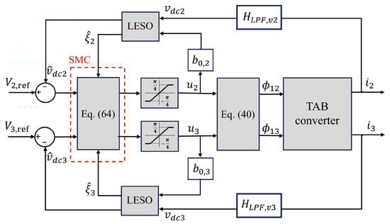
Figure 17. SMC-based LESO block diagram of TAB converter.

It is worth noting that the sliding coefficients ${\alpha }_{ij}$ and ${\beta }_{ij}$ were tuned empirically to balance the fundamental trade-off between response speed, robustness, and chattering mitigation.

4.4. Control Comparison

The performance of the control strategies previously presented is tested based on the circuit depicted in Figure 1. The converter circuit was created in Simulink using the parameters presented in Table 2, which are taken from [17] and slightly modified to assess the control strategies when the TAB operates at different voltage levels. This highlights the ability of the TAB converter to connect sources and loads at different voltage levels, which is an advantage of isolated topologies.

Table 2. TAB converter and control parameters.

	Parameter	Value
TAB Converter	Rated power: $P_1$, $P_2$, $P_3$	$3.5$, 2, $1.5$ kW
	Port voltage: $v_{dc1}$, $v_{dc2}$, $v_{dc3}$	400, 400, 350 V
	Port inductance: $L_1$, $L_2$, $L_3$	$36.7$, $36.5$, $36.8$ µH
	Port resistance: $R_{s1}$, $R_{s2}$, $R_{s3}$	135, 136, 139 m$\Omega$
	Port capacitance: $C_2$, $C_3$	$0.4$, $0.4$ mF
	Switching frequency: $f_s$	20 kHz
IDM	$k_{p2}$, $k_{i2}$	0.0125, 3.125
	$k_{p3}$, $k_{i3}$	0.0122, 3
LADRC	${\omega }_{o2}$, ${\omega }_{c2}$	${10}^4$, 2000 rad/s
	${\omega }_{o3}$, ${\omega }_{c3}$	${10}^4$, 2000 rad/s
SMC-LESO	${\alpha }_{12}$, ${\alpha }_{22}$, ${\beta }_{12}$, ${\beta }_{22}$, ${\omega }_{o2}$	1, ${10}^4$, 1, ${10}^{-3}$, ${10}^4$ (rad/s)
	${\alpha }_{13}$, ${\alpha }_{23}$, ${\beta }_{13}$, ${\beta }_{23}$, ${\omega }_{o3}$	1, ${10}^4$, 1, ${10}^{-3}$, ${10}^4$ (rad/s)

The proposed control strategies are tested considering three consecutive disturbances inducing a transient.

• Load at Port 2 increases from 2 kW to 3 kW at time t = 0.1 s.
• Load at Port 3 increases from 1.5 kW to 3 kW at time t = 0.2 s.
• The input voltage at Port 1 increases from 400 V to 440 V at t = 0.3 s.

These events are selected so that the control strategy is tested when disturbances occur at both output ports. The magnitude of the change is considered large enough for the load, given that a sudden increase could occur in cases such as EV charging connections in household applications or microgrid interconnection reconfiguration, leading to power flow changes. On the other hand, sudden voltage changes are not expected to happen, so a 10% disturbance is considered for the input voltage. The output voltage responses in Port 2 and Port 3 are shown in Figure 18, Figure 19 and Figure 20. The figures present a comparative analysis of the decoupling performance of three control strategies applied to a TAB converter.

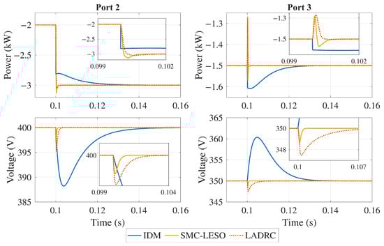
Figure 18. Output power ($P_2,P_3$) and voltage ($v_{d{c}_2},v_{d{c}_3}$) response under load disturbances in Port 2.

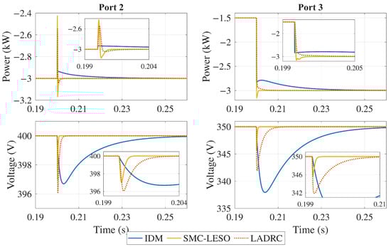
Figure 19. Output power ($P_2,P_3$) and voltage ($v_{d{c}_2},v_{d{c}_3}$) response under load disturbances in Port 3.

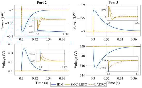
Figure 20. Output power ($P_2,P_3$) and voltage ($v_{d{c}_2},v_{d{c}_3}$) response under input voltage disturbances.

As can be seen, the controllers exhibit distinct performance characteristics. The IDM controller experiences a significant overshoot due to cross-coupling effects. In contrast, the LADRC controller performs better, exhibiting a smaller voltage dip and faster settling time. However, the SMC-LESO outperforms both by maintaining the voltage closer to its nominal value with minimal deviation and rapid recovery, showcasing its strong robustness and effective decoupling capabilities.

The robustness of the decoupling control strategies is also assessed under parameter uncertainties in the TAB converter. Figure 21 shows the voltage response at Ports 2 and 3 under a severe deviation in Port 2 leakage inductance ($L_2^{new}=2L_2$). The results indicate a certain degree of robustness in all three controllers. Both the LADRC and SMC-LESO controllers exhibit stronger robustness against parameter uncertainties, maintaining minimal voltage deviation and small settling time with effective disturbance rejection. In contrast, the IDM controller experiences a significant voltage drop and a larger settling time. Moreover, the voltage derivation is much larger than when $L_2$ was considered as a well-known parameter (see Figure 20), revealing a high sensitivity to inaccuracies in the converter’s parameters.

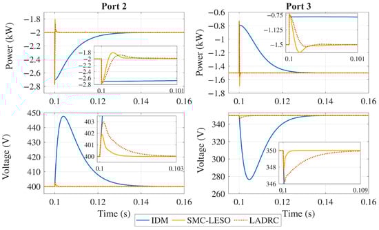
Figure 21. Output power ($P_2,P_3$) and voltage ($v_{d{c}_2},v_{d{c}_3}$) response under load disturbance in Port 2 and with deviations in the value of Port 2 leakage inductance $L_2$.

Among the three methods, IDM imposes the highest computational load due to its reliance on real-time matrix inversion, which scales poorly and is highly sensitive to model errors. On the other hand, LADRC is more efficient, leveraging a simple LESO, but its performance is constrained in practice by sensor noise and the choice of $b_{0i}$. Additionally, SMC-LESO implementation is challenged by control chattering, forcing a trade-off between robustness and smoothness that complicates tuning. Thus, for real-time systems, LADRC typically offers a better balance of efficiency and performance. SMC-LESO provides superior disturbance rejection at the cost of greater tuning effort, and inverse decoupling is the least suitable for resource-constrained applications.

5. Conclusions

This paper presented the TAB converter operation, modeling, and control approaches. The operation was briefly summarized, introducing the reader to different operation modes and modulation methods. The generalized average model and the ROMs’ large-signal representation were compared under different operating conditions. Both models correctly represent the dynamic and power flow behavior of the converter. However, the first harmonic approximation used in the generalized average model limits the power flow representation, which is reflected in the voltage level achieved when the phase shift values of each port are fixed. On the other hand, the ROM represents the power flow dynamics better when the phase shift at both output ports is equal, leaving little to no port coupling. However, under highly coupled operating conditions, the advantages of the ROM are not as obvious. Therefore, the models should be carefully used, depending on the operating point.

The control strategies studied in this work aim to improve the dynamic response of the TAB by decoupling or mitigating the magnetically coupled nature of the TAB converter output ports’ dynamics. The interdependent power flows between its ports make the controller design a major challenge. To address this, three strategies were derived based on a ROM: IDM, LADRC, and SMC-LESO. Their performance was evaluated under external disturbances and parametric uncertainties. A comprehensive comparison between these control strategies clearly shows that SMC-LESO provides the best decoupling performance, maintaining voltage regulation across all ports and faster stabilization. LADRC also offers significant improvement over the IDM strategy. Despite their conceptual simplicity and the fact that IDM strategy decomposes the TAB converter into independent SISO systems, their practical application is constrained by high sensitivity to operating point variations and model uncertainties. In contrast, LADRC, and SMC-LESO overcome these limitations through robust disturbance rejection, inherent insensitivity to model inaccuracies, and the real-time estimation and compensation of coupling effects by a LESO, thereby enhancing system robustness and reliability. However, the LESO design remains critical, as inadequate implementation compromises state variable tracking and ultimately degrades control performance. A well-designed LESO is key to enabling LADRC and SMC-LESO as robust solutions for decoupling power flows in the TAB converter.

Future work will be focused on an improved generalized average model that better represents the TAB converter, leaving the computation burden unaffected. Furthermore, the use of the TAB in power grid solutions, such as the soft open points and solid state transformer, will be studied. Additionally, an experimental setup is under development and will be used in experimental validation of the control strategies presented in this study.

References

- Domínguez, R.; Conejo, A.J.; Carrión, M. Toward Fully Renewable Electric Energy Systems. IEEE Trans. Power Syst. 2015, 30, 316–326. [Google Scholar] [CrossRef]
- Zsiborács, H.; Baranyai, N.H.; Vincze, A.; Zentkó, L.; Birkner, Z.; Máté, K.; Pintér, G. Intermittent Renewable Energy Sources: The Role of Energy Storage in the European Power System of 2040. Electronics 2019, 8, 729. [Google Scholar] [CrossRef]
- Zhao, B.; Song, Q.; Liu, W.; Sun, Y. Overview of Dual-Active-Bridge Isolated Bidirectional DC–DC Converter for High-Frequency-Link Power-Conversion System. IEEE Trans. Power Electron. 2014, 29, 4091–4106. [Google Scholar] [CrossRef]
- Costa, P.F.S.; Löbler, P.H.B.; Roggia, L.; Schuch, L. Modeling and Control of DAB Converter Applied to Batteries Charging. IEEE Trans. Energy Convers. 2022, 37, 175–184. [Google Scholar] [CrossRef]
- Harrison, S.; Soltoswski, B.; Pepiciello, A.; Henao, A.C.; Farag, A.Y.; Beza, M.; Xu, L.; Egea-Àlvarez, A.; Cheah-Mañé, M.; Gomis-Bellmunt, O. Review of multiport power converters for distribution network applications. Renew. Sustain. Energy Rev. 2024, 203, 114742. [Google Scholar] [CrossRef]
- Pereira, T.; Hoffmann, F.; Zhu, R.; Liserre, M. A Comprehensive Assessment of Multiwinding Transformer-Based DC–DC Converters. IEEE Trans. Power Electron. 2021, 36, 10020–10036. [Google Scholar] [CrossRef]
- Byun, H.J.; Kim, S.H.; Lee, Y.S.; Yi, J.; Won, C.Y. Control Strategy of Triple-Active-Bridge Converter for Bipolar DC Microgrid. IEEE Trans. Ind. Electron. 2024, 71, 10658–10668. [Google Scholar] [CrossRef]
- Wu, Y.; Mahmud, M.H.; Christian, S.; Fantino, R.A.; Gomez, R.A.; Zhao, Y.; Balda, J.C. A 150-kW 99Converter for Solar-Plus-Storage Systems. IEEE J. Emerg. Sel. Top. Power Electron. 2022, 10, 3496–3510. [Google Scholar] [CrossRef]
- Hoffmann, F.; Person, J.; Andresen, M.; Liserre, M.; Freijedo, F.D.; Wijekoon, T. A Multiport Partial Power Processing Converter With Energy Storage Integration for EV Stationary Charging. IEEE J. Emerg. Sel. Top. Power Electron. 2022, 10, 7950–7962. [Google Scholar] [CrossRef]
- Chandwani, A.; Mallik, A. Phase-Duty Modulated Loop Decoupling and Design Optimization for a Triple Active Bridge Converter for Light Electric Vehicle Charging. IEEE J. Emerg. Sel. Top. Ind. Electron. 2023, 4, 357–367. [Google Scholar] [CrossRef]
- Cao, H.; Du, L.; Guo, F.; Ma, Z.; Zhao, Y. A Triple Active Bridge (TAB) Based Solid-State Transformer (SST) for DC Fast Charging Systems: Architecture and Control Strategy. In Proceedings of the 2023 IEEE Energy Conversion Congress and Exposition (ECCE), Nashville, TN, USA, 29 October–2 November 2023; pp. 855–860. [Google Scholar] [CrossRef]
- Gabriel, M.T.; Mansour, D.E.A.; Shoyama, M.; Abdelkader, S.M. A Triple-Active Bridge Based Solid State Transformer Fast Charging Station Topology For Electric Vehicles. In Proceedings of the 2024 IEEE International Conference on Environment and Electrical Engineering and 2024 IEEE Industrial and Commercial Power Systems Europe (EEEIC/I&CPS Europe), Rome, Italy, 17–20 June 2024; pp. 01–06. [Google Scholar] [CrossRef]
- Uttam, V.; Iyer, V.M. A Unified Modeling Approach for Steady State and ZVS Analysis of a Triple Active Bridge Converter. IEEE Trans. Ind. Appl. 2024, 60, 8950–8962. [Google Scholar] [CrossRef]
- Purgat, P.; Bandyopadhyay, S.; Qin, Z.; Bauer, P. Zero Voltage Switching Criteria of Triple Active Bridge Converter. IEEE Trans. Power Electron. 2021, 36, 5425–5439. [Google Scholar] [CrossRef]
- Yang, J.; Buticchi, G.; Gu, C.; Günter, S.; Zhang, H.; Wheeler, P. A Generalized Input Impedance Model of Multiple Active Bridge Converter. IEEE Trans. Transp. Electrif. 2020, 6, 1695–1706. [Google Scholar] [CrossRef]
- Sanders, S.R.; Noworolski, J.M.; Liu, X.Z.; Verghese, G.C. Generalized Averaging Method for Power Conversion Circuits. IEEE Trans. Power Electron. 1991, 6, 251–259. [Google Scholar] [CrossRef]
- Okutani, S.; Huang, P.Y.; Kado, Y. Generalized average model of triple active bridge converter. In Proceedings of the 2019 IEEE Energy Conversion Congress and Exposition (ECCE), Baltimore, MD, USA, 29 September–3 October 2019. [Google Scholar]
- Purgat, P.; Bandyopadhyay, S.; Qin, Z.; Bauer, P. Continuous Full Order Model of Triple Active Bridge Converter. In Proceedings of the 2019 21st European Conference on Power Electronics and Applications (EPE ’19 ECCE Europe), Genova, Italy, 3–5 September 2019; pp. P.1–P.9. [Google Scholar] [CrossRef]
- Henao-Muñoz, A.C.; Pepiciello, A.; Debbat, M.; Tarrasó, A.; Domínguez-García, J.L. State Space Modeling and Small-Signal Stability Analysis of a Multiport Soft Open Point Based on the Triple Active Bridge Converter. In Proceedings of the 2024 International Conference on Smart Energy Systems and Technologies (SEST), Torino, Italy, 10–12 September 2024; pp. 1–6. [Google Scholar] [CrossRef]
- Bandyopadhyay, S.; Purgat, P.; Qin, Z.; Bauer, P. A Multiactive Bridge Converter With Inherently Decoupled Power Flows. IEEE Trans. Power Electron. 2021, 36, 2231–2245. [Google Scholar] [CrossRef]
- Koohi, P.; Watson, A.J.; Clare, J.C.; Soeiro, T.B.; Wheeler, P.W. A Survey on Multi-Active Bridge DC-DC Converters: Power Flow Decoupling Techniques, Applications, and Challenges. Energies 2023, 16, 5927. [Google Scholar] [CrossRef]
- Henao-Muñoz, A.C.; Pepiciello, A.; Domínguez-García, J.L. Control Strategy for a Triple Active Bridge Converter: A Generalized Average Model Approach. In Proceedings of the 2023 IEEE PES Innovative Smart Grid Technologies Europe (ISGT EUROPE), Grenoble, France, 23–26 October 2023; pp. 1–5. [Google Scholar] [CrossRef]
- Purgat, P.; Bandyopadhyay, S.; Qin, Z.; Bauer, P. Power Flow Decoupling Controller for Triple Active Bridge Based on Fourier Decomposition of Transformer Currents. In Proceedings of the 2020 IEEE Applied Power Electronics Conference and Exposition (APEC), New Orleans, LA, USA, 15–19 March 2020; pp. 1201–1208. [Google Scholar] [CrossRef]
- Zhao, C.; Round, S.D.; Kolar, J.W. An Isolated Three-Port Bidirectional DC-DC Converter With Decoupled Power Flow Management. IEEE Trans. Power Electron. 2008, 23, 2443–2453. [Google Scholar] [CrossRef]
- Koya, N.; Yuichi, K.; Keiji, W. Implementation of Decoupling Power Flow Control System in Triple Active Bridge Converter Rated at 400V, 10kW, and 20kHz. IEEJ J. Ind. Appl. 2018, 7, 410–415. [Google Scholar] [CrossRef]
- Debbat, M.B.; Henao-Muñoz, A.C.; Pepiciello, A.; Domínguez-García, J.L. Sliding-Mode Based Control Technique for Triple Active Bridge DC-DC Converter. In Proceedings of the 2024 XV International Symposium on Industrial Electronics and Applications (INDEL), Banja Luka, Bosnia and Herzegovina, 6–8 November 2024; pp. 1–6. [Google Scholar] [CrossRef]
- Bandyopadhyay, S.; Qin, Z.; Bauer, P. Decoupling Control of Multiactive Bridge Converters Using Linear Active Disturbance Rejection. IEEE Trans. Ind. Electron. 2021, 68, 10688–10698. [Google Scholar] [CrossRef]
- Gong, S.; Li, X.; Han, J.; Sun, Y.; Xu, G.; Jiang, Y.; Huang, S. Sliding Mode Control-Based Decoupling Scheme for Quad-Active Bridge DC–DC Converter. IEEE J. Emerg. Sel. Top. Power Electron. 2022, 10, 1153–1164. [Google Scholar] [CrossRef]
- Adam, A.H.A.; Chen, J.; Kamel, S.; Ahmed, E.M.; Zaki, Z.A. Improved dynamic performance of triple active bridge DC-DC converter using differential flatness control for more electric aircraft applications. Results Eng. 2024, 23, 102811. [Google Scholar] [CrossRef]
- Buticchi, G.; Farjudian, A.; Oh, J.; Tarisciotti, L. An ANN-Assisted Control for the Power Decoupling of a Multiple Active Bridge DC-DC Converter. In Proceedings of the IECON 2022—48th Annual Conference of the IEEE Industrial Electronics Society, Brussels, Belgium, 17–20 October 2022. [Google Scholar]
- Liao, M.; Li, H.; Wang, P.; Sen, T.; Chen, Y.; Chen, M. Machine Learning Methods for Feedforward Power Flow Control of Multi-Active-Bridge Converters. IEEE Trans. Power Electron. 2023, 38, 1692–1707. [Google Scholar] [CrossRef]
- Qiu, R.; Gu, C.; Li, J.; Yang, J. A Simplified ANN Based Power Decoupling Method of MAB Converters. In Proceedings of the 2025 IEEE 8th International Electrical and Energy Conference (CIEEC), Changsha, China, 16–18 May 2025. [Google Scholar]
- Mukherjee, S.; Sarkar, I. A Brief Review on Triple Active Bridge DC-DC Converter. In Proceedings of the 2023 IEEE International Students’ Conference on Electrical, Electronics and Computer Science (SCEECS), Bhopal, India, 18–19 February 2023; pp. 1–6. [Google Scholar] [CrossRef]
- Shao, S.; Chen, L.; Shan, Z.; Gao, F.; Chen, H.; Sha, D.; Dragičević, T. Modeling and Advanced Control of Dual-Active-Bridge DC–DC Converters: A Review. IEEE Trans. Power Electron. 2022, 37, 1524–1547. [Google Scholar] [CrossRef]
- He, J.; Chen, Y.; Lin, J.; Chen, J.; Cheng, L.; Wang, Y. Review of Modeling, Modulation, and Control Strategies for the Dual-Active-Bridge DC/DC Converter. Energies 2023, 16, 6646. [Google Scholar] [CrossRef]
- Tarraf, R.; Frey, D.; Leirens, S.; Carcouet, S.; Maynard, X.; Lembeye, Y. Modeling and Control of a Hybrid-Fed Triple-Active Bridge Converter. Energies 2023, 16, 6007. [Google Scholar] [CrossRef]
- De Doncker, R.W.; Divan, D.M.; Kheraluwala, M.H. A Three-Phase Soft-Switched High-Power-Density DC-DC Converter for High-Power Applications. IEEE Trans. Ind. Appl. 1991, 27, 63–73. [Google Scholar] [CrossRef]
- Duarte, J.L.; Hendrix, M.; Simoes, M.G. Three-Port Bidirectional Converter for Hybrid Fuel Cell Systems. IEEE Trans. Power Electron. 2007, 22, 480–487. [Google Scholar] [CrossRef]
- Gong, L.; Xu, J.; Zhao, J.; Li, W.; Wang, T.; Peng, Y.; Wang, Y.; Soeiro, T.B. A Simplified All-ZVS Strategy for High-Frequency Triple Active Bridge Converters With Designed Magnetizing Inductance. IEEE Trans. Power Electron. 2023, 38, 13781–13797. [Google Scholar] [CrossRef]
- Bacha, S.; Munteanu, I.; Bratcu, A.I. Power Electronic Converters Modeling and Control: With Case Studies; Advanced Textbooks in Control and Signal Processing; Springer: London, UK, 2014. [Google Scholar] [CrossRef]
- Rodríguez Alonso, A.R.; Sebastian, J.; Lamar, D.G.; Hernando, M.M.; Vazquez, A. An overall study of a Dual Active Bridge for bidirectional DC/DC conversion. In Proceedings of the 2010 IEEE Energy Conversion Congress and Exposition, Atlanta, GA, USA, 12–16 September 2010; pp. 1129–1135. [Google Scholar] [CrossRef]
- Kundur, P. Power System Stability and Control; McGraw-Hill: New York, NY, USA, 2007. [Google Scholar]
- Shah, S.S.; Bhattacharya, S. Large & small signal modeling of dual active bridge converter using improved first harmonic approximation. In Proceedings of the 2017 IEEE Applied Power Electronics Conference and Exposition (APEC), Tampa, FL, USA, 26–30 March 2017; pp. 1175–1182. [Google Scholar] [CrossRef]
- Biswas, I.; Kastha, D.; Bajpai, P. Small signal modeling and decoupled controller design for a triple active bridge multiport DC-DC converter. IEEE Trans. Power Electron. 2020, 36, 1856–1869. [Google Scholar] [CrossRef]
- Han, J. Extended state observer for a class of uncertain plants. Chin. Control Decis. 1995, 10, 85–88. [Google Scholar]
- Gao, Z. Active disturbance rejection control: A paradigm shift in feedback control system design. In Proceedings of the 2006 American Control Conference, Minneapolis, MN, USA, 14–16 June 2006. [Google Scholar]
- Han, J. From PID to active disturbance rejection control. IEEE Trans. Ind. Electron. 2009, 56, 900–906. [Google Scholar] [CrossRef]
- Wang, J.; Li, S.; Yang, J.; Wu, B.; Li, Q. Extended state observer-based sliding mode control for PWM-based DC–DC buck power converter systems with mismatched disturbances. IET Control Theory Appl. 2015, 9, 579–586. [Google Scholar] [CrossRef]
- Yang, J.; Cui, H.; Li, S.; Zolotas, A. Optimized active disturbance rejection control for DC–DC buck converters with uncertainties using a reduced-order GPI observer. IEEE Trans. Circuits Syst. I Regul. Pap. 2018, 65, 832–841. [Google Scholar] [CrossRef]
- Ahmad, S.; Ali, A. Active disturbance rejection control of DC–DC boost converter: A review with modifications for improved performance. IET Power Electron. 2019, 12, 2095–2107. [Google Scholar] [CrossRef]
- Zhuo, S.; Gaillard, A.; Xu, L.; Paire, D.; Gao, F. Extended state observer-based control of DC–DC converters for fuel cell application. IEEE Trans. Power Electron. 2020, 35, 9923–9932. [Google Scholar] [CrossRef]
- Hua, X. Full-bridge DC-DC Converter based on Linear Active Disturbance Rejection Control. Front. Comput. Intell. Syst. 2025, 11, 2832–6024. [Google Scholar] [CrossRef]
- Gao, Z. Scaling and bandwidth-parameterization based controller tuning. In Proceedings of the 2003 American Control Conference, Denver, CO, USA, 4–6 June 2003. [Google Scholar]
- Yang, M.; Liu, P. Research on Sliding Mode Control of Dual Active Bridge Converter Based on Linear Extended State Observer in Distributed Electric Propulsion System. Electronics 2023, 12, 3522. [Google Scholar] [CrossRef]
- Utkin, V.I. Sliding mode control design principles and applications to electric drives. IEEE Trans. Ind. Electron. 1993, 40, 6783–6800. [Google Scholar] [CrossRef]
- Sira-Ramirez, H. Sliding Motions in Bilinear Switched Network. IEEE Trans. Cir. Sys. 1987, 35, 919–933. [Google Scholar]
- Mattavelli, P.; Rossetto, L.; Spiazzi, G. Small-signal analysis of DC–DC converters with sliding mode control. IEEE Trans. Power Electron. 1997, 12, 69–102. [Google Scholar] [CrossRef]
- Martınez-Salamero, L.; Calvente, J.; Giral, R.; Poveda, A.; Fossas, E. Analysis of a bidirectional coupled-inductor Cuk converter operating in sliding mode. IEEE Trans. Circit Syst. 1998, 45, 355–363. [Google Scholar] [CrossRef]
- Ma, F.; Yang, Z.; Ji, P. Sliding Mode Controller Based on the Extended State Observer for Plant-Protection Quadrotor Unmanned Aerial Vehicles. Mathematics 2022, 10, 1346. [Google Scholar] [CrossRef]
Disclaimer/Publisher’s Note: The statements, opinions and data contained in all publications are solely those of the individual author(s) and contributor(s) and not of MDPI and/or the editor(s). MDPI and/or the editor(s) disclaim responsibility for any injury to people or property resulting from any ideas, methods, instructions or products referred to in the content. |
© 2025 by the authors. Licensee MDPI, Basel, Switzerland. This article is an open access article distributed under the terms and conditions of the Creative Commons Attribution (CC BY) license (https://creativecommons.org/licenses/by/4.0/).