Equivalent Modeling Method for Thermal Calculation of Transformer Windings Based on Minimum Thermal Resistance

Abstract

In the accurate calculation of the temperature rise and hot spots of transformer windings, considering the inter-turn insulation will lead to a sharp increase in the workload of detailed modeling and a large number of mesh refinements. To address this issue, this paper proposes a calculation method for the equivalent thermal conductivity based on the minimum thermal resistance principle. This method can accurately calculate the equivalent thermal conductivities in the axial and radial directions of the windings. By using the disk windings model under the equivalent thermal conductivity, a temperature field analysis is performed on the actual windings with inter-turn insulation. To validate the method, models considering inter-turn insulation and equivalent models are constructed, and detailed analyses are performed using the empirical formula method and the equivalent method based on the minimum thermal resistance principle, respectively. By comparing the simulation results of the equivalent model and the model considering inter-turn insulation, it is found that the equivalent method based on the minimum thermal resistance principle not only significantly reduces the number of mesh elements but also achieves significantly improved accuracy in the temperature field analysis of the turn-divided model compared to the empirical formula method. Moreover, the winding temperature rise and hot spot positions before and after the equivalence are nearly identical and closer to the experimental results, demonstrating the validity of this method.

1. Introduction

The power transformer is one of the most important components in the power system, and its safe and stable operation for a long time is crucial [1,2]. However, transformer life is directly related to the winding temperature, and most transformer failures are caused by high winding temperatures [3,4]. Therefore, fast and accurate prediction of transformer winding temperature is of great significance to prolong the transformer life and ensure the stable operation of the power system, which has received a lot of attention from scholars.

The existing predominant approaches for predicting power transformer temperatures include the numerical analysis method, the empirical formula method, and the lumped parameter method.

The hot-spot temperature of the power transformer windings can be obtained by direct measurement [4,5]. That is, the fiber optic probe or thermocouple is placed in the hot spot area for measurement, but this method requires the placement of a temperature sensor before the transformer is put into operation, and it is not applicable to the transformer that has been put into operation. In addition, there are hot path model methods, empirical formula methods, artificial intelligence algorithms, and multiphysics modeling calculation methods to determine hot spot temperatures [6,7,8,9].

Thermal conductivity refers to a material’s ability to conduct heat and is a fundamental thermal property, particularly critical in solid-state heat transfer applications. Accurate determination of thermal conductivity is essential for the design and evaluation of materials used in electronics, insulation, energy systems, and many other engineering fields. There are numerous experimental techniques available to measure thermal conductivity; however, they can broadly be classified into two main categories: steady-state methods and transient (or non-steady-state) methods [10]. However, no method can be applied to all application fields, measurement ranges, accuracies, or sample shapes and sizes [11,12]. With the rapid development of composite materials, the research and testing of thermal conductivity have expanded beyond single-phase materials. Reference [13] used the model matrix to accurately calculate the thermal conductivity of the material and optimized the calculation model to ensure accuracy. Reference [14] describes the influence of single-layer and multi-layer metal graphene composite materials on thermal conductivity and discusses the overall thermal conductivity based on the anisotropy of the materials. In this context, effective thermal conductivity (ETC) has emerged as a critical parameter for evaluating the overall heat conduction performance of composites, which often consist of multiple heterogeneous phases. The measurement, prediction, and optimization of ETC have thus become key research focuses in the field of composite materials. These efforts aim to understand the complex heat transfer mechanisms within multiphase systems and to design materials with tailored thermal properties for advanced engineering applications such as thermal management, energy storage, and electronics cooling [15,16].

Reference [17] took into account the influence of solar radiation on the hot-spot temperature of transformers. Meanwhile, it provided nonlinear parameters for the thermal circuit model in terms of oil flow density, thermal conductivity, specific heat capacity, and dynamic viscosity, which affect the calculation accuracy of the thermal circuit model, and thus improved the calculation model of the transformer hot-spot temperature. The average fluid velocity was obtained through a 3D flow field simulation, and the overall temperature rise in the transformer was calculated using a thermal network model. Comparison with experimental and numerical results showed that the method had controllable error and high computational efficiency, providing a reliable basis for transformer thermal analysis and temperature rise prediction [18,19]. The fluid–thermal network model (THNM) was extended to encompass the entire transformer room. By accounting for air thermal buoyancy and pressure losses in airflow, a detailed flow path within the transformer room was constructed. A comprehensive thermal network model, incorporating walls and roofs, was developed to simulate the thermal behavior of the space. This extension enabled more accurate temperature analysis within the transformer room, thereby further enhancing the overall precision of the THNM [20].

In current simulations of transformer winding temperature rise and hot spot distribution, windings composed of multiple split turns are often simplified into equivalent winding disks to reduce modeling complexity. However, this simplification typically neglects the thermal resistance introduced by inter-turn insulation, resulting in significant discrepancies between simulated and actual temperature rise and hot spot predictions.

To address this issue and strike a balance between modeling accuracy and computational efficiency, this paper proposes an equivalent thermal circuit model of the windings based on the principle of minimum thermal resistance. This approach enables the determination of equivalent thermal conductivities in both axial and radial directions of the winding structure.

A two-dimensional model of oil-immersed power transformer windings is taken as the case study. The windings are equivalently modeled using both an empirical formula method and the proposed minimum thermal resistance method. Comparative analysis with experimental results demonstrates that the proposed method significantly improves the accuracy of temperature rise predictions, thereby validating its effectiveness for engineering applications in transformer thermal design and evaluation.

2. Equivalent Thermal Conductivity Calculation Method

2.1. Equivalent Thermal Conductivity Calculation Method Based on the Law of Minimum Thermal Resistance

Drawing an analogy between the heat transfer process and the conduction of an electric current in a circuit, the thermal resistance is similar to a resistor, the temperature difference is similar to voltage, and the heat flow is similar to an electric current. According to Ohm’s law, the current will give preference to the path with the least resistance, and in the same way, during heat transfer, the heat flow will also give preference to the path with the least thermal resistance to transfer heat:

$$\mathrm{\Delta }{T}_r=R·q$$

(1)

where ΔΤr is the thermal resistance, R is the thermal resistance, and q is the heat conducted per unit time, also known as the thermal conductivity rate. For the parallel hot path channels, the thermal resistance is the same, and the heat flow is the maximum, and the thermal resistance is the minimum, which is the equivalent thermal resistance value. For homogeneous media:

$$R=L/(A\cdot \lambda )$$

(2)

where L is the length of the thermal resistance channel and A is the thermal conductivity area; λ is the thermal conductivity. For composites such as oil-immersed power transformer windings, there is a formula

$$R_{\mathrm{e}}=L/(A\cdot {\lambda }_{\mathrm{e}})$$

(3)

Borrowing the principles and methods of circuits, the thermal resistance is compared to resistance, and the equivalent thermal resistance is obtained by applying the principle of series and parallel connection of circuits. At the same time, to simplify the calculation, materials with the same thermal conductivity in the same heat flow direction are equivalent to one channel.The schematic diagram is shown in Figure 1.

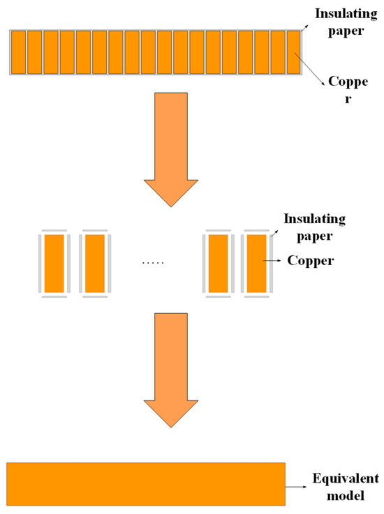
Figure 1. Schematic diagram of coil equivalence.

2.2. Equivalent Thermal Conductivity Calculation Method Based on Analytic Formula

When the heat conduction is stable, because the heat conduction Q does not change with time, that is, the heat conductivity per unit time is a fixed value, the basic equation of heat conductivity can be written as follows:

$$q={\displaystyle \frac{Q}{\tau }}=-\lambda A({\displaystyle \frac{\mathrm{d}T}{\mathrm{d}n}})$$

(4)

where q is the heat conducted per unit time, also known as the thermal conductivity [J/s] or [W]; A is the thermal conductivity area [m²] (is the proportional coefficient, called the thermal conductivity [W/(m·K)]; dT/dn is the temperature gradient [K/m], which indicates the intensity of the temperature change in the direction of heat flow. As shown in Figure 2 and Figure 3. The larger the temperature gradient, the greater the temperature difference per unit length in the direction of heat flow.

$$q={\displaystyle \frac{{\lambda }_{veq}A\mathsf{\Delta }T}{{\delta }_{veq}}}={\displaystyle \frac{A\mathsf{\Delta }T}{\frac{{\delta }_1}{{\lambda }_1}+\frac{{\delta }_2}{{\lambda }_2}+\frac{{\delta }_3}{{\lambda }_3}}}$$

(5)

$${\lambda }_{eq}={\displaystyle \frac{{\delta }_{eq}}{\frac{{\delta }_1}{{\lambda }_1}+\frac{{\delta }_2}{{\lambda }_2}+\frac{{\delta }_3}{{\lambda }_3}}}$$

(6)

where δ_veq is the total thickness of the axial windings disk and λ_veq is the axial equivalent thermal conductivity coefficient of the windings disk.

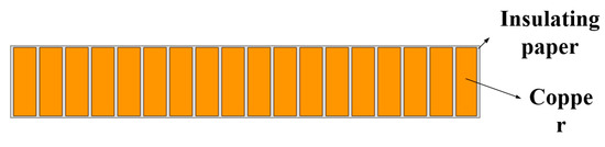
Figure 2. Coil of the split-turn model.

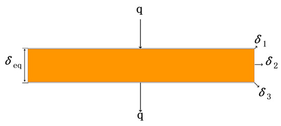
Figure 3. Axial equivalence diagram of the coil.

As shown in Figure 4, the same is true for the radial thermal conductivity, which ignores axial turn insulation and considers only radial turn insulation.

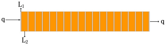
Figure 4. Coil radial equivalence.

L1 is the radial thickness of the insulating paper, L2 is the radial thickness of copper, is the thermal conductivity of the insulating paper diameter, is the thermal conductivity of the copper diameter. Then the radial thermal conductivity is as follows:

$${\lambda }_{eq}={\displaystyle \frac{L_1+L_2}{\frac{L_1}{{\lambda }_1}+\frac{L_2}{{\lambda }_2}}}$$

(7)

3. Simplify the Windings Model

Take a partition windings disk as shown in Figure 5 for equivalent modeling and analysis to ensure that the heat path and boundary conditions before and after the equivalence are the same, and the model with different areas before and after the equivalence needs to change the density of the loss body to ensure that the heat conduction per unit time before and after the equivalence is unchanged.

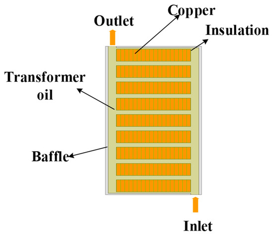
Figure 5. Coil model of equivalent front partition.

To evaluate the accuracy and computational efficiency of the proposed equivalent model, a detailed turn-splitting model incorporating inter-turn insulation was employed as the control group. Under the condition of consistent mesh quality (deviation < 0.8), the turn-splitting model contained 9831 mesh elements. In contrast, the equivalent model—developed using the effective thermal conductivity approach based on the principle of minimum thermal resistance—comprised only 3453 mesh elements. This represents a 65% reduction in mesh count compared to the control model. The finite element calculation time was saved by 80%, significantly improving computational efficiency while maintaining reliable accuracy.

The physical property parameters adopted in the model are detailed in Table 1. In order to reduce modeling complexity while maintaining thermal accuracy, the pre-turn windings structure shown in Figure 5 is equivalently transformed into a simplified windings disk configuration, as illustrated in Figure 6. The equivalent disk is assumed to be made of copper, and its thermal conductivity parameters are defined using equivalent values calculated in both the axial and radial directions.

Table 1. Physical property parameters of materials.

Material	Parameter	Numeric Values and Expressions
Transformer oil	Density/kg·m−3	1098.72 − 0.712T
	Specific heat capacity/J·(kg·K)−1	807.163 + 3.58T
	Thermal conductivity/W·(m·K)−1	0.159 − 7.101 × 10−5T
	Dynamic viscosity/Pa·s	0.8467 − 0.0004T + 5 × 10−7T2
Insulating paper	Density/kg·m−3	980
	Specific heat capacity/J·(kg·K)−1	2000
	Thermal conductivity/W·(m·K)−1	0.25
Copper	Density/kg·m−3	8960
	Specific heat capacity/J·(kg·K)−1	381
	Thermal conductivity/W·(m·K)−1	387.6

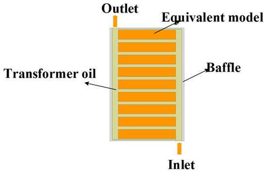
Figure 6. Equivalent post-partition coil model.

Specifically, using the equivalent thermal conductivity method based on the principle of minimum thermal resistance, the axial and radial thermal conductivities are determined to be 2.367 W/(m·K) and 0.4439 W/(m·K), respectively. In contrast, the empirical formula method yields higher equivalent conductivities, with values of 10.295 W/(m·K) in the axial direction and 1.821 W/(m·K) in the radial direction. This comparison highlights the significant difference in estimated thermal parameters between the two methods, which has direct implications for the accuracy of thermal simulations and hot spot prediction in transformer windings.

In the simulation setup, the lower inlet of the model is assigned velocity and temperature boundary conditions, with a vertical inflow velocity of 0.01 m/s and an inlet temperature of 300 K. Different volumetric heat flux densities are applied to the two models: for the equivalent pre-turn model, the loss density is 737,688 W/m³, while for the equivalent windings model, it is 606,680 W/m³.

The outlet is defined as a pressure boundary condition to allow free flow discharge. The surfaces of the windings and baffles are specified as wall boundaries and treated as adiabatic (no heat transfer). Additionally, the winding surfaces are defined as no-slip wall boundary conditions to enable fluid–structure interaction, ensuring accurate thermal–fluid coupling in the simulation.

4. Verification of Simulation Model Accuracy

The temperature field simulation results of each equivalent model are shown in Figure 7, Figure 8 and Figure 9, which are the split-turn model considering inter-turn insulation, the equivalent model based on the minimum thermal resistance rule, and the temperature field simulation results of the model after empirical formula equivalence.

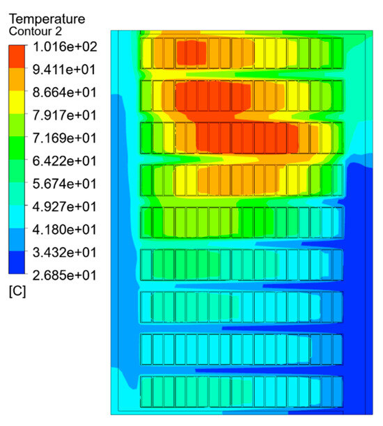
Figure 7. Temperature distribution of the split-turn model.

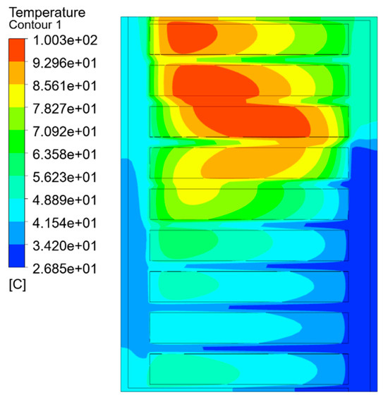
Figure 8. Temperature distribution of the minimum thermal resistance model.

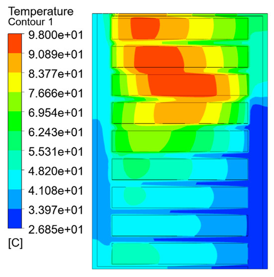
Figure 9. Temperature distribution of the model after the equivalence of the empirical formula.

As can be seen from the temperature field contour and Table 2, the simulation results obtained by the split-turn model and the equivalent model of the minimum thermal resistance method are basically consistent, and the difference is not obvious, with an average temperature error percentage of 0.68% and a temperature error of 2.322 K. The hot-spot error percentage is 1.28%, and the hot-spot temperature error is 1.3 K. The average temperature error percentage of the empirical formula method is 1.15%, and the temperature error is 4.082 K. The percentage of hot-spot error is 3.52%, and the temperature error is 3.6 K. Compared with the empirical formula method, the average temperature and hot-spot temperature errors of the equivalent model of the minimum thermal resistance method are reduced by 60% and 40%, respectively.

Table 2. Temperature and temperature error of each model.

Model	Average Temperature	Hot Spot Temperature	Average Error	Hot Spot Error
Split-turn model	67.484	101.6
Empirical formula	63.402	98.0	1.15%	3.52%
Equivalent model	65.162	100.3	0.68%	1.28%

Figure 10, Figure 11 and Figure 12 show the radial temperature comparison of the pie split-turn model of Line 1, the equivalent model of the empirical formula method, and the equivalent model of the minimum thermal resistance method. The radial temperature of the equivalent model of the minimum thermal resistance method is closer to the distribution of the equivalent model of the empirical formula method than that of the equivalent model of the empirical formula method, and the radial temperature error percentage is 0.25% and 2.5% at the minimum. The radial temperature error is 0.25 °C at least and 2.2 °C at the maximum.

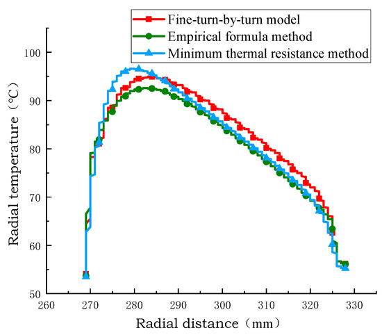
Figure 10. Comparison of radial temperature of coil no.1.

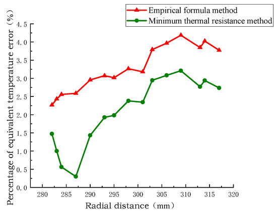
Figure 11. Comparison of the percentage of radial temperature error of windings disk no.1.

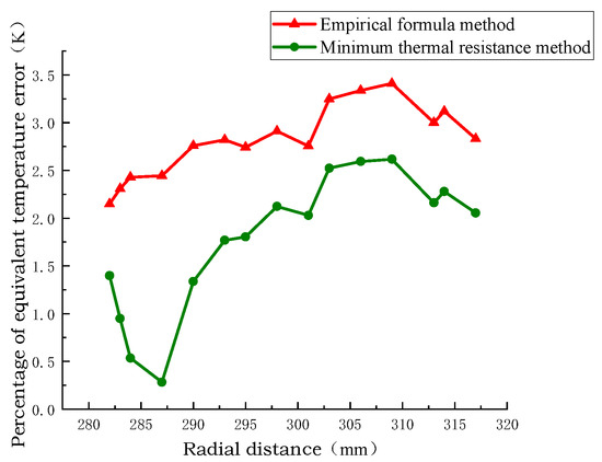
Figure 12. Comparison of models with radial temperature error of coil no.1.

As shown in Figure 13, Figure 14 and Figure 15. These results demonstrate that the equivalent model developed using the minimum thermal resistance method exhibits higher accuracy and reliability in temperature field simulation. It provides a more faithful representation of the actual temperature distribution within the winding structure, thereby validating its suitability for transformer thermal analysis.

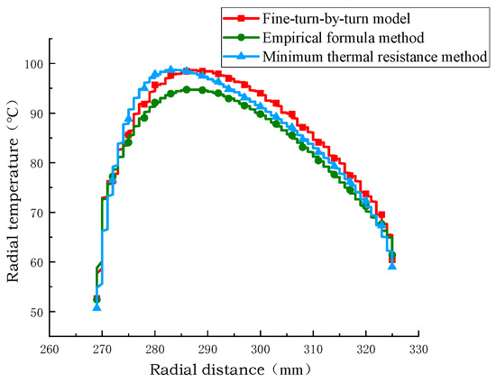
Figure 13. Comparison of radial temperature of coil no.2.

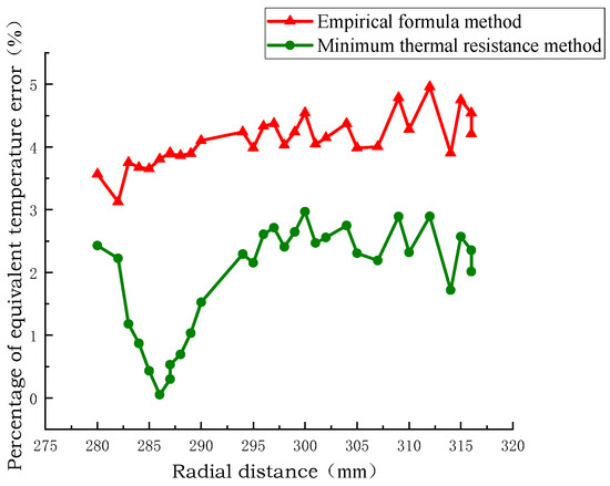
Figure 14. Comparison of the percentage of radial temperature error of the coil no.2.

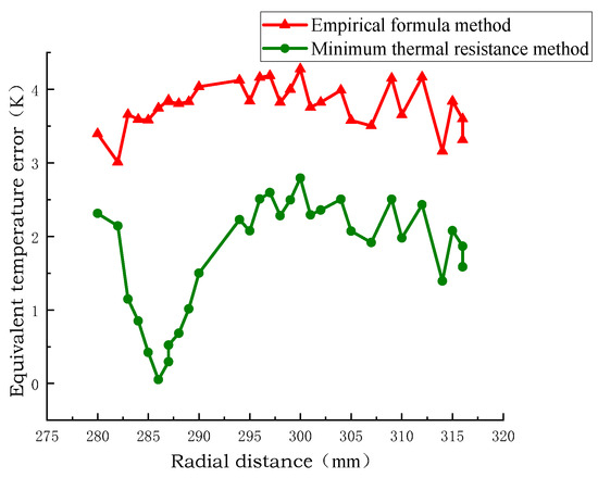
Figure 15. Comparison of the absolute value of the radial error of the coil no.2 between models.

The simulation results of the temperature at the axial centerline calculated by extracting the turn model, the empirical formula equivalent model, and the minimum thermal resistance equivalent model are shown in Figure 16, Figure 17 and Figure 18. In the direction of the axial vertical centerline, the hot spot position is the same, and the temperature of the winding disk increases with the increase in axial height. The axial temperature of the equivalent model of the minimum thermal resistance method is closer to that of the equivalent model of the empirical formula method and the temperature of the sub-turn model considering inter-turn insulation, and the axial temperature error of the equivalent model of the minimum thermal resistance method is 0.5 °C and 2.5 °C. The minimum percentage of axial temperature error is 1%, and the maximum percentage of error is 4%. This shows that the minimum thermal resistance method equivalent model has higher accuracy and reliability in simulating the axial temperature distribution of transformer windings.

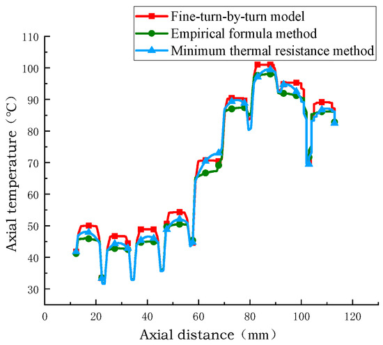
Figure 16. Comparison of axial temperatures calculated by different models.

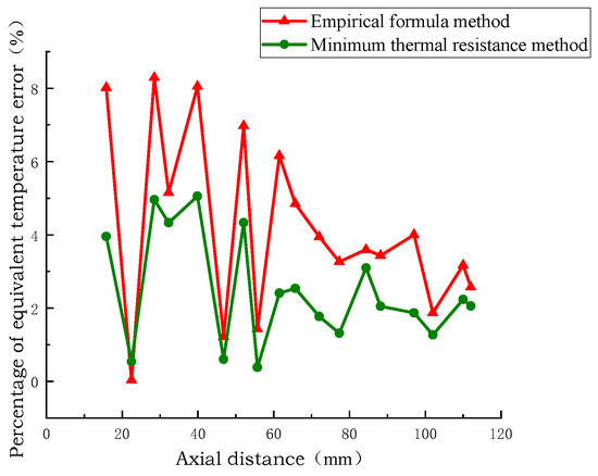
Figure 17. Comparison of axial temperature error percentage.

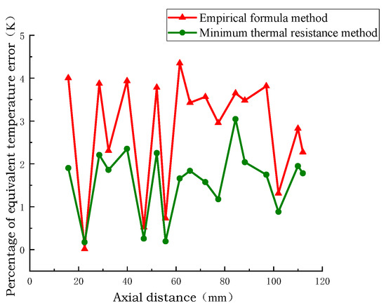
Figure 18. Axial distance temperature error.

5. Pilot Prototype Verification

Figure 19 shows the photo of the test transformer. The test adopts the equivalent test method of short-circuit wiring, the test time is 14 h, and the stability time is 4 h. The total loss of 65 kW should be added during the test, and the total loss of 65.6 kW should be applied. Windings temperature rise measurement: the specified current of 132.6 A should be added during the test, and the actual applied current should be 132.86 A. After the temperature rise in the windings was stabilized, the average temperature of the high-voltage winding was 84.8 °C, and the average temperature of the low-voltage windings was 85.5 °C. The average temperature rise in the high-voltage windings is 58.7 K, and the average temperature rise in the low-voltage windings is 59.4 K.

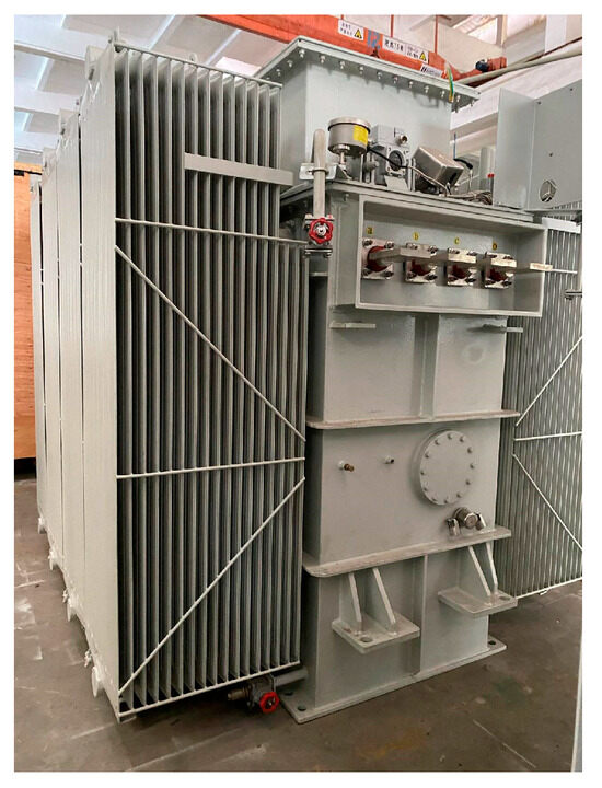
Figure 19. S7200KVA test prototype.

Using the equivalent thermal conductivity calculation method based on the law of minimum thermal resistance, the equivalent pre-turn windings of Figure 20 are equivalent to the windings disk shown in Figure 21, the material properties of the windings disk are set to copper, and the physical properties of the oil baffle and transformer oil are the same as those above.

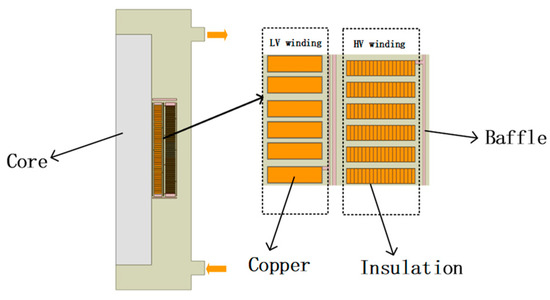
Figure 20. Actual 2D model.

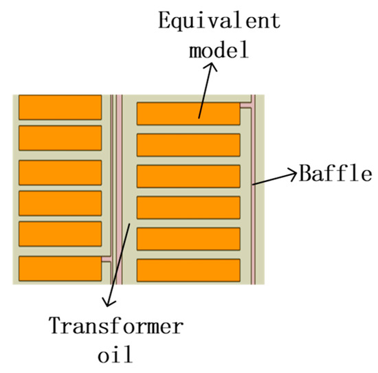
Figure 21. Equivalent post-2D model.

The calculated axial equivalent thermal conductivity of the high-voltage windings is 1.898 W/(m·K). The radial equivalent thermal conductivity is 0.444 W/(m·K). The axial equivalent thermal conductivity of the low-pressure windings is 5.48 W/(m·K). The radial equivalent thermal conductivity is 17.29 W/(m·K). The axial equivalent thermal conductivity of the high-voltage windings calculated by the empirical formula method is 10.29 W/(m·K). The radial equivalent thermal conductivity is 1.82 W/(m·K). The axial equivalent thermal conductivity of the low-pressure windings is 6.1 W/(m·K). The radial equivalent thermal conductivity is 18.2 W/(m·K).

The lower inlet of the axisymmetric model is set to the velocity and temperature boundary conditions, and the velocity direction is 0.0022 m/s, perpendicular to the inlet direction, which is equivalent to the actual outer radiator inlet area. The temperature is 300 K. The heat sources of the high-voltage windings and the low-voltage windings are shown in the table below. The outlet is set to the pressure boundary condition. The physical properties of each component are still set above, and the radial axial thermal conductivity of the windings is equivalent to the minimum thermal resistance method and the empirical formula method, respectively.The losses of the windings and the loss density are shown in Table 3.

Table 3. Heat sources of high- and low-voltage windings.

	Loss/W	Loss Density/W·m−3
High-voltage windings	23,703	189,624
Low-voltage windings	23,295	300,968

As can be seen from Figure 22 and Figure 23, a comparison between the equivalent thermal model based on the minimum thermal resistance method and that derived from the empirical formula method reveals that the former yields temperature field distributions more consistent with actual experimental measurements. Specifically, the experimental average temperature rises in the test prototype were measured to be 58.7 K for the high-voltage (HV) winding and 59.4 K for the low-voltage (LV) winding.

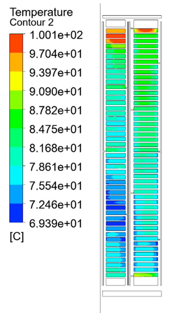
Figure 22. Temperature rise distribution of the equivalent model of the minimum thermal resistance method.

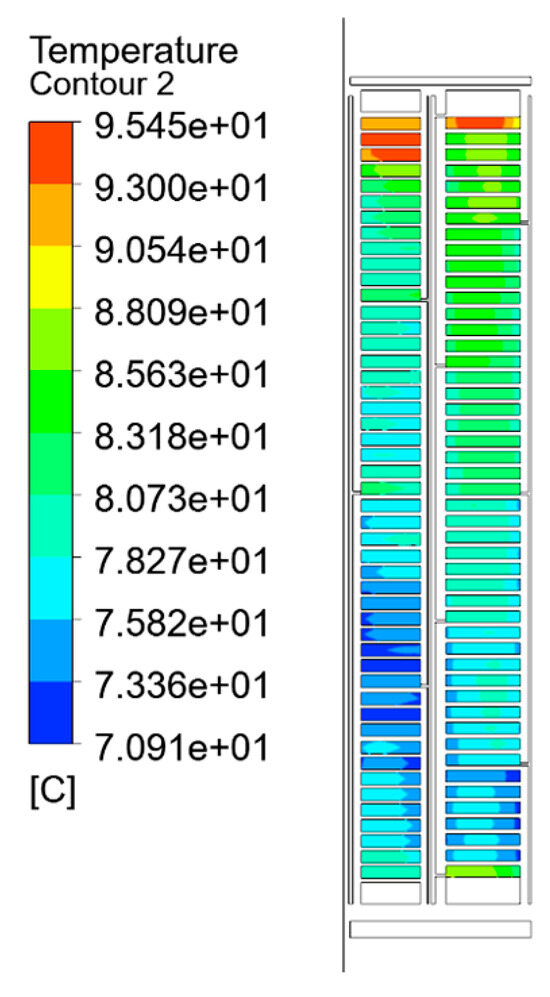
Figure 23. Temperature rise distribution of the empirical formula method equivalent model.

As can be seen from Table 4, In comparison, the equivalent model using the minimum thermal resistance method predicted an average temperature rise of 56.0 K for the HV winding, deviating from the experimental value by 2.7 K, and 58.21 K for the LV winding, with a deviation of 1.19 K. On the other hand, the empirical formula-based equivalent model resulted in an average temperature rise of 52.0 K for the HV winding, showing a larger discrepancy of 6.7 K, and 57.2 K for the LV winding, with a deviation of 2.2 K.

Table 4. Average and experimental temperatures of each model.

	High Voltage Windings Temperature Rise/K	Low Voltage Windings Temperature Rise/K
Minimum thermal resistance method equivalent model	56 (4.5%)	58.21 (2%)
Pilot prototype	58.7	59.4
Empirical formula method equivalence model	54 (8%)	57.2 (3.7%)

These discrepancies between simulation and experimental results may be attributed to several factors, including measurement uncertainties from temperature sensors, slight variations in operational conditions during experiments, and assumptions in the thermal modeling approach. Nevertheless, the results demonstrate that the minimum thermal resistance method offers superior accuracy over the empirical formula method in predicting the temperature rise in both HV and LV windings.

6. Conclusions

In order to solve the problem of large modeling workload and high computational cost when accurately calculating the temperature rise and hot spot of transformer windings, the equivalent thermal conductivity calculation method based on the law of minimum thermal resistance is given according to the principle of heat transfer, and the effectiveness of the calculation of temperature rise and hot spot is verified for the oil-immersed transformer windings model, and the calculation results show the following:

Under the condition of satisfying the actual requirements of the project, the number of meshes is 9831 when considering the fine modeling of inter-turn insulation, while the number of meshes is 3453 when the equivalent thermal conductivity method is used, and the number of meshes is reduced by 65%.

By synthesizing the temperature field simulation results of the proportional turn model, the equivalent model based on the minimum thermal resistance method, and the equivalent model of the empirical formula method, it can be concluded that the hot spot positions of the equivalent model of the minimum thermal resistance method are basically consistent with those of the model before equivalence. In addition, in terms of the average temperature and hot-spot temperature of each winding disk, the error of the equivalent model of the minimum thermal resistance method is smaller than that of the equivalent model of the empirical formula method, which verifies the accuracy of the equivalent thermal conductivity method. At the same time, in the comparison with the temperature rise test results of the prototype, the calculation results of the equivalent model based on the minimum thermal resistance method are closer to the test values, and it is more accurate in reflecting the actual temperature rise distribution than the equivalent model of the empirical formula method.

References

- Zhang, H.; Wang, L.; Chen, X.; Li, Y. Improved information entropy weighted vague support vector machine method for transformer fault diagnosis. High Volt. 2022, 7, 510–522. [Google Scholar] [CrossRef]
- Darwish, M.M.F.; Abdelhalim, A.; Ibrahim, S.; El-Hagry, M.T. A new technique for fault diagnosis in transformer insulating oil based on infrared spectroscopy measurements. High Volt. 2024, 9, 319–335. [Google Scholar] [CrossRef]
- Zhou, L.; Yuan, S.; Zhu, Q.; Wang, D.; Wang, L. Transient thermal network model for train-induced wind cooling dry-type on-board traction transformer in electric multiple units. High Volt. 2023, 8, 514–526. [Google Scholar] [CrossRef]
- Kuhn, G.G.; Sousa, K.M.; Martelli, C.; Bavastri, C.A.; Silva, J.C.C.D. Embedded FBG Sensors in Carbon Fiber for Vibration and Temperature Measurement in Power Transformer Iron Core. IEEE Sens. J. 2020, 20, 13403–13410. [Google Scholar] [CrossRef]
- Wu, T.; Yang, F.; Farooq, U.; Jiang, J.; Hu, X. Real-time calculation method of transformer winding temperature field based on sparse sensor placement. Case Stud. Therm. Eng. 2023, 47, 103090. [Google Scholar] [CrossRef]
- Oliveira, M.M.; Medeiros, L.H.; Kaminski, A.M.; Falcão, C.E.G.; Beltrame, R.C.; Bender, V.C.; Marchesan, T.B.; Marin, M.A. Thermal-hydraulic model for temperature prediction on oil-directed power transformers. Int. J. Electr. Power Energy Syst. 2023, 151, 109133. [Google Scholar] [CrossRef]
- Wang, L.; Dong, X.; Jing, L.; Li, T.; Zhao, H.; Zhang, B. Research on digital twin modeling method of transformer temperature field based on POD. Energy Rep. 2023, 9, 299–307. [Google Scholar] [CrossRef]
- Chen, Q.; Chen, S.; Huang, W.; Zhang, W.; Li, K. Research on Inversion Model of Winding Hot Spot Temperature of 10-kV Oil-Immersed Three-Dimensional Coiled Core Transformer. IEEE Access 2024, 12, 97691–97700. [Google Scholar] [CrossRef]
- Radakovic, Z.; Jovcic, D.; Nedeljkovic, M. Ratings of oil power transformer in different cooling modes. IEEE Trans. Power Deliv. 2012, 27, 618–625. [Google Scholar] [CrossRef]
- Bhardwaj, R.G.; Khare, N. Review: 3-ω Technique for Thermal Conductivity Measurement—Contemporary and Advancement in Its Methodology. Int. J. Thermophys. 2022, 43, 139. [Google Scholar] [CrossRef]
- Sliwa, T.; Leśniak, P.; Sapińska-Śliwa, A.; Rosen, M.A. Effective thermal conductivity and borehole thermal resistance in selected borehole heat exchangers for the same geology. Energies 2022, 15, 1152. [Google Scholar] [CrossRef]
- Yang, G.; Cao, B.Y. Three-sensor 2ω method with multi-directional layout: A general methodology for measuring thermal conductivity of solid materials. Int. J. Heat Mass Transf. 2024, 219, 124878. [Google Scholar] [CrossRef]
- Zhang, M.; Bi, J.; Chen, W.; Zhang, X.; Lu, J. Evaluation of calculation models for the thermal conductivity of soils. Int. Commun. Heat Mass Transf. 2018, 94, 14–23. [Google Scholar] [CrossRef]
- Wejrzanowski, T.; Grybczuk, M.; Chmielewski, M.; Pietrzak, K.; Kurzydlowski, K.J.; Strojny-Nedza, A. Thermal conductivity of metal-graphene composites. Mater. Des. 2016, 99, 163–173. [Google Scholar] [CrossRef]
- Li, Z.; Yang, Y.; Gariboldi, E.; Li, Y. Computational models of effective thermal conductivity for periodic porous media for all volume fractions and conductivity ratios. Appl. Energy 2023, 349, 121633. [Google Scholar] [CrossRef]
- Zhan, C.; Cui, W.; Li, L. A fractal model of effective thermal conductivity of porous materials considering tortuosity. Energies 2023, 16, 271. [Google Scholar] [CrossRef]
- Taheri, A.A.; Abdali, A.; Rabiee, A. A novel model for thermal behavior prediction of oil-immersed distribution transformers with consideration of solar radiation. IEEE Trans. Power Deliv. 2020, 34, 1634–1646. [Google Scholar] [CrossRef]
- Ai, M.; Shan, Y. The whole field temperature rise calculation of oil-immersed power transformer based on thermal network method. Int. J. Appl. Electromagn. Mech. 2022, 70, 55–72. [Google Scholar] [CrossRef]
- Dey, A.; Shafiei, N.; Li, R.; Eberle, W.; Khandekar, R. Boundary Condition Independent Thermal Network Modeling of High-Frequency Power Transformers. Heat Transf. Eng. 2023, 44, 259–276. [Google Scholar] [CrossRef]
- Radakovic, Z.; Jevtic, M.; Das, B. Dynamic thermal model of kiosk oil immersed transformers based on the thermal buoyancy driven air flow. Int. J. Electr. Power Energy Syst. 2017, 92, 14–24. [Google Scholar] [CrossRef]
Disclaimer/Publisher’s Note: The statements, opinions and data contained in all publications are solely those of the individual author(s) and contributor(s) and not of MDPI and/or the editor(s). MDPI and/or the editor(s) disclaim responsibility for any injury to people or property resulting from any ideas, methods, instructions or products referred to in the content. |
© 2025 by the authors. Licensee MDPI, Basel, Switzerland. This article is an open access article distributed under the terms and conditions of the Creative Commons Attribution (CC BY) license (https://creativecommons.org/licenses/by/4.0/).