Article

Milepost-to-Vehicle Monocular Depth Estimation with Boundary Calibration and Geometric Optimization

by
Enhua Zhang
,
Tao Ma
,
Handuo Yang
,
Jiaqi Li
,
Zhiwei Xie
and
Zheng Tong
*
School of Transportation, Southeast University, Nanjing 210096, China
*
Author to whom correspondence should be addressed.
Electronics 2025, 14(17), 3446; https://doi.org/10.3390/electronics14173446
Submission received: 22 July 2025 / Revised: 20 August 2025 / Accepted: 22 August 2025 / Published: 29 August 2025
(This article belongs to the Section Electrical and Autonomous Vehicles)

Abstract

Milepost-assisted positioning estimates the distance between a vehicle-mounted camera and a milepost as a reference position for autonomous driving. However, the accuracy of monocular metric depth estimation is compromised by camera installation angle, milepost inclination, and image occlusions. To solve the problems, this paper proposes a two-stage monocular metric depth estimation with boundary calibration and geometric optimization. In the first stage, the method detects a milepost in one frame of a video and computes a metric depth map of the milepost region by a monocular depth estimation model. In the second stage, in order to mitigate the effects of road surface undulation and occlusion, we propose geometric optimization with road plane fitting and a multi-frame fusion strategy. An experiment using pairwise images and depth measurement demonstrates that the proposed method exceeds other state-of-the-art methods with an absolute relative error of 0.055 and root mean square error of 3.421.

1. Introduction

Mileposts provide the mileage information between a current location and a road starting point. Milepost-assisted localization technology estimates the distance between a vehicle and a milepost, offering reliable mileage references for constructing and updating high-precision maps in autonomous driving systems. For instance, global navigation satellite system (GNSS) signals may be obstructed or disrupted in a mountainous area, leading to inaccurate navigation positioning. In such scenarios, the integration of a milepost coordinate and the relative positions between the milepost and a vehicle can guarantee localization accuracy.
Milepost-assisted positioning technologies can be categorized into three directions: the matching between map and road features, the multi-sensor fusion, and the global position system (GPS) and image fusion. The first direction aligns high-precision maps with road features (e.g., lane markings and traffic signs) to assist positioning [1,2,3], offering high accuracy and requiring minimal hardware resources. However, the high cost of constructing and updating high-precision maps limits their application, especially in areas with indistinct road features.
The second direction integrates position data from multiple sources, including GPS, inertial navigation systems (INS), vision sensors, and odometry, achieving millimeter-level positioning accuracy [4,5]. Though this direction provides superior precision, it heavily relies on high-performance hardware. Specifically, the reliability of the direction decreases in cases of sensor failure or extreme terrains.
The final direction utilizes onboard cameras to capture video or images, extracting the location information of mileposts through object detection, which are then combined with GPS coordinates for precise positioning [6,7]. However, there is a distance deviation between the onboard camera and the milepost due to their non-parallel alignment in the third step in Figure 1. The existing solutions primarily involve adjusting the camera installation angle for compensation. The uncertainty of the location of the mileposts and the fixed camera angle may lead to the omission of the targets. Furthermore, onboard cameras need to capture road features ahead, and adjusting the angle for milepost detection may weaken the detection of other objects, reducing coverage and overall task efficiency.
To address the problem of depth estimation in milepost-assisted positioning, this paper proposes a two-stage monocular metric depth estimation method with boundary calibration and geometric optimization. In the first stage, an unsupervised monocular depth estimation network is first employed to generate a relative depth map. A scale recovery module based on a lower field-of-view road boundary is then introduced during the post-processing phase to convert the relative depth into a metric depth map. Subsequently, the milepost region is identified using an object detection algorithm, and its average metric depth is extracted as the initial estimate of the camera-to-milepost distance. In the second stage, a road plane is fitted using SVD and RANSAC, and the milepost depth is projected along the road longitudinal direction to correct errors caused by camera installation angle and milepost inclination. Finally, a multi-frame geometric fusion module aligns and fuses depth information from adjacent frames to obtain a final depth result. An experiment with 352 real-world samples is used to demonstrate the effectiveness of the proposed method. The main contributions of this study can be summarized as follows:
(a) The proposed monocular metric depth estimation method achieves superior performance compared to existing metric depth prediction-based and relative depth scaling-based approaches, while maintaining stable results under various real-world conditions such as different distance ranges, illumination, and road surfaces.
(b) By leveraging the lower field-of-view road boundary, the proposed scale recovery module effectively resolves the inherent scale ambiguity in monocular depth estimation. In the first stage, a scale recovery module based on the lower field-of-view road boundary effectively resolves the inherent scale ambiguity in monocular depth estimation, enabling accurate metric depth recovery.
(c) Road-plane-based geometric optimization mitigates depth estimation errors caused by non-parallel camera installation and milepost inclination, while multi-frame geometric fusion enhances robustness against occlusions and illumination variations.

2. Related Works

Research on monocular depth estimation has achieved remarkable progress in recent years, with numerous approaches proposed to enhance depth accuracy and robustness under complex scenarios. At the same time, how to recover a reliable metric scale from inherently relative depth predictions remains a critical challenge. In this section, we first review representative approaches to monocular depth estimation, and then summarize scale recovery algorithms that are particularly relevant to our work.

2.1. Monocular Depth Estimation

Monocular depth estimation predicts the depth information of an object in a single image. In recent years, deep learning methods have achieved significant success in this field.
Supervised learning-based methods rely on large-scale training datasets with ground-truth depth labels for model optimization. Eigen et al. [8] were the first to employ a convolutional neural network (CNN) architecture for depth estimation; this method pioneered the use of neural networks in this field. Subsequently, numerous studies have significantly improved depth estimation accuracy and detail preservation by enhancing network architectures [9,10,11] or introducing novel optimization strategies [12,13]. However, these methods are highly dependent on large-scale, high-quality depth-annotated datasets, which are costly and labor-intensive to acquire.
Semi-supervised learning-based methods train models by leveraging a small amount of labeled data along with a large amount of unlabeled data. It can reduce dependence on depth-annotated datasets. These methods typically incorporate 3D LiDAR data [14], semantic information [15,16], stereo disparity maps [17] or optical flows [18] as auxiliary supervision signals to improve depth estimation accuracy. However, semi-supervised learning-based methods involve complex loss function designs and hyperparameter tuning, which increase the difficulty of model training while also imposing higher computational resource requirements.
Unsupervised learning-based monocular depth estimation methods require only an image sequence as input during training. It is beneficial for eliminating the need for ground-truth depth labels. Early approaches can be categorized into image pair-based training [19] and image sequence-based training [20]. The former reconstructs images using disparity maps, employing reconstruction error as the supervision signal, while the latter jointly estimates camera pose and depth information to address the scale ambiguity problem. Subsequent studies have improved depth prediction accuracy and robustness in complex scenes by optimizing network architectures [21,22]. Additionally, recurrent depth estimation models [23] and continual learning frameworks [24] have further enhanced the adaptability and generalization capability in dynamic environments. By leveraging weather-related augmentations together with a pseudo-supervised loss for depth and pose, Robust-Depth effectively addressed the challenging conditions such as nighttime, fog, and rain [25]. However, unsupervised learning methods often feature complex network structures, leading to increased inference time and higher memory consumption.

2.2. Monocular Depth Estimation Scale Recovery Algorithms

Monocular metric depth estimation can be understood as a problem of depth ranking and depth scale recovery [26]. Due to the lack of multi-view information and scene geometric constraints, monocular cameras provide only relative depth estimates, leading to the scale ambiguity problem. Depth scale recovery refers to the process of converting the relative depth obtained from relative depth into metric depth.
Currently, depth scale recovery methods can be broadly categorized into two main approaches. The first approach involves directly predicting metric depth using monocular depth estimation models. Zero-shot methods [27,28,29,30,31] train models on a source dataset and directly apply them to a target dataset without requiring specific camera intrinsics or prior scene knowledge. These methods can output metric depth values for arbitrary unknown environments. They rely on strong geometric consistency across domains, making them sensitive to domain shifts. Weakly supervised methods incorporate non-depth information (e.g., GPS [32], velocity [33], surface normal [34], LiDAR [35], scene semantics [36] and virtual-SfM signals [37] as auxiliary supervision signals to refine the metric depth scale. MonoPP leverages monocular video and known camera mounting geometry using planar-parallax reconstruction to achieve self-supervised metric-scaled depth predictions [38]. While these methods reduce reliance on dense depth labels, they require high-quality sensor data, making them heavily dependent on hardware capabilities. Hybrid supervision methods combine synthetic and real-world data, using style transfer techniques [39,40] to enhance model adaptability. PatchRefiner refines high-resolution metric depth using a tile-based architecture and a detail-and-scale disentangling loss, achieving strong performance across synthetic and real-world datasets [41]. However, the distribution gaps between synthetic and real-world data lead to limited generalization performance, reducing the effectiveness of models in real-world scenarios.
The second method estimates relative depth using a monocular depth estimation model. Then they calculate a scale factor between the relative and metric depth values to achieve scale recovery. Zhang et al. [42] utilized pose data from navigation sensors and applied a multi-view geometric model to compute the scale factor between relative and metric depth. Masoumian et al. [43] employed curve fitting techniques to establish a mapping between relative depth values and known ground-truth depth values, optimizing the scale factor using least squares minimization. However, this method requires extensive real-world depth data and assumes a uniform and diverse data distribution. Dana et al. [44] proposed a field-of-view correction method, adjusting the source dataset’s FoV to match the target dataset, and then computing a depth correction scale factor using the ground-truth depth from the source dataset. This method is effective for FoV discrepancies but struggles with more complex geometric domain shifts. Zhu et al. [45] decomposed metric depth estimation into scene scale prediction and relative depth estimation, improving scale recovery accuracy. McCraith et al. [46] and Xue et al. [47] utilized known camera height and estimated road plane distances to compute the scale factor. Yang et al. [48] further introduced a frame buffering algorithm, using adjacent frames to optimize ground point sets, reducing the impact of noisy points in single-frame images on depth correction. Although this method mitigates scale bias, it still relies on ground-truth depth data to compute the scale factor. To address these limitations, we propose a multi-frame depth scale recovery method based on boundary calibration and geometric fusion. The proposed method eliminates the need for extensive real-world depth data, complex model training, and hardware-dependent constraints, providing a more practical and efficient solution for monocular metric depth estimation.

3. Methodology

3.1. Overview

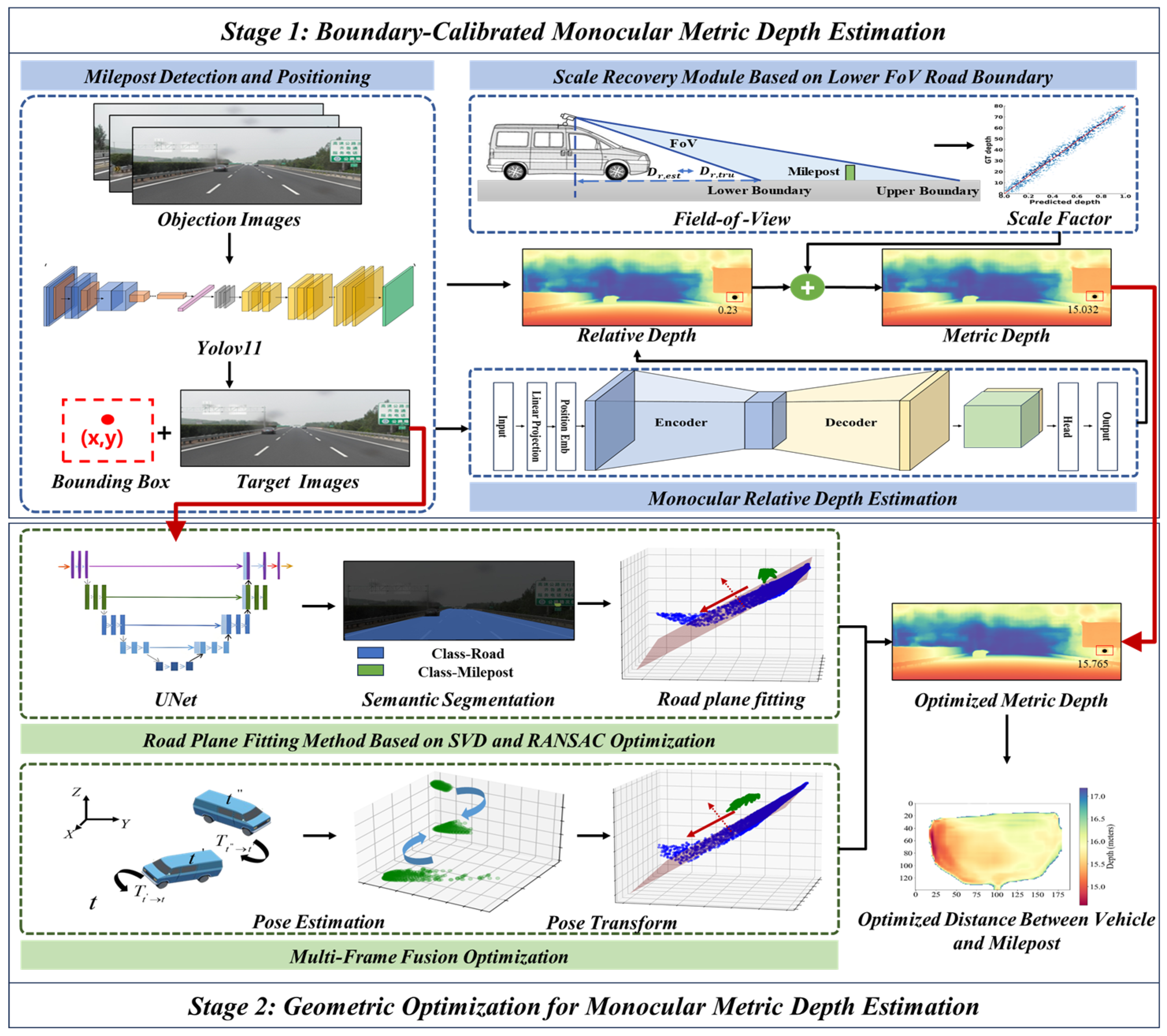
This paper proposes a two-stage monocular metric depth estimation with boundary calibration and geometric optimization to estimate the distance between a vehicle and a milepost. The procedure can be summarized in the following steps, as shown in Figure 2.
In Stage 1, a boundary-calibrated monocular metric depth estimation model is proposed to generate a metric depth map. This stage consists of Section III (B), III (C), and III (D). The model first utilizes an unsupervised monocular depth estimation network to predict a relative depth map from the input image. The monocular depth estimation network will be introduced in Section III (B). Subsequently, a scale recovery module based on a lower field-of-view road boundary is introduced as a post-processing step. The road lower boundary is a line of pixels at the bottom of the image, such as the red one in Figure 3 The average depth along this boundary is used to compute a global scale factor. The global scale factor transforms the relative depth map into the metric depth map. The detailed implementation of the scale recovery process is described in Section III (C). Finally, a YOLOv11 object detection algorithm [49] is applied to locate the milepost region, from which the average metric depth value is extracted as the initial estimate of the distance between the vehicle and the milepost. The detailed procedure for milepost detection and image coordinate extraction based on YOLOv11 is presented in Section III (D).
In Stage 2, to further optimize the initial metric depth, a geometric optimization process is introduced. This stage consists of Section III (E) and III (F). First, a road longitudinal direction vector is computed by a road plane fitting method based on value decomposition (SVD) and random sample consensus (RANSC). The road longitudinal direction vector is used to optimize the metric depth map from Stage 1, avoiding the negative effects of the camera installation angle and milepost inclination. Thus, an optimized metric depth map is obtained. The details of the road plane fitting model are described in Section III (E). Considering that the milepost region in certain frames may be occluded or unclear, which could lead to inaccurate depth estimation, a multi-frame fusion strategy is applied. The strategy first computes the frame-by-frame pose transformation matrices by the pose estimation. The pose transformation matrices then convert the optimized metric depth maps of adjacent frames from Section III (E) into the coordinate system of the current frame if the occluded and unobvious exist. Next, the metric depth maps in the same coordinate system are integrated by a weighted averaging method. Finally, the optimized metric depth of the milepost is output as the distance between the vehicle and the milepost. The multi-frame fusion models are described in Section III (F).

3.2. YOLOv11-Based Milepost Detection and Positioning

YOLOv11 [49] is the latest generation of object detection algorithm released by Ultralytics in September 2024. Its overall architecture consists of three main components: the backbone, the neck, and the detection head. The backbone is responsible for extracting image features and mainly includes the Conv module, C3K2 module, SPPF module, and C2PSA module. The detection head performs the final object detection tasks. It supports higher input resolutions with minimal latency and provides stronger small-object detection capability, making it well-suited for distant mileposts under varying illumination and occlusion. In this study, an improved version of the YOLO v11 algorithm is adopted to automatically detect and localize milepost targets in road scene images.
To construct a reliable dataset for YOLO v11 training, a large number of road front-view images were collected from highways across multiple regions, including Shandong and Jiangsu provinces, using a multifunctional detection vehicle. Among these, images containing visible milepost targets were manually selected. Each selected image was annotated with bounding boxes to label the position of the milepost, resulting in a labeled dataset for supervised learning. A total of 2547 annotated images were prepared and split into training, validation, and test sets in a ratio of 7:2:1, yielding 1783 training images, 509 validation images, and 244 test images. This dataset serves as the foundation for training and evaluating the YOLOv11 model, ensuring its robustness and generalization under diverse road scenarios.
The trained YOLOv11 model is applied to the input image sequence in a frame-by-frame manner to automatically identify the presence of milepost targets and output their bounding box coordinates in the image plane. These detection results are used to locate the corresponding milepost regions in the monocular metric depth maps. By mapping the bounding box coordinates onto the depth map, the depth values within the detected regions can be effectively extracted. Subsequently, the average depth value within the region is computed to provide an initial estimate of the distance between the camera and the milepost.

3.3. Unsupervised Learning Monocular Relative Depth Estimation Model

In this section, the milepost region is converted into a relative depth map using the model, where the relative depth provides a depth reference for metric depth optimization. Figure 4 presents the network architecture of the unsupervised learning monocular relative depth estimation model, which integrates a vision transformer-large (ViT-L) as the encoder and a dense prediction transformer (DPT) as the decoder.
The ViT-L encoder consists of 24 transformer layers, learning the global contextual information related to scene structure, object boundaries, depth relationships, and spatial coherence effectively. The encoder extracts multi-scale features from the 6th, 12th, 18th, and 24th transformer layers, capturing a hierarchy from high-resolution edge details at shallow layers to low-resolution semantic features at deeper layers. These multi-scale features are directly passed to the decoder through skip connections, ensuring semantic consistency while refining depth estimation details. The DPT decoder further processes these features to reconstruct a high-quality relative depth map, maintaining both fine-grained depth details and global scene understanding.
The DPT decoder restores the feature resolution through progressive upsampling. The decoder fuses the current feature map with the corresponding encoder feature map, ensuring effective utilization of multi-level information. The decoder improves the clarity of depth map details by incorporating low-level edge information. At the same time, it preserves semantic completeness by integrating high-level global features. Finally, a fully connected convolutional layer maps the high-dimensional feature representation into a single-channel depth map. Each pixel value in this map corresponds to the relative depth of the point in the scene.
The model training process consists of two stages: teacher model training and student model training. In the teacher model training stage, the model is trained by a dataset of 595 K high-quality synthetic images, covering a wide range of scenes and complex layouts while providing precise depth supervision. Multiple loss functions are employed to optimize depth prediction, ensuring robustness across different conditions. These loss functions are derived from the methods described in [50]. The scale-shift invariant loss L s s i is used to maintain consistent in-depth predictions under varying scales and shifts. The loss function can be calculated as
L s s i = 1 N i = 1 N l o g d i ^ l o g d i 2 1 N i = 1 N l o g d i ^ l o g d i 2 ,
where N denotes the number of pixels used for loss computation, d i ^ is the predicted depth values and d i represents the ground truth depth values.
The gradient matching loss L g m is employed to enhance the sharpness of depth boundaries. The loss function can be calculated as
L g m = 1 N i = 1 N x d i ^ x d i 2 + y d i ^ y d i 2 ,
where x and y represent the gradient computed in the horizontal and vertical depth variation.
In the student model training stage, the teacher model is first used to generate pseudo-depth labels for 62 M unlabeled real-world images. These high-quality pseudo labels are then leveraged to train the student model, further enhancing its generalization capability in real-world scenarios. To ensure that the feature representations of the student model remain aligned with those of the teacher model, a feature alignment loss L a l i g n is introduced during training. The loss function can be calculated as
L a l i g n = 1 N i = 1 N F s x i F t x i 2 ,
where F s x i and F t x i represent the feature representations of the student model and teacher model at pixel x i .

3.4. Scale Recovery Module Based on Lower Field-of-View Road Boundary

The relative depth maps in Section III (B) require a reference for metric depth conversion. The proposed depth calibration model uses the distance between the camera and the boundary of the road surface at the bottom boundary as the reference since the distance is fixed and can be pre-measured once the camera is fixed in a vehicle, as shown in the red dashed line of Figure 3. The relative depth maps in Section III (B) can be recovered into the metric depth map using the known depth information at the field-of-view boundary, without requiring additional calibration procedures.
The depth calibration model first obtains the road surface points in the low boundary region of the camera view field. A U-Net network is adopted to obtain the surface points in the input frame. Let the semantic segmentation result of the input frame be denoted as S u , v . If the prediction class of a pixel is road surface, the set of road surface pixels p r as
p r = u , v | S u , v = l r ,
where u , v represents the 2D coordinates of a pixel, l r represents the road class label.
The road surface pixels in the low boundary region of the camera view can be refined by selecting pixels from the last row of the frame. The set of road pixels in the bottommost row p b can be calculated as
p b = u , v p r | v H 1 , H ,
where H is the frame height. Equation (5) selects only those road pixels whose vertical coordinate v lies in the last row of the frame, ensuring that only the pixels at the lower boundary of the camera’s field of view are considered.
The depth value set the field-of-view boundary road pixels D b for the FoV boundary road pixels is defined based on the selected boundary pixel set p b as
D b = D u , v | u , v p b ,
where D u , v represents the relative depth value at the pixel u , v .
The median depth of the field-of-view boundary road is computed to obtain the preliminary estimation of the road surface D r , e s t as
D r , e s t = m e d i a n D b .
Subsequently, a scaling relationship between the true depth and the estimated depth is established by conducting a real-world measurement of the true metric depth between the onboard camera and the field-of-view boundary road region. The depth scale factor f is defined as
f = D r , t r u / D r , e s t ,
where D r , t r u represents the measured metric depth of the road at the field of view boundary.
Using the depth scale factor calibration formula, all relative depth values in the depth map are initially converted into metric depth values D a b u , v as
D a b u , v = f D r e l u , v ,
where D r e l u , v represents the relative depth at the pixel u , v in the relative depth map.

3.5. Road Plane Fitting Method Based on SVD and RANSAC Optimization

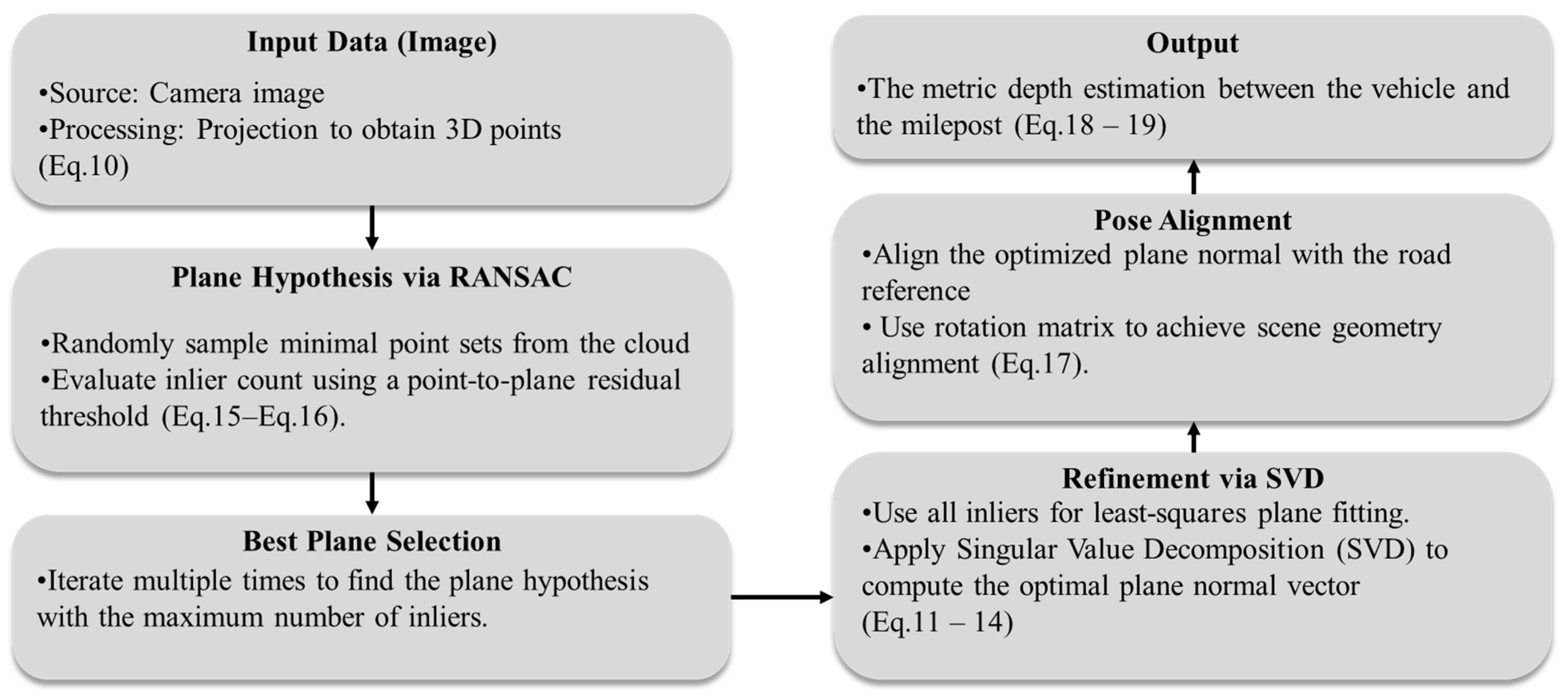
The depth estimation in Equation (9) may deviate from the actual distance owing to the effects of the camera installation angle and milepost inclination, as shown in Figure 5. Since the road plane serves as a crucial geometric reference for the vehicle-camera relationship, its plane normal vector can be transformed into a longitudinal directional vector along the road, providing geometric constraints between the vehicle and the milepost. However, the road surface point cloud used for plane fitting contains a significant amount of noise points. This study incorporates SVD and RANSAC for iterative optimization, filtering out outliers, and refining both the plane normal vector and the longitudinal directional vector in Figure 6. This optimization provides a reliable geometric reference for subsequent depth projection and scale recovery.
First, by using the intrinsic parameters of the camera and the depth map, the set of road pixels obtained in Section III (C) is projected into 3D space. The road pixel set is transformed into a 3D point cloud P i r as
P i r = K 1 D a b u , v u v 1 ,   u , v p r ,
where K is the camera intrinsic matrix.
Before performing road plane fitting, the number of 3D road surface points is first evaluated. If the number of road surface points is less than 3, it indicates that “No Valid Road Information Exists”, making plane fitting infeasible. If the number of points is greater than or equal to 3, the road plane fitting process proceeds. Next, the initial parameters for the RANSAC algorithm are defined, including the inlier threshold ε . A point is considered an inlier if its distance to the candidate plane is less than ε . Additionally, the maximum number of iterations N for RANSAC and the inlier ratio threshold r i n for early termination conditions are specified.
In each iteration, k points are randomly selected from the 3D point cloud P i r to form the sampling point set P s a m = P i 1 r , P i 2 r , , P i k r . The centroid of the sampling point set c is then computed as
c = 1 k j = 1 k P i j r ,
where k is the number of points sampled in each iteration, P i j r denotes the j -th of selected 3D point from the road point cloud.
After obtaining the centroid of the sampling point set, the offset matrix A is computed and subjected to SVD as
A = P i j r c j = 1 k
A = U V T
with the plane normal vector n as
n = V : , 1 / V : , 1 ,
where U is an N × N matrix whose column vectors are orthogonal, is an N × 3 diagonal matrix, with the singular values arranged in descending order, V is a 3 × 3 matrix whose column vectors are the right singular vectors of A . The last column vector of V , corresponding to the smallest singular value, represents the normal vector direction of n the fitted road plane.
Then the distance between the three-dimensional point set of the road and the candidate road plane is calculated as
D i = n P i r c / n .
For each point P i r , if the condition D i < ε is satisfied, the point is classified as an inlier, and all inliers are recorded in the inlier set P i n = P i r | D i < ε . During each iteration, the inlier ratio is computed as
r c u r = P i n / P i r o a d .
If r c u r > r i n or the maximum number of iterations N is reached, the iteration stops, and the optimized road plane equation and optimized normal vector n o p t are obtained. To further refine the depth estimation, a rotation matrix is introduced to transform the optimized road plane normal vector n o p t , into a direction vector along the road s r . Specifically, R is constructed to align the estimated normal vector with the global road coordinate system, ensuring that the recovered depth values are geometrically consistent with the actual road surface. The transformation is expressed as
s r = R × n o p t ,
where R is the rotation matrix aligning the estimated normal vector with the road direction; and n o p t is the optimized normal vector of the road plane.
The longitudinal direction vector along the road s r serves as the optimized depth projection direction, providing a stable geometric foundation for single-frame and multi-frame fused depth estimation. After obtaining the optimized projection direction vector s r , the semantic segmentation model trained in Section III (B) is used to infer the image and extract the milepost pixel set p m with category label l m . The set of milepost pixels is projected into the three-dimensional space to obtain the three-dimensional point cloud of the milepost P i m as
P i m = K 1 D a b u , v u v 1 , u , v p m ,
The point set of the milepost is projected along the vector s r and the average of the projected point set is taken as the depth after optimizing the current frame. The metric depth estimation between the vehicle and the milepost is obtained as D f _ s i n as
D f _ s i n = i = 1 W s r P i m / W ,
where W is the number of points in the milepost set.

3.6. Dynamic Single-Frame Computation and Multi-Frame Fusion Optimization

Due to occlusions and camera perspective limitations, the milepost point set in a single-frame image may not accurately reflect the true depth of the milepost. Directly computing the projection along the road longitudinal normal vector based on the milepost point set from a single frame as the optimized metric depth between the vehicle and the milepost may introduce errors. To address this issue, we propose a multi-frame fusion-based milepost point set optimization method, which integrates information from the current frame and the adjacent previous and next frames to compensate for missing milepost information caused by occlusions or viewpoint limitations in the current frame.
In the multi-frame fusion depth estimation process, to ensure the effectiveness of the fusion, it is necessary to verify that the current frame and its adjacent frames both contain valid milepost information. For frames t 1 , t and t + 1 , the semantic segmentation model is used to extract the milepost encodings p m , p r e , p m , c u r and p m , n e x . To determine whether a frame contains valid milepost information, the total number of mileposts encoding pixels p m is compared with the threshold as
V a l i d p m = T r u e ,     i f p m τ F a l s e ,     o t h e r w i s e ,
where V a l i d · is a Boolean function that determines whether the frame contains valid milepost encoding information. τ is a predefined threshold for the minimum required milepost encoding pixels to consider the frame as valid. Frames meeting this criterion are selected as valid frames for depth estimation.
To ensure the reliability of depth estimation, it is necessary to verify that the current frame and its neighboring frames simultaneously contain valid milepost mask information. This condition is satisfied when the validity function for all three frames returns True, which is expressed as
V a l i d p m , p r e V a l i d p m , c u r V a l i d p m , n e x ,
If the above conditions are not met, the system falls back to a single-frame computation mode. If the conditions are met, the multi-frame fusion mode is used to compute the metric depth between the vehicle and the milepost. To obtain the pose transformation matrix between the adjacent frames and the current frame, the oriented fast and rotated brief algorithm is used to detect key points in the images and generate descriptors. After detecting key points, the brute-force matcher is applied to match descriptors between adjacent frames, selecting the optimal matching pairs based on matching distance. Once the matched key points are obtained, the pose transformation matrices between adjacent frames are estimated. These matrices are then used to align the milepost point sets from the previous and next frames with the current frame’s coordinate system, as
P p r e _ c u r = T p r e _ c u r P | P ϵ P m , p r e P n e x _ c u r = T n e x _ c u r P | P ϵ P m , n e x ,
where P p r e _ c u r and P n e x _ c u r represent the transformed milepost point set from the previous and next frame to the current frame’s coordinate system, respectively. T p r e _ c u r and T n e x _ c u r are the estimated transformation matrices from the previous and next frame to the current frame, respectively. P m , p r e and P m , n e x denote the sets of milepost points extracted from the previous and next frames, respectively.
According to Equation (19), the projected depth values along the depth projection direction vector are computed for the transformed milepost point sets from different frames. The projected depth values D c u r , D p r e _ c u r and D n e x _ c u r are fused based on milepost occlusion, image quality, and other factors. The final multi-frame optimized metric depth estimation D f _ m u l between the vehicle and the milepost is computed as
D f _ m u l = w i D i w i , i pre_cur ,   c u r , nex_cur ,
where D c u r is the projected depth value from the current frame. D p r e _ c u r and D n e x _ c u r are the projected depth values from the previous and next frame, aligned with the current frame. w c u r , w p r e _ c u r and w n e x _ c u r are the weight coefficients for the current, previous, and next frames, respectively.
The pseudocode for the dynamic single-frame computation and multi-frame fusion depth scale recovery is as Algorithm 1.
Algorithm 1. Geometric optimization for monocular metric depth estimation (GO-MMDE)
Input:   I p r e ,   I c u r ,   I n e x : Input images
    K: Camera intrinsic matrix
     D r , t r u : True depth of lower boundary road points
Output: Df: Estimated metric depth of milepost
Electronics 14 03446 i001

4. Results and Discussion

4.1. Implementation Details

Figure 7 shows the process of data collection in the experiment. A milepost was custom-made and placed at a designated location on the roadside according to standard regulations [51]. A high-precision handheld laser rangefinder was used for distance measurement with a resolution of ± 3   mm + 5 × 10 5 × ϕ , where ϕ represents the measured distance in the unit of mm. The measurements include the distance between the camera to the low boundary of the road surface and the distance between the camera and the milepost.
A total of 352 images were collected from 19 distinct real-world scenarios. These scenarios include a variety of illumination conditions and road conditions. Images from the same scenario are grouped together, and within each group, the images are sorted in ascending order of distance.
The programming and execution of all experiments were carried out using Python 3.10. For model development, training, and evaluation, we employed the PyTorch 2.2.0 framework with CUDA 12.1 for GPU acceleration. The training process was executed on an NVIDIA RTX 3080 GPU with 12 GB memory, running on Ubuntu 22.04 LTS.
The performance of the proposed method was evaluated using five indicators: absolute relative error, square relative error, root mean square error (RMSE), log-scale RMSE, and the ratio conditions between the predicted and ground truth values under three different tolerance levels (1.25, 1.252, and 1.253) as
A b s   R e l = 1 N i = 1 N D i p r e d D i t r u e D i t r u e
S q   R e l = 1 N i = 1 N D i p r e d D i t r u e D i t r u e 2
R M S E = 1 N i = 1 N D i p r e d D i t r u e 2
R M S E   l o g = 1 N i = 1 N l o g D i p r e d l o g D i t r u e 2
δ = m a x D i p r e d D i t r u e , D i t r u e D i p r e d
where A b s   R e l measures the relative deviation of the predicted values from the ground truth. S q   R e l reflects larger errors between the predicted and true values. R M S E and R M S E   l o g which quantify the overall error level of the estimation. δ < 1.25 (strict condition), δ < 1.25 2 (loose condition) and δ < 1.25 3 (looser condition) to assess the stability of the method across different error tolerance ranges.

4.2. Comparison with State-of-the-Arts

Table 1 presents the overall performance of the depth estimation methods. The Depth Anything V2 (DA V2) [50] is used as the baseline model. To ensure the robustness of the reported improvements, statistical significance testing was conducted by repeating experiments with different random seeds and applying paired t-tests on the resulting error distributions. The results confirmed that the proposed method consistently outperforms the baseline with significance at the 0.05 level.
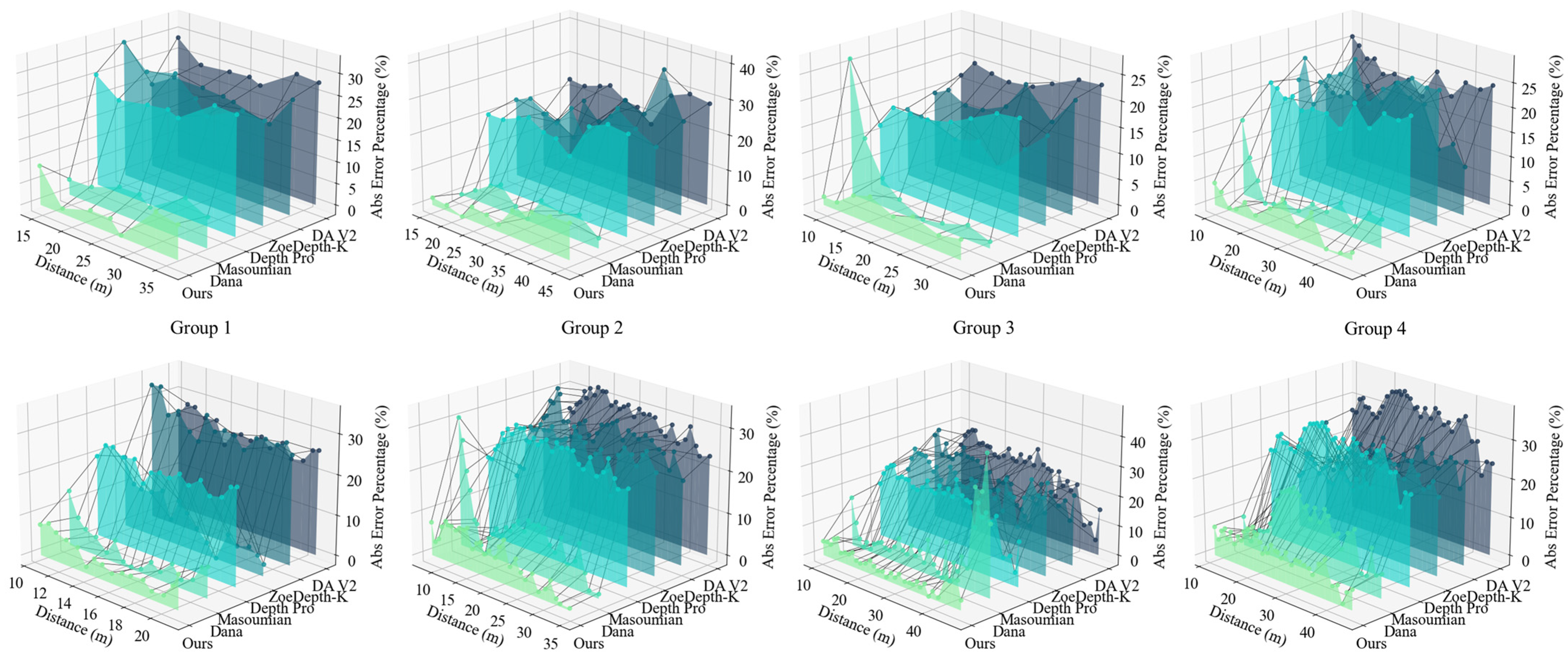
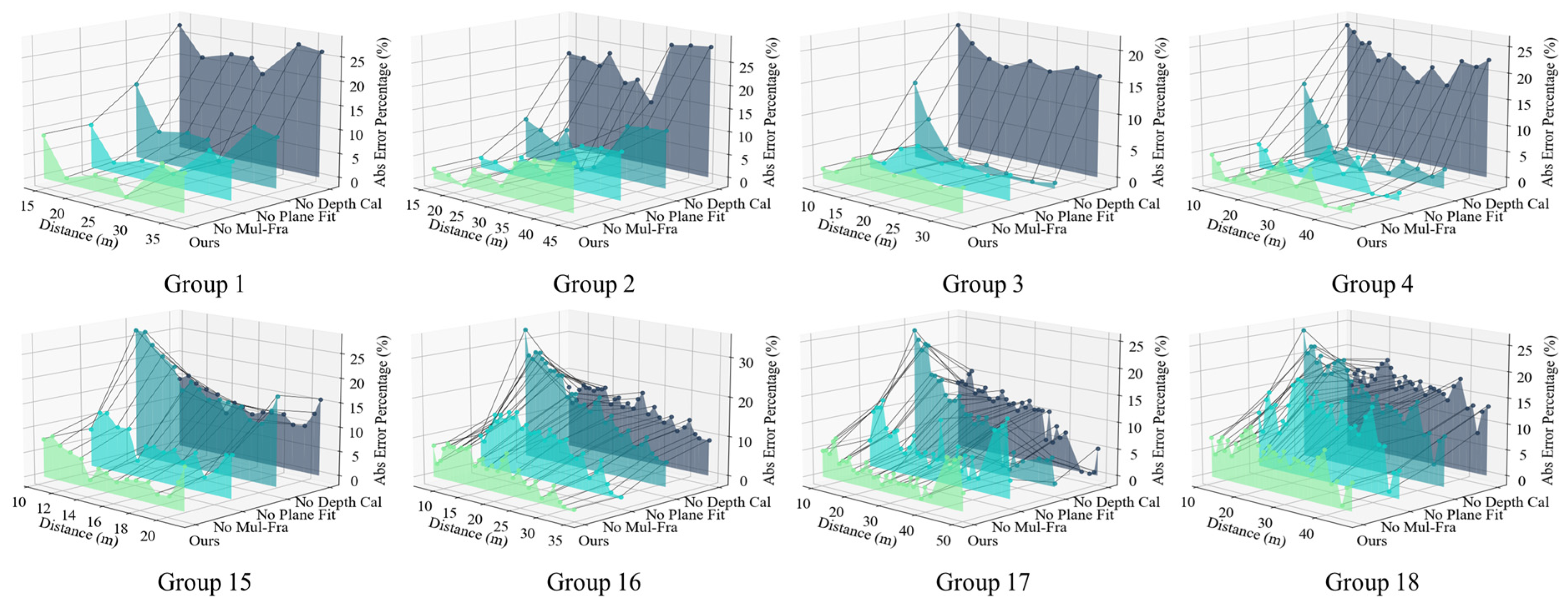
The metrics of δ < 1.25 , δ < 1.25 2 and δ < 1.25 3 are commonly used to evaluate the depth estimation accuracy and reliability. The proposed method achieves the δ < 1.25 of 0.972, demonstrating that it accurately estimates the depth under various real-world conditions. Under δ < 1.25 2 and δ < 1.25 3 conditions, the proposed method achieves an accuracy of 1.000, indicating that all predictions meet the required criteria under moderate and relaxed conditions. This also verifies the accuracy and reliability of the proposed method. This further confirms the robustness and reliability of the proposed method when evaluated across different levels of permissible error, ranging from strict accuracy requirements to relaxed thresholds. Figure 8 shows the error percentage trend of six metric depth estimation methods in 19 groups (G1–G19). The zoomed-in section further reveals the differences between our method and the Dana method. The Dana method exhibits significant prediction instability, manifested by severe fluctuations in error and large-scale deviations. From Figure 9, it can be observed that our method exhibits the lowest and most stable error surface at different distances and in different scenarios, further verifying the effectiveness of the proposed two-stage estimation strategy in improving robustness and generalization capability.
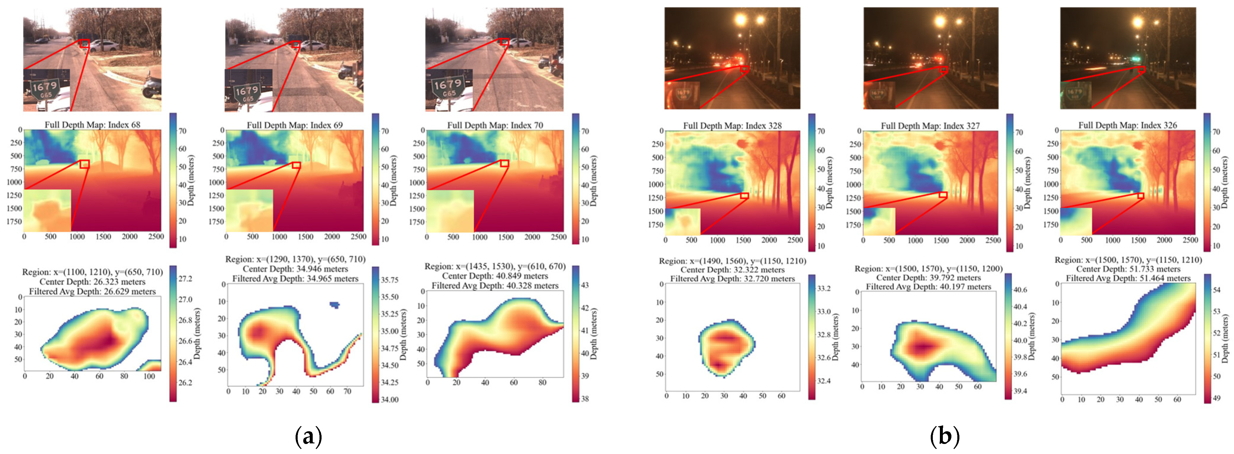
Figure 8 and Figure 9 present some failure cases from the proposed methods with high errors. Figure 10 presents two visual explanations of such failures. In Scene 1, the depth estimation is affected by interference from nearby vehicles, causing some target regions’ depth values to shift toward the depth range of adjacent vehicles. Although multi-frame weighted fusion can mitigate the impact of occluded areas on the final depth estimation, its optimization effect remains inferior to that of depth estimation scale recovery in non-interfered scenarios. In Scene 2, the overall frame contrast decreases in a low-light environment, making it difficult to distinguish the features of the distant milepost. This results in information loss in the target region affects the accuracy of depth estimation. In such cases, the effectiveness of weighted fusion significantly declines if successive multi-frame depth information exhibits large deviations or missing values. For Scene 1, temporal smoothing with longer multi-frame fusion and visibility-aware weighting could further alleviate the influence of occlusions from nearby vehicles. For Scene 2, applying low-light enhancement techniques such as gamma correction or exposure normalization can improve contrast and preserve target features under dark conditions.

4.3. Ablation Study

An ablation study is conducted to verify the contribution of the key modules in the proposed method, as shown in Table 2. “No Depth Cal” represents the removal of the scale recovery module based on a lower field-of-view road boundary. “No Plane Fit” indicates the removal of the road plane fitting method based on SVD and RANSAC optimization. “No Mul-Fra” corresponds to the removal of the multi-frame fusion optimization module. “Ours” refers to the full proposed method.
In Table 2, after removing the scale recovery module based on the lower field-of-view road boundary, the A b s   R e l increases from 0.055 to 0.216, nearly quadrupling the error; S q   R e l increases from 0.008 to 0.071, expanding by nearly nine times; R M S E increases from 3.421 to 7.351; and δ < 1.25 decreases from 0.972 to 0.463, while δ < 1.25 2 decreases from 1.000 to 0.662. The main reason is that the depth estimation entirely relies on the relative depth maps after removing the scale recovery module, leading to the low performance of converting relative depth values into metric ones. Furthermore, the absence of this module amplifies the impact of the camera field of view, scene geometry, and uneven target distribution, leading to increased depth estimation errors, especially in scenarios where depth estimation heavily depends on boundary points. The resulting error accumulation effect becomes more pronounced.
After removing the module of road plane fitting, the A b s   R e l increases from 0.055 to 0.102, S q   R e l increases from 0.008 to 0.018, R M S E increases from 3.421 to 3.622, and δ < 1.25 decreases from 0.972 to 0.875. This phenomenon derives from the fact that the module prevents an effective geometric model from being established for the road point set, leading to an increase in depth estimation directional errors. However, since the role of this module mainly focuses on optimizing the geometric relationship of the road plane, its overall impact on global error is relatively minor. Therefore, its influence on depth scale recovery is comparatively moderate.
After removing the module of the multi-frame fusion optimization, the R M S E increases from 3.421 to 4.224, while A b s   R e l , S q   R e l , and δ shows no significant changes. This is because, after removing this module, depth estimation relies entirely on single-frame information, leading to reduced robustness in complex scenarios (such as dynamic occlusions or illumination variations). Additionally, δ < 1.25 value drops significantly, while δ < 1.25 2 and δ < 1.25 3 , which represent more relaxed conditions, remain relatively stable. This indicates that extreme cases (e.g., occlusions) are relatively rare in the collected dataset, and single-frame estimation can still meet basic accuracy requirements in general scenarios. However, under extreme conditions such as occlusions and noise, multi-frame fusion optimization significantly reduces depth scale recovery errors, improving estimation accuracy and stability.
As shown in Figure 11 and Figure 12, removing the scale recovery module based on lower field-of-view road boundary tjs the error percentage, indicating that this module plays a key role in resolving scale ambiguity in monocular metric depth estimation and confirms it as a core component for ensuring the accuracy of depth recovery. The road plane fitting method based on SVD and RANSAC optimization enhances geometric consistency by filtering out noisy points and refining the overall structure. Due to the limited occlusion in the selected images, the multi-frame fusion module has a relatively limited impact on the overall error. it proves highly effective in more complex conditions involving dynamic occlusions or illumination changes, significantly improving robustness. Overall, the complete method outperforms variants that remove any submodule in all scenarios, further verifying the importance of collaborative work between modules. By leveraging the complementary advantages of each component, the proposed method achieves high-precision and highly robust metric depth estimation between the vehicle and the milepost.

4.4. Stability Study

(1) Distance segment performance evaluation study
To further evaluate the performance of the proposed method across different distance ranges, a distance-segmented error evaluation method is designed. Based on the true distance of the target, the data is divided into three segments: short-range (0–15 m), mid-range (15–30 m), and long-range (above 30 m). This allows for an analysis of the method’s adaptability and limitations under different distance conditions.
Table 3 presents the performance of the proposed method across different distance segments, where the mid-range segment exhibits the best performance. Except for R M S E , all other indicators outperform those in the short-range and long-range segments. This may be because, in the mid-range segment, the pixel size and depth estimation range are in an optimal balance, with less occlusion and noise interference, making depth estimation more likely to converge to the ground truth. In the short-range segment, although R M S E is better than in the mid-range segment; the other six indicators are slightly worse. This may be due to mileposts occupying a larger pixel proportion in close-range images, making depth estimation more sensitive to boundary pixels, which often carry higher noise and uncertainty, thus affecting overall performance. In the long-range segment, the method’s performance declines, likely due to the sparsity of target information, reduced resolution, and increased noise interference at the edges of the field of view, making depth estimation more challenging.
(2) Illumination condition performance evaluation study
To evaluate the performance of the proposed method under different illumination conditions, image datasets were selected from three typical lighting scenarios: strong illumination (daytime), normal illumination (dusk), and low illumination (nighttime). These datasets contain 166 frames, 118 frames, and 68 frames, respectively, allowing for an analysis of the method’s adaptability and limitations across different illumination conditions.
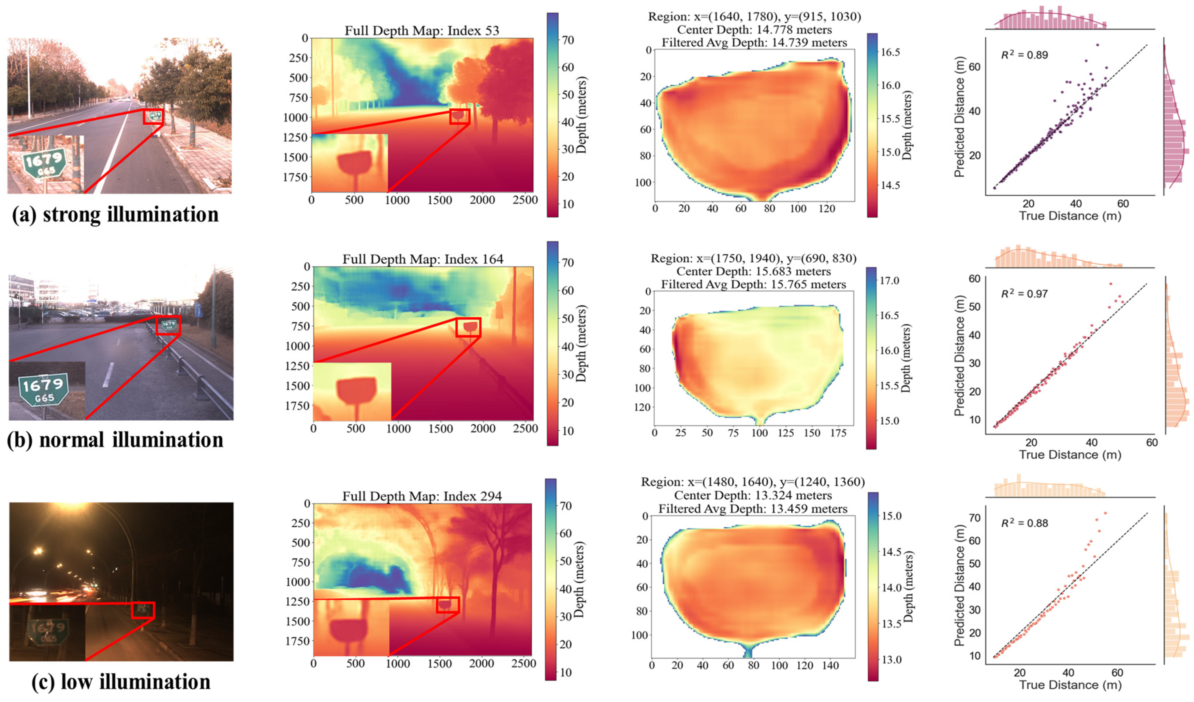
Table 4 presents the performance of the proposed method under different illumination conditions. Under normal illumination at dusk, the method achieves the highest accuracy and the lowest error. This may be because the moderate lighting and high image quality ensure that the milepost features remain clear and well-defined, improving depth scale recovery accuracy. In Figure 13, under strong illumination conditions, the performance of the proposed method slightly declines, possibly due to surface reflections on the milepost or the presence of shadows caused by strong sunlight, leading to overexposure or uneven brightness in certain areas, which affects depth scale recovery accuracy. However, even in this scenario, the method achieves an A b s   R e l of 0.052 and a R M S E of 3.891, indicating that despite the reflection effects, the proposed method maintains high accuracy. Under low-light nighttime conditions, the A b s   R e l increases to 0.082, and the R M S E rises to 4.368, indicating a further decline in performance. This may be due to insufficient illumination, which degrades image quality and reduces the visibility of target features, thereby affecting the stability of the algorithm. The last column of Figure 13 shows the images under three illumination conditions (strong, normal, and low illumination), along with the regression fit between the predicted distance and the actual distance, and visualized analysis using edge distribution histograms. The results showed that under normal illumination conditions, the fitting accuracy was the highest, with an R2 of 0.97; Under strong and weak light conditions, R2 is 0.89 and 0.88, respectively, although slightly decreased, it still maintains a high estimation accuracy. This result indicates that normal illumination is beneficial for the accuracy of depth estimation, while different illumination conditions can have an impact on estimation performance, especially in situations where strong illumination or low illumination imaging is unclear. However, the proposed method still exhibits good robustness and reliability in illumination scenarios.
(3) Road condition performance evaluation study
To evaluate the adaptability and robustness of the proposed method under different road conditions, experiments were conducted on two typical road types: flat roads and curved roads. This analysis aims to investigate the impact of road geometry characteristics on the performance of the proposed method.
Table 5 presents the performance results of the proposed method under different road conditions. In flat road scenarios, metrics such as A b s   R e l and R M S E show outstanding performance, with errors distributed more compactly and estimation results closer to the ground truth. In curved road scenarios, error metrics show a slight increase, which may be due to the simpler geometric characteristics of flat roads, where lane lines and target object edges are more stable, providing sufficient geometric and texture features for depth estimation scale recovery. In contrast, the complex geometric structure and dynamic perspective changes in curved road scenarios introduce depth uncertainty and viewpoint distortion, leading to increased estimation errors. However, despite these challenges, the overall performance remains satisfactory, demonstrating high accuracy and robustness in depth estimation scale recovery.

5. Conclusions

This paper has proposed a two-stage monocular metric depth estimation with boundary calibration and geometric optimization, aiming to address the unreliable and inaccurate estimation problem due to the camera installation angle, the milepost inclination, and occlusions. An experiment using 352 samples with real images and depth measurement demonstrates the effectiveness of the proposed method. The following conclusions can be drawn.
(1) The proposed method outperforms other state-of-the-art approaches in monocular metric depth estimation, achieving an absolute relative error of 0.055 and a threshold accuracy of 0.972, demonstrating its effectiveness in providing a reliable and accurate depth estimation solution across various real-world conditions.
(2) The improvement of the proposed method is attributed to depth calibration using field-of-view boundary road points and multi-frame fusion optimization. Scale recovery module effectively eliminates scale ambiguity, reducing the Abs Rel error from 0.216 to 0.055. Road-plane-based geometric optimization addresses depth estimation inaccuracies resulting from non-parallel camera installation and milepost inclination, while multi-frame fusion enhances robustness by mitigating the effects of occlusions and camera perspective limitations, improving RMSE from 4.224 to 3.421.
(3) The proposed method exhibits high stability in monocular metric depth estimation, maintaining consistent accuracy across varying environments, including different distances, illuminations, and road conditions. For example, it achieves Abs Rel = 0.082 under low illumination. Across distances, performance is nearly perfect at short range (δ < 1.25 = 1.000) and still reliable at long range (Abs Rel = 0.079). With high accuracy under loose error tolerance levels, it demonstrates robustness and reliability, ensuring stable depth estimation in real-world applications.
(4) The future work should focus on two aspects. First, the proposed method should incorporate dynamic object tracking and occlusion compensation strategies to further improve the robustness of the proposed method on dynamic occlusion scenarios. Second, future studies should integrate high-resolution sensors and multi-modal data fusion strategies to supplement geometric and spatial information for long-distance targets.

Author Contributions

Conceptualization, T.M. and Z.T.; methodology, E.Z., T.M. and Z.T.; software, E.Z. and H.Y.; validation, E.Z., J.L. and Z.X.; formal analysis, E.Z. and Z.T.; investigation, E.Z., J.L. and Z.X.; resources, T.M. and Z.T.; data curation, E.Z., J.L. and Z.X.; writing—original draft preparation, E.Z.; writing—review and editing, T.M. and Z.T.; visualization, E.Z.; supervision, T.M. and Z.T.; funding acquisition, T.M. and Z.T. All authors have read and agreed to the published version of the manuscript.

Funding

This research was also funded by the National Natural Science Foundation of China under Grant 52308447, the Jiangsu Province Youth Science and Technology Talent Lifting Project under Grant JSTJ-2024-089, and the Xinjiang Uygur Autonomous Region Key Research and Development Project, grant number 2021B01005.

Data Availability Statement

Code and data will be made available on request.

Conflicts of Interest

The authors declare no conflicts of interest.

References

  1. Gong, Y.; Zhang, X.; Feng, J.; He, X.; Zhang, D. LiDAR-Based HD Map Localization Using Semantic Generalized ICP with Road Marking Detection. In Proceedings of the 2024 IEEE/RSJ International Conference on Intelligent Robots and Systems (IROS), Abu Dhabi, United Arab Emirates, 14 October 2024; pp. 3379–3386. [Google Scholar]
  2. Cong, L.; Li, D.; Meng, K.; Zhu, S. Road-Aware Localization With Salient Feature Matching in Heterogeneous Networks. In Proceedings of the 2024 IEEE Wireless Communications and Networking Conference (WCNC), Dubai, United Arab Emirates, 21 April 2024; pp. 1–6. [Google Scholar]
  3. Nemec, D.; Šimák, V.; Janota, A.; Hruboš, M.; Bubeníková, E. Precise Localization of the Mobile Wheeled Robot Using Sensor Fusion of Odometry, Visual Artificial Landmarks and Inertial Sensors. Robot. Auton. Syst. 2019, 112, 168–177. [Google Scholar] [CrossRef]
  4. Wan, G.; Yang, X.; Cai, R.; Li, H.; Zhou, Y.; Wang, H.; Song, S. Robust and Precise Vehicle Localization Based on Multi-Sensor Fusion in Diverse City Scenes. In Proceedings of the 2018 IEEE International Conference on Robotics and Automation (ICRA), Brisbane, QLD, Australia, 21–25 May 2018; pp. 4670–4677. [Google Scholar]
  5. Zhang, H.; Chen, C.-C.; Vallery, H.; Barfoot, T.D. GNSS/Multisensor Fusion Using Continuous-Time Factor Graph Optimization for Robust Localization. IEEE Trans. Robot. 2024, 40, 4003–4023. [Google Scholar] [CrossRef]
  6. Liu, H.; Ma, R. Research on Automatic Mileage Pile Positioning Technology Based on Multi-Sensor Fusion. 2023. Available online: https://ssrn.com/abstract=4598722 (accessed on 20 July 2025).
  7. Liu, H.; Ma, R. An Efficient and Automatic Method Based on Monocular Camera and GNSS for Collecting and Updating Geographical Coordinates of Mileage Pile in Highway Digital Twin Map. Meas. Sci. Technol. 2024, 35, 126011. [Google Scholar] [CrossRef]
  8. Eigen, D.; Puhrsch, C.; Fergus, R. Depth Map Prediction from a Single Image Using a Multi-Scale Deep Network. In Advances in Neural Information Processing Systems, Proceedings of the 28th International Conference on Neural Information Processing Systems Montreal, QC, Canada, 8–13 December 2014; MIT Press: Cambridge, MA, USA, 2014; Volume 27. [Google Scholar]
  9. Zhang, G.; Tang, X.; Wang, L.; Cui, H.; Fei, T.; Tang, H.; Jiang, S. Repmono: A Lightweight Self-Supervised Monocular Depth Estimation Architecture for High-Speed Inference. Complex Intell. Syst. 2024, 10, 7927–7941. [Google Scholar] [CrossRef]
  10. Xi, Y.; Li, S.; Xu, Z.; Zhou, F.; Tian, J. LapUNet: A Novel Approach to Monocular Depth Estimation Using Dynamic Laplacian Residual U-Shape Networks. Sci. Rep. 2024, 14, 23544. [Google Scholar] [CrossRef]
  11. Sui, X.; Gao, S.; Xu, A.; Zhang, C.; Wang, C.; Shi, Z. Lightweight Monocular Depth Estimation Using a Fusion-Improved Transformer. Sci. Rep. 2024, 14, 22472. [Google Scholar] [CrossRef]
  12. Cheng, J.; Liu, L.; Xu, G.; Wang, X.; Zhang, Z.; Deng, Y.; Zang, J.; Chen, Y.; Cai, Z.; Yang, X. Monster: Marry Monodepth to Stereo Unleashes Power. In Proceedings of the IEEE/CVF Conference on Computer Vision and Pattern Recognition (CVPR), Nashville, TN, USA, 9–14 June 2025; pp. 6273–6282. [Google Scholar]
  13. Song, Z.; Wang, Z.; Li, B.; Zhang, H.; Zhu, R.; Liu, L.; Jiang, P.; Zhang, T. DepthMaster: Taming Diffusion Models for Monocular Depth Estimation. arXiv 2025, arXiv:2501.02576. [Google Scholar] [CrossRef]
  14. Kuznietsov, Y.; Stuckler, J.; Leibe, B. Semi-Supervised Deep Learning for Monocular Depth Map Prediction. In Proceedings of the IEEE Conference on Computer Vision and Pattern Recognition (CVPR), Honolulu, HI, USA, 21–26 July 2017; pp. 6647–6655. [Google Scholar]
  15. Zama Ramirez, P.; Poggi, M.; Tosi, F.; Mattoccia, S. Geometry Meets Semantics for Semi-Supervised Monocular Depth Estimation. In Computer Vision—ACCV 2018, Proceedings of the Asian Conference on Computer Vision (ACCV), Perth, Australia, 2–6 December 2018; Springer International Publishing: Cham, Switzerland, 2018; pp. 298–313. [Google Scholar]
  16. Rahman, M.A.; Fattah, S.A. Semi-Supervised Semantic Depth Estimation Using Symbiotic Transformer and NearFarMix Augmentation. In Proceedings of the IEEE/CVF Winter Conference on Applications of Computer Vision (WACV), Waikoloa, HI, USA, 3–7 January 2024; IEEE: Piscataway, NJ, USA, 2024; pp. 250–259. [Google Scholar]
  17. Song, K.; Yoon, K.J. Learning Monocular Depth Estimation via Selective Distillation of Stereo Knowledge. arXiv 2022, arXiv:2205.08668. [Google Scholar] [CrossRef]
  18. Gurram, A.; Urfalioglu, O.; Halfaoui, I.; Bouzaraa, F.; Lopez, A.M. Semantic monocular depth estimation based on artificial intelligence. IEEE Intell. Transp. Syst. Mag. 2020, 13, 99–103. [Google Scholar] [CrossRef]
  19. Garg, R.; Bg, V.K.; Carneiro, G.; Reid, I. Unsupervised CNN for Single View Depth Estimation: Geometry to the Rescue. In Computer Vision—ECCV 2016; Leibe, B., Matas, J., Sebe, N., Welling, M., Eds.; Lecture Notes in Computer Science; Springer: Cham, Switzerland, 2016; pp. 740–756. [Google Scholar]
  20. Zhou, T.; Brown, M.; Snavely, N.; Lowe, D.G. Unsupervised learning of depth and ego-motion from video. In Proceedings of the IEEE Conference on Computer Vision and Pattern Recognition, Honolulu, HI, USA, 21–26 July 2017. [Google Scholar]
  21. Shim, D.; Kim, H.J. SwinDepth: Unsupervised Depth Estimation Using Monocular Sequences via Swin Transformer and Densely Cascaded Network. In Proceedings of the 2023 IEEE International Conference on Robotics and Automation (ICRA), London, UK, 29 May 2023; pp. 4983–4990. [Google Scholar]
  22. Lian, L.; Qin, Y.; Cao, Z.; Gao, Y.; Bai, J.; Ge, X.; Guo, B. A Continuous Autonomous Train Positioning Method Using Stereo Vision and Object Tracking. IEEE Intell. Transp. Syst. Mag. 2024, 16, 6–62. [Google Scholar] [CrossRef]
  23. Hui, T.-W. RM-Depth: Unsupervised Learning of Recurrent Monocular Depth in Dynamic Scenes. In Proceedings of the 2022 IEEE/CVF Conference on Computer Vision and Pattern Recognition (CVPR), New Orleans, LA, USA, 18–24 June 2022; pp. 1665–1674. [Google Scholar]
  24. Chawla, H.; Varma, A.; Arani, E.; Wang, J. Continual Learning of Unsupervised Monocular Depth from Videos. In Proceedings of the 2024 IEEE/CVF Winter Conference on Applications of Computer Vision (WACV), Waikoloa, HI, USA, 3–8 January 2024; pp. 8419–8429. [Google Scholar]
  25. Saunders, K.; Vogiatzis, G.; Manso, L.J. Self-Supervised Monocular Depth Estimation: Let’s Talk about the Weather. In Proceedings of the IEEE/CVF International Conference on Computer Vision (ICCV), Paris, France, 2–3 October 2023; pp. 11255–11265. [Google Scholar]
  26. Fu, H.; Gong, M.; Wang, C.; Batmanghelich, K.; Tao, D. Deep Ordinal Regression Network for Monocular Depth Estimation. In Proceedings of the 2018 IEEE/CVF Conference on Computer Vision and Pattern Recognition, Salt Lake City, UT, USA, 18–23 June 2018; pp. 2002–2011. [Google Scholar]
  27. Guizilini, V.; Vasiljevic, I.; Chen, D.; Ambruş, R.; Gaidon, A. Towards Zero-Shot Scale-Aware Monocular Depth Estimation. In Proceedings of the 2023 IEEE/CVF International Conference on Computer Vision (ICCV), Paris, France, 2–3 October 2023; pp. 9233–9243. [Google Scholar]
  28. Bhat, S.F.; Birkl, R.; Wofk, D.; Wonka, P.; Esteves, C. ZoeDepth: Zero-Shot Transfer by Combining Relative and Metric Depth. arXiv 2023, arXiv:2302.12288. [Google Scholar]
  29. Bochkovskii, A.; Delaunoy, A.; Germain, H.; Georgoulis, S.; Proesmans, M.; Van Gool, L. Depth Pro: Sharp Monocular Metric Depth in Less than a Second. arXiv 2024, arXiv:2410.02073. [Google Scholar] [CrossRef]
  30. Piccinelli, L.; Yang, Y.H.; Sakaridis, C.; Van Gool, L. UniDepth: Universal Monocular Metric Depth Estimation. In Proceedings of the IEEE/CVF Conference on Computer Vision and Pattern Recognition (CVPR), Seattle, WA, USA, 17–21 June 2024; pp. 10106–10116. [Google Scholar]
  31. Yang, L.; Kang, B.; Huang, Z.; Chen, S.; Wang, S.; Zhao, H.; Feng, J. Depth Anything: Unleashing the Power of Large-Scale Unlabeled Data. In Proceedings of the IEEE/CVF Conference on Computer Vision and Pattern Recognition (CVPR), Seattle, WA, USA, 17–21 June 2024; pp. 10371–10381. [Google Scholar]
  32. Chawla, H.; Varma, A.; Arani, E.; Zonooz, B. Multimodal Scale Consistency and Awareness for Monocular Self-Supervised Depth Estimation. In Proceedings of the 2021 IEEE International Conference on Robotics and Automation (ICRA), Xi’an, China, 30 May 2021; pp. 5140–5146. [Google Scholar]
  33. Zhang, S.; Zhang, J.; Tao, D. Towards Scale-Aware, Robust, and Generalizable Unsupervised Monocular Depth Estimation by Integrating IMU Motion Dynamics. In Computer Vision—ECCV 2022, Proceedings of the 17th European Conference, Tel Aviv, Israel, 23–27 October 2022; European Conference on Computer Vision; Springer Nature Switzerland: Cham, Switzerland, 2022; pp. 143–160. [Google Scholar]
  34. Hu, M.; Yin, W.; Zhang, C.; Cai, Z.; Long, X.; Chen, H.; Wang, K.; Yu, G.; Shen, C.; Shen, S. Metric3D v2: A Versatile Monocular Geometric Foundation Model for Zero-Shot Metric Depth and Surface Normal Estimation. IEEE Trans. Pattern Anal. Mach. Intell. 2024, 46, 10579–10596. [Google Scholar] [CrossRef] [PubMed]
  35. Lin, H.; Peng, S.; Chen, J.; Peng, S.; Sun, J.; Liu, M.; Bao, H.; Feng, J.; Zhou, X.; Kang, B. Prompting Depth Anything for 4K Resolution Accurate Metric Depth Estimation. In Proceedings of the Computer Vision and Pattern Recognition Conference, Nashville, TN, USA, 11–15 June 2025; pp. 17070–17080. [Google Scholar]
  36. Cui, X.-Z.; Feng, Q.; Wang, S.-Z.; Zhang, J.-H. Monocular Depth Estimation with Self-Supervised Learning for Vineyard Unmanned Agricultural Vehicle. Sensors 2022, 22, 721. [Google Scholar] [CrossRef]
  37. Gelso, E.R.; Sjoberg, J. Consistent Threat Assessment in Rear-End Near-Crashes Using BTN and TTB Metrics, Road Information and Naturalistic Traffic Data. IEEE Intell. Transp. Syst. Mag. 2017, 9, 74–89. [Google Scholar] [CrossRef]
  38. Elazab, G.; Gräber, T.; Unterreiner, M.; Hellwich, O. MonoPP: Metric-Scaled Self-Supervised Monocular Depth Estimation by Planar-Parallax Geometry in Automotive Applications. In Proceedings of the 2025 IEEE/CVF Winter Conference on Applications of Computer Vision (WACV), Tucson, AZ, USA, 26 February 2025; pp. 2777–2787. [Google Scholar]
  39. Zheng, C.; Cham, T.J.; Cai, J. T2net: Synthetic-to-Realistic Translation for Solving Single-Image Depth Estimation Tasks. In Proceedings of the European Conference on Computer Vision (ECCV), Munich, Germany, 8–14 September 2018; pp. 767–783. [Google Scholar]
  40. Lo, S.-Y.; Wang, W.; Thomas, J.; Zheng, J.; Patel, V.M.; Kuo, C.-H. Learning Feature Decomposition for Domain Adaptive Monocular Depth Estimation. In Proceedings of the 2022 IEEE/RSJ International Conference on Intelligent Robots and Systems (IROS), Kyoto, Japan, 23 October 2022; pp. 8376–8382. [Google Scholar]
  41. Li, Z.; Bhat, S.F.; Wonka, P. PatchRefiner: Leveraging Synthetic Data for Real-Domain High-Resolution Monocular Metric Depth Estimation. In Computer Vision—ECCV 2024, Proceedings of the European Conference on Computer Vision (ECCV), Cham, Switzerland, 29 September–4 October 2024; Springer Nature Switzerland: Cham, Switzerland, 2024; pp. 250–267. [Google Scholar]
  42. Zhang, C.; Weng, X.; Cao, Y.; Zhang, M.; Wang, L.; Li, H. Monocular Absolute Depth Estimation from Motion for Small Unmanned Aerial Vehicles by Geometry-Based Scale Recovery. Sensors 2024, 24, 4541. [Google Scholar] [CrossRef]
  43. Masoumian, A.; Marei, D.G.F.; Abdulwahab, S.; Abualkishik, A.Z. Absolute Distance Prediction Based on Deep Learning Object Detection and Monocular Depth Estimation Models. In Artificial Intelligence Research and Development; IOS Press: Amsterdam, The Netherlands, 2021; pp. 325–334. [Google Scholar]
  44. Dana, A.; Carmel, N.; Shomer, A.; Zvirin, Y.; Bagon, S.; Dekel, T. Do More with What You Have: Transferring Depth-Scale from Labeled to Unlabeled Domains. In Proceedings of the IEEE/CVF Conference on Computer Vision and Pattern Recognition, Piscataway, NJ, USA, 16–22 June 2024; pp. 4440–4450. [Google Scholar]
  45. Zhu, R.; Wang, C.; Song, Z.; Zhang, H.; Sun, J. ScaleDepth: Decomposing Metric Depth Estimation into Scale Prediction and Relative Depth Estimation. arXiv 2024, arXiv:2407.08187. [Google Scholar] [CrossRef]
  46. McCraith, R.; Neumann, L.; Vedaldi, A. Calibrating Self-Supervised Monocular Depth Estimation. arXiv 2020, arXiv:2009.07714. [Google Scholar]
  47. Xue, F.; Zhuo, G.; Huang, Z.; Fu, W.; Wu, Z.; Ang, M.H. Toward Hierarchical Self-Supervised Monocular Absolute Depth Estimation for Autonomous Driving Applications. In Proceedings of the 2020 IEEE/RSJ International Conference on Intelligent Robots and Systems (IROS), Las Vegas, NV, USA, 24 October 2020; pp. 2330–2337. [Google Scholar]
  48. Yang, W.; Li, H.; Li, X.; Wang, Z.; Zhang, B. UAV Image Target Localization Method Based on Outlier Filter and Frame Buffer. Chin. J. Aeronaut. 2024, 37, 375–390. [Google Scholar] [CrossRef]
  49. Khanam, R.; Hussain, M. Yolov11: An Overview of the Key Architectural Enhancements. arXiv 2024, arXiv:2410.17725. [Google Scholar] [CrossRef]
  50. Yang, L.; Kang, B.; Huang, Z.; Zhao, Z.; Xu, X.; Feng, J.; Zhao, H. Depth Anything v2. Adv. Neural Inf. Process. Syst. 2024, 37, 21875–21911. [Google Scholar]
  51. National Standard GB 5768.2-2022; Road Traffic Signs and Markings—Part 2: Road Traffic Signs. Standardization Administration of China: Beijing, China, 2022.
Figure 1. Workflow of the milepost-assisted vehicle positioning method. The process consists of four main steps: (1) Onboard image acquisition using a forward-facing camera; (2) Milepost detection and recognition via object detection and OCR; (3) Location extraction by converting image coordinates to road coordinates; and (4) GPS integration for accurate positioning. The lower illustration shows the distance deviation caused by the non-parallel alignment between the camera and the milepost.
Electronics 14 03446 g001
Figure 2. Overall framework of the proposed two-stage monocular metric depth estimation method. Stage 1 performs the transformation from relative depth to initial metric depth, while Stage 2 refines the initial metric depth estimation through geometric optimization.
Electronics 14 03446 g002
Figure 3. Scale recovery based on field-of-view lower boundary road points. The green shaded area represents the FoV, the red solid line indicates the closest boundary of the FoV, and the green solid line represents the farthest boundary. The red dashed line marks the distance from the points entering the FoV to the vehicle, and the green dashed arrow denotes the distance between milepost and vehicle.
Electronics 14 03446 g003
Figure 4. Depth estimation network structure. The input image is divided into patches and processed through position embedding, linear projection, and multiple transformer layers. Features are reassembled and fused to refine depth prediction, with the final relative depth map generated by the head module.
Electronics 14 03446 g004
Figure 5. Effects of camera installation angle and milepost inclination on depth estimation. (a) The installation angle changes the perceived position of the milepost, potentially causing depth errors. (b) A tilted milepost alters its geometric projection in the image, impacting depth estimation.
Electronics 14 03446 g005
Figure 6. Pipeline of the Road Plane Fitting Method Based on SVD and RANSAC Optimization input data projection into 3D points, preprocessing and filtering, plane hypothesis with RANSAC, best plane selection, refinement using SVD, pose alignment, and depth estimation between vehicle and milepost.
Electronics 14 03446 g006
Figure 7. Illustration of data collection. A camera mounted on the vehicle to capture road images, acquisition software for data recording, and a laser rangefinder for ground-truth distance measurement. Milepost serves as a reference point.
Electronics 14 03446 g007
Figure 8. Result of the comparison study. The performance of different methods is evaluated using the error percentage. The images are grouped by scenario and sorted by increasing distance in each group. A zoomed-in section highlights the performance differences between Dana and the proposed method.
Electronics 14 03446 g008
Figure 9. Three-dimensional wall chart of absolute error percentage across selected groups and methods, highlighting performance differences under different methods and scenarios.
Electronics 14 03446 g009
Figure 10. Analysis of depth scale recovery results in high-error scenes: (a) daytime and (b) nighttime. Each row shows input images, depth maps, and depth of mileposts, highlighting milepost regions with high errors due to illumination, occlusion or other factors.
Electronics 14 03446 g010
Figure 11. The result of ablation study. The figure compares the impact of different components on depth estimation accuracy. The error percentage is used to evaluate different configurations.
Electronics 14 03446 g011
Figure 12. The 3D wall chart of absolute error percentage across selected groups and methods. The figure highlights performance differences under different methods and scenarios.
Electronics 14 03446 g012
Figure 13. Comparison of effects under different illumination conditions at a similar distance. The comparison includes (a) strong illumination, (b) normal illumination, (c) low illumination. These three scenarios are compared at similar distances and present different depth estimation results. The last column shows regression plots with marginal histograms between predicted and true distances under different illumination conditions.
Electronics 14 03446 g013
Table 1. Results of the comparison study.
MethodLower Is Better ↓Higher Is Better ↑
A b s   R e l S q   R e l R M S E R M S E   l o g Latency δ < 1.25 δ < 1.25 2 δ < 1.25 3 FPS
DA V2 [50]0.2120.0505.9620.257360.4491.0001.00028
ZoeDepth-K [28]0.2160.0717.3510.330450.4630.6621.00022
Depth Pro [29]0.2380.0678.0460.318500.3440.8750.98620
Masoumian [43]0.1290.0428.5700.167590.8810.9600.99717
Dana [44]0.1950.0425.6840.234420.5341.0001.00024
Ours0.0550.0083.4210.080300.9721.0001.00033
Bold numbers indicate the best performance, and underlined numbers represent the second-best performance.
Table 2. Results of the ablation study.
MethodLower Is Better ↓Higher Is Better ↑
A b s   R e l S q   R e l R M S E R M S E   l o g δ < 1.25 δ < 1.25 2 δ < 1.25 3
No Depth Cal0.2160.0717.3510.3300.4630.6621.000
No Plane Fit0.1020.0183.6220.1390.8751.0001.000
No Mul-Fra0.0810.0134.2240.1080.9601.0001.000
Ours0.0550.0083.4210.0800.9721.0001.000
Bold numbers indicate the best performance, and underlined numbers represent the second-best performance.
Table 3. Performance evaluation of the method across different distance segments.
MethodLower Is Better ↓Higher Is Better ↑
A b s   R e l S q   R e l R M S E R M S E   l o g δ < 1.25 δ < 1.25 2 δ < 1.25 3
short-range0.0460.0030.6670.0581.0001.0001.000
mid-range0.0380.0021.0700.0491.0001.0001.000
long-range0.0790.0175.4890.1130.9231.0001.000
Bold numbers indicate the best performance, and underlined numbers represent the second-best performance.
Table 4. Performance evaluation of the method under different illumination conditions.
MethodLower Is Better ↓Higher Is Better ↑
A b s   R e l S q   R e l R M S E R M S E   l o g δ < 1.25 δ < 1.25 2 δ < 1.25 3
Strong0.0520.0103.8910.0870.9581.0001.000
Normal0.0440.0031.6180.0550.9921.0001.000
Low0.0820.0104.3680.0970.9711.0001.000
Bold numbers indicate the best performance, and underlined numbers represent the second-best performance.
Table 5. Performance evaluation of the method across different road conditions.
MethodLower Is Better ↓Higher Is Better ↑
A b s   R e l S q   R e l R M S E R M S E   l o g δ < 1.25 δ < 1.25 2 δ < 1.25 3
Flat road0.0530.0083.2770.0800.9701.0001.000
Curved road0.0620.0083.8270.0820.9571.0001.000
Bold numbers indicate the best performance.
Disclaimer/Publisher’s Note: The statements, opinions and data contained in all publications are solely those of the individual author(s) and contributor(s) and not of MDPI and/or the editor(s). MDPI and/or the editor(s) disclaim responsibility for any injury to people or property resulting from any ideas, methods, instructions or products referred to in the content.