Fine-Grained Fault Sensitivity Analysis of Vision Transformers Under Soft Errors

Abstract

Over the past decade, deep neural networks (DNNs) have revolutionized the fields of computer vision (CV) and natural language processing (NLP), achieving unprecedented performance across a variety of tasks. The Vision Transformer (ViT) has emerged as a powerful alternative to convolutional neural networks (CNNs), leveraging self-attention mechanisms to capture long-range dependencies and global context. Owing to their flexible architecture and scalability, ViTs have been widely adopted in safety-critical applications such as autonomous driving, where system reliability is paramount. However, ViTs’ reliability issues induced by soft errors in large-scale digital integrated circuits have generally been overlooked. In this paper, we present a fine-grained fault sensitivity analysis of ViT variants under bit-flip fault injections, focusing on different ViT models, transformer encoder layers, weight matrix types, and attention-head dimensions. Experimental results demonstrate that the first transformer encoder layer is susceptible to soft errors due to its essential role in local and global feature extraction. Moreover, in the middle and later layers, the Multi-Layer Perceptron (MLP) sub-blocks dominate the computational workload and significantly influence representation learning, making them critical points of vulnerability. These insights highlight key reliability bottlenecks in ViT architectures when deployed in error-prone environments.

1. Introduction

During the past few decades, deep neural networks (DNNs) have achieved significant advancements in the fields of computer vision (CV) [1,2,3,4] and natural language processing (NLP) [5,6,7,8]. The attention-based transformer network proposed in 2017 [9] addressed the limitations of sequential computation in recurrent neural networks (RNNs) [10] and long short-term memory (LSTM) networks [11]. This novel architecture has been successfully applied to image classification and object detection, such as Vision Transformer (ViT) [12] and Detection Transformer (DETR) [13]. Due to their large number of parameters and self-attention mechanism, ViTs can be pre-trained on large-scale datasets for fundamental tasks and subsequently fine-tuned to small datasets for specific tasks while maintaining high accuracy [14].

Despite extensive research on optimizing ViTs for performance and accuracy [15,16,17], issues related to their dependability or reliability remain largely under-explored. When ViTs are deployed in safety-critical applications such as autonomous driving, they face two key reliability challenges: (1) Due to their large number of parameters, ViTs often suffer from high computational complexity [18] and an increased susceptibility to hardware-induced errors [19]. (2) With continuous progress in integrated circuit technologies, the probability of soft error rises steadily in Very Large-Scale Integration (VLSI) [20,21].

The reliability of convolutional neural networks (CNNs) has been extensively researched, ranging from architecture-level sensitivity [22], data-type implementation [23], and model compression strategies [24], to hardware-level resilience designs [25,26]. Recent works on ViT robustness have primarily focused on adversarial defense [27], privacy preservation [28,29], and quantization/pruning techniques [30,31]. However, studies specifically targeting the fault resilience of ViTs under hardware errors are still in their infancy, with existing works limited to basic simulation and lacking fine-grained analysis [32,33]. To bridge this gap, we performed a systematic and fine-grained fault sensitivity analysis on quantized ViT models under realistic deployment conditions.

The following summarizes our main contributions:

• We proposed a fault resilience evaluation framework tailored to ViTs, incorporating realistic deployment settings via Int8 quantization.
• We performed a fine-grained fault sensitivity analysis across four key dimensions—model-wise, layer-wise, type-wise, and head-wise—under bit-flip fault injection scenarios.
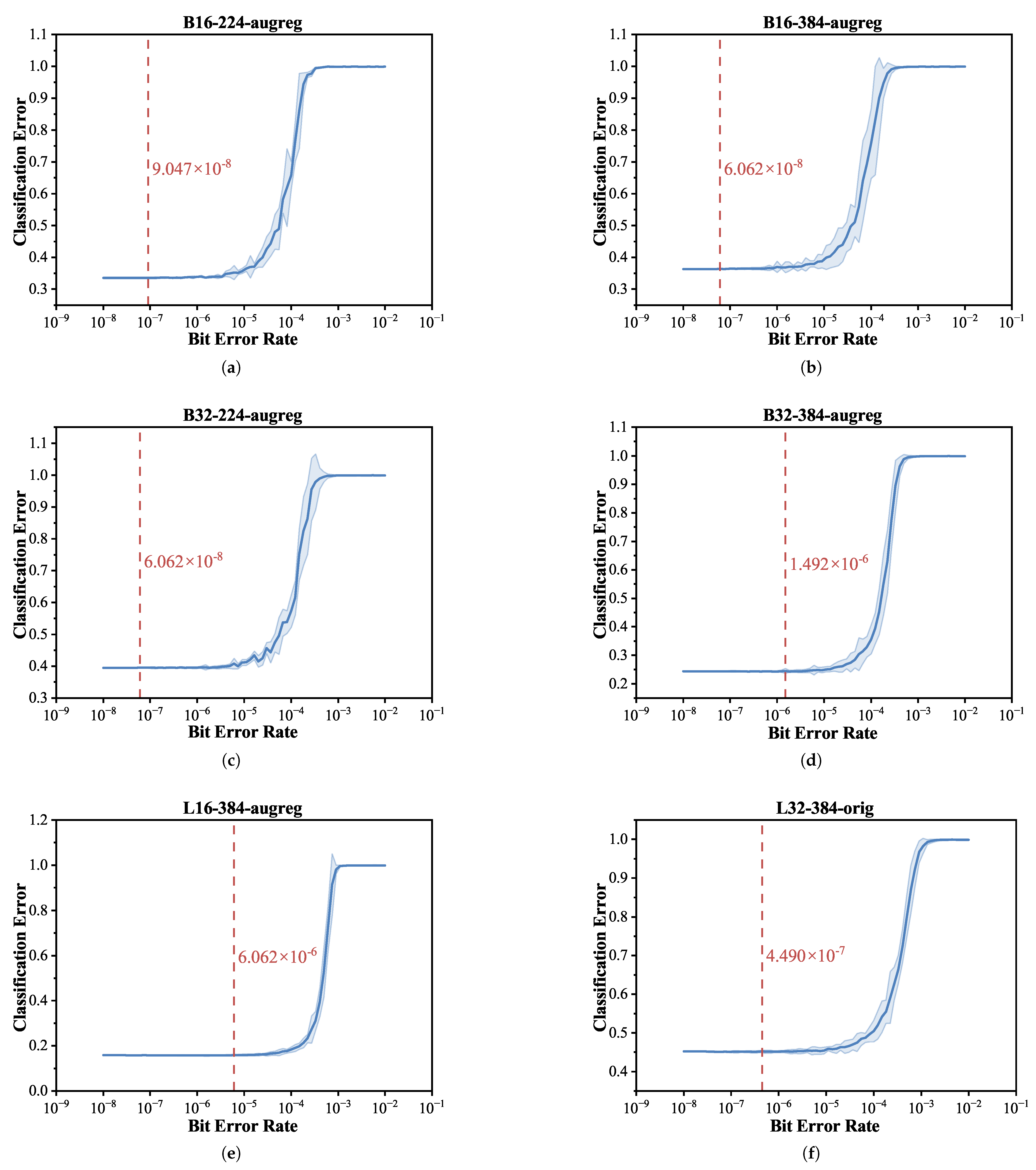
• From a model-wise perspective, we observed that architectural parameters such as model size and patch size substantially influence error resilience, with BER thresholds varying by several orders of magnitude across models.
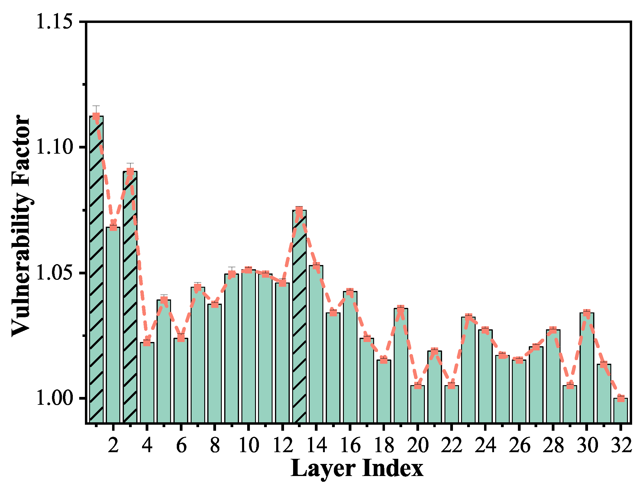
• At the layer-wise level, we identified the first transformer encoder layer as particularly susceptible to soft errors, owing to its foundational role in hierarchical feature extraction. Middle and later layers’ MLP sub-blocks also emerge as critical vulnerability points due to their dominant computational load and contribution to representation learning.
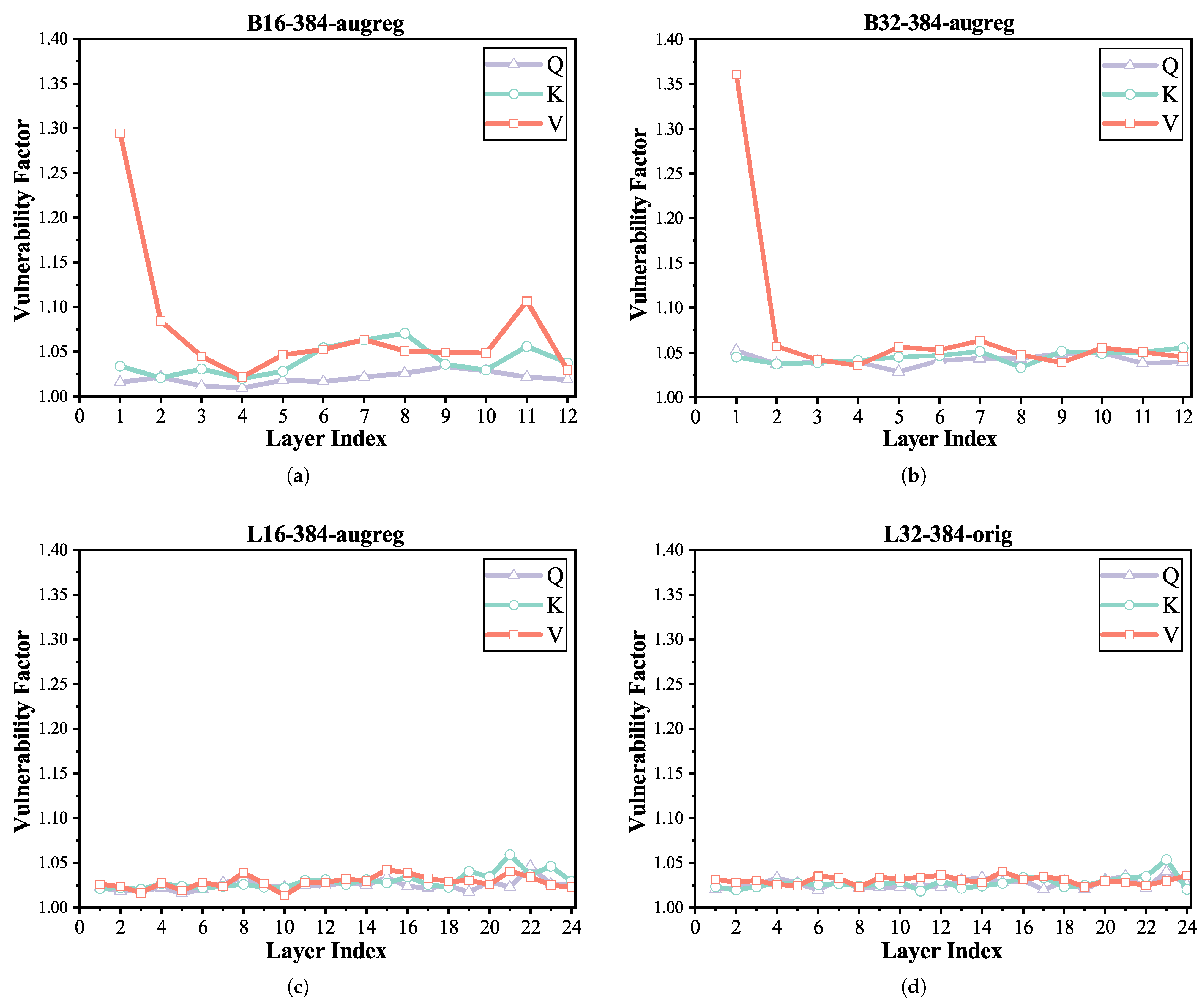
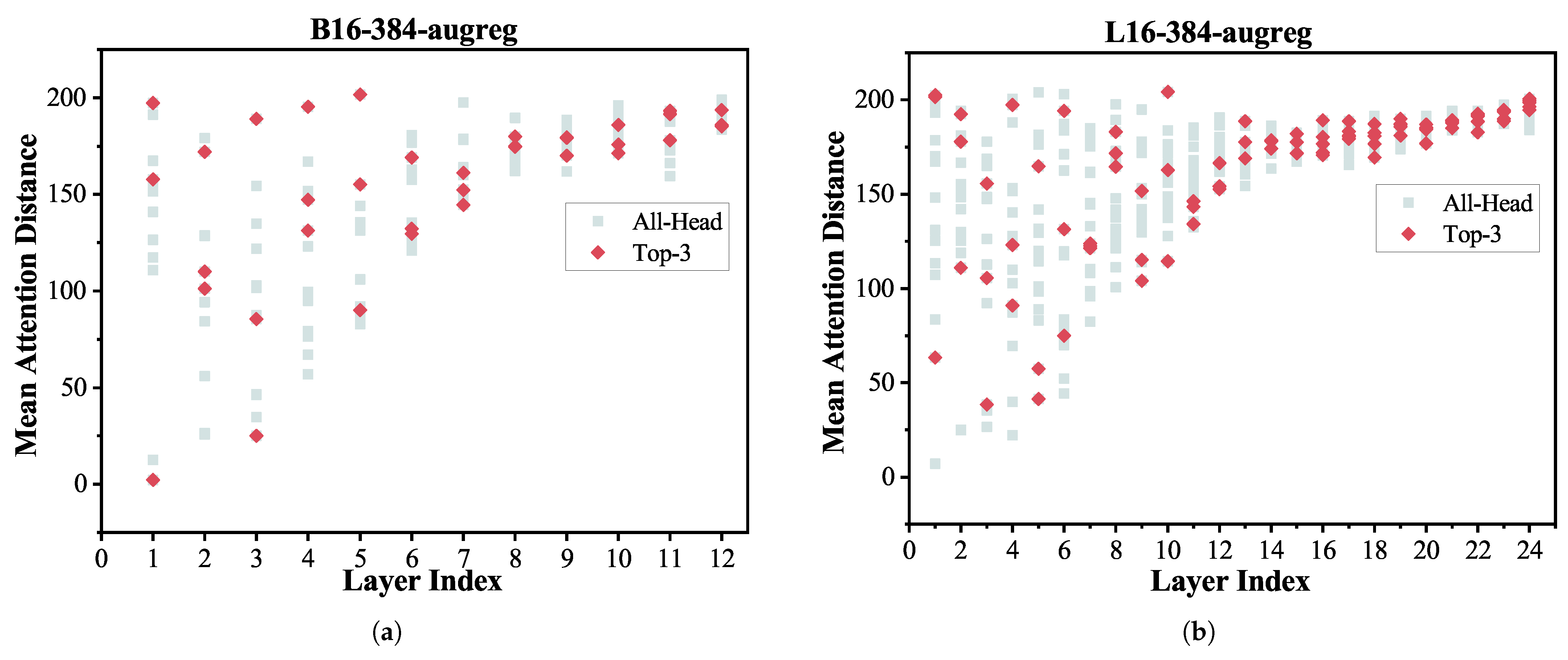
• In the type-wise and head-wise analyses, we revealed heterogeneous vulnerability patterns across Q, K, and V projection matrices and attention heads. Notably, we integrated the mean attention distance (MAD) metric to interpret why certain heads are more fault-prone—an interpretability perspective not addressed in previous works.

2. ViT Model and Fault Resilience Evaluation Platform

2.1. ViT Model

The transformer architecture [9] overcomes the challenge of capturing non-local dependencies faced by traditional NLP models by introducing the self-attention mechanism. Inspired by the huge success of the transformer in NLP, ViT is designed to apply the original transformer architecture for image classification tasks as closely as possible [12]. Leveraging scalable NLP transformer architectures and their efficient implementations, ViT achieves classification accuracy that surpasses state-of-the-art (SOTA) performance. A classical ViT architecture consists of three main components: patch embedding, transformer encoder, and MLP head. The transformer encoder is composed of alternating layers of multi-headed self-attention (MSA) and MLP blocks, as shown in Figure 1. Compared to the original transformer, layer norm (LN) is applied before the MSA and MLP block for better performance.

To receive 2D images, ViT changes the input image $\mathbf{x}\in {\mathbb{R}}^{H\times W\times C}$ into a sequence of flattened 2D patches ${\mathbf{x}}_p\in {\mathbb{R}}^{N\times (P^2·C)}$, where $(H, W)$ is the height and width of the input image, C is the number of channels, $(P, P)$ is the resolution of each image patch, e.g., $16\times 16$ in ViT original paper, and $N=HW/P^2$ is the number of patches. ViT flattens each patch and uses a trainable linear projection to map it to the D dimension, which is the constant latent vector size used in the transformer through all of its layers:

$$\mathbf{I}=({\mathbf{x}}_p^1\mathbf{E};{\mathbf{x}}_p^2\mathbf{E};\dots ;{\mathbf{x}}_p^N\mathbf{E}),\mathbf{E}\in {\mathbb{R}}^{(P^2·C)\times D}$$

(1)

ViT attaches a learnable embedding (${\mathbf{x}}_{class}$) to the sequence of embedded patches, which is used at the output of the encoder to serve as the image representation. Position embeddings are added to the patch embeddings to keep the image positional information:

$${\mathbf{z}}_0=[{\mathbf{x}}_{class};\mathbf{I}]+{\mathbf{E}}_{pos},{\mathbf{E}}_{pos}\in {\mathbb{R}}^{(N+1)\times D}$$

(2)

The embedded patches ($\mathbf{z}$) will then pass through LN and MSA. The self-attention (SA) relies on a scaled dot-product attention, which operates on a query matrix $\mathbf{Q}$, a key matrix $\mathbf{K}$, and a value matrix $\mathbf{V}$. For each element in an input sequence $\mathbf{z}\in {\mathbb{R}}^{N\times D}$, ViT computes a weighted sum over all values $\mathbf{v}$ in the following sequence:

$$[\mathbf{Q}, \mathbf{K}, \mathbf{V}]=\mathrm{LN}\left(\mathbf{z}\right){\mathbf{U}}_{qkv},{\mathbf{U}}_{qkv}\in {\mathbb{R}}^{D\times 3D_h}$$

(3)

$$\mathrm{SA}(\mathbf{Q}, \mathbf{K}, \mathbf{V})=\mathbf{V} \times \mathrm{softmax}\left({\displaystyle \frac{{\mathbf{K}}^{\top }\mathbf{Q}}{\sqrt{D^h}}}\right)$$

(4)

MSA is an extension of SA in which it calculates k self-attention operations in parallel and projects concatenated outputs to keep each layer with the same size:

$$\mathrm{MSA}\left(\mathbf{z}\right)=[{\mathrm{SA}}_1\left(\mathrm{z}\right);{\mathrm{SA}}_2\left(\mathrm{z}\right);\dots ;{\mathrm{SA}}_{\mathrm{k}}\left(\mathrm{z}\right)]{\mathbf{U}}_{msa},{\mathbf{U}}_{msa}\in {\mathbb{R}}^{k·D_h\times D}$$

(5)

After the residual addition, the input of the MLP is

$${\mathbf{z}}_{\ell }^{\prime }=\mathrm{MSA}\left(\mathrm{LN}\left({\mathbf{z}}_{\ell -1}\right)\right)+{\mathbf{z}}_{\ell -1},\ell =1\dots L$$

(6)

MLP is composed of two fully connected layers and a nonlinear activation function between them. After the residual normalization and addition, the output of the encoder is as follows:

$${\mathbf{z}}_{\ell }=\mathrm{MLP}\left(\mathrm{LN}\left({\mathbf{z}}_{\ell }^{\prime }\right)\right)+{\mathbf{z}}_{\ell }^{\prime },\ell =1\dots L$$

(7)

which has the same dimension as the input, so it can be passed to the input of the next encoder directly. The dimensions of various weight matrices in different ViT variants are summarized in

Table 1. Dimensions of different weight matrices in different ViT models.

Model Variant	Component Name	Weight Category	Weight Dimension
ViT-B/16	patch embedding	cls_token	$1\times 1\times 768$
		pos_embed	$1\times 577\times 768$
		patch_embed	$768\times 3\times 16\times 16$
	encoder layer1~12	attn.qkv	$2304\times 768$
		attn.proj	$768\times 768$
		mlp.fc1	$3072\times 768$
		mlp.fc2	$768\times 3072$
	classification head	head	$768\times 1000$
ViT-B/32	patch embedding	cls_token	$1\times 1\times 768$
		pos_embed	$1\times 145\times 768$
		patch_embed	$768\times 3\times 32\times 32$
	encoder layer1~12	attn.qkv	$2304\times 768$
		attn.proj	$768\times 768$
		mlp.fc1	$3072\times 768$
		mlp.fc2	$768\times 3072$
	classification head	head	$768\times 1000$
ViT-L/16	patch embedding	cls_token	$1\times 1\times 1024$
		pos_embed	$1\times 577\times 1024$
		patch_embed	$1024\times 3\times 16\times 16$
	encoder layer1~24	attn.qkv	$3072\times 1024$
		attn.proj	$1024\times 1024$
		mlp.fc1	$4096\times 1024$
		mlp.fc2	$1024\times 4096$
	classification head	head	$1024\times 1000$
ViT-L/32	patch embedding	cls_token	$1\times 1\times 1024$
		pos_embed	$1\times 145\times 1024$
		patch_embed	$1024\times 3\times 32\times 32$
	encoder layer1~24	attn.qkv	$3072\times 1024$
		attn.proj	$1024\times 1024$
		mlp.fc1	$4096\times 1024$
		mlp.fc2	$1024\times 4096$
	classification head	head	$1024\times 1000$

. ViT architecture is generally composed of three fundamental components: patch embedding, encoder layer, and classification head. In the patch embedding component, there are three kinds of weight matrices: a learnable clk_token to aggregate the global representation of the input image, a pos_embed to incorporate information about the spatial positions of patches, and a patch_embed converting the input image into a sequence of flattened and projected 2D patches. Within the encoder layer component, the specific parameter types—such as attention and MLP sub-modules—are detailed in Figure 1. In the classification head component, the head is a fully connected layer that maps the final output of the cls_token to the logits corresponding to each target class. It serves as the output layer for classification.

2.2. Fault Resilience Evaluation Platform

2.2.1. Soft Errors

Inspired by ViT’s remarkable accuracy, many studies have attempted to employ ViT in safety-critical missions like automotive, space, and industry to extract useful information from complex raw data [34]. Hence, the dependability of deployed accelerator-based systems (e.g., GPU or DNN accelerator) is of paramount importance. Their failure can result in catastrophic consequences [35]. Moreover, with the continuous scaling of CMOS technology feature size and the lowering voltage of large-scale VLSI designs, soft errors have become inevitable. Soft error is a type of transient error that temporarily corrupts data without causing permanent damage to the hardware. It is typically caused by external interface, such as high-energy neutron or alpha particle strikes. Soft errors usually affect only one bit of data, flipping it from 1 to 0 or from 0 to 1 in SRAM, registers, or flip-flops, so the bit-flip error was utilized to model soft errors in fault simulation [20,21]. We will utilize soft errors or bit-flip errors interchangeably throughout this article. The soft errors can corrupt the data stored in memory and propagate along with the hardware data flow, spread to more operations, and generate incorrect computing results, which may induce considerable prediction accuracy loss of deep learning models.

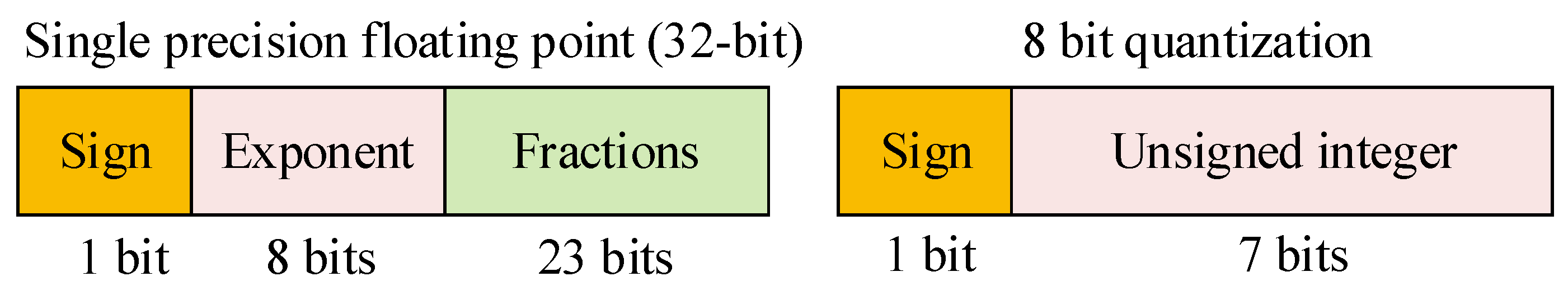
2.2.2. Quantization

Quantization is a widely adopted model compression technique that reduces the computational and memory footprint of DNNs by mapping high-precision floating-point values to lower-precision fixed-point representations. This process enables efficient inference on resource-constrained hardware, such as edge devices and embedded systems, without significantly compromising model accuracy [36,37,38]. Among the various quantization schemes, post-training quantization and quantization-aware training are commonly used to transform model weights and activations from 32-bit floating-point (FP32) to 8-bit integer (Int8) formats. As shown in Figure 2, the FP32 format, as defined by the IEEE 754 standard [39], consists of 1 sign bit, 8 exponent bits, and 23 mantissa (fraction) bits, allowing for a wide dynamic range and high numerical precision. In contrast, the Int8 format represents data using a fixed 8-bit signed integer, typically ranging from −128 to 127.

To enable accurate mapping between FP32 and Int8 representations, quantization relies on $scale$ factors and $\mathit{zero\_point}$ to calibrate the distribution of floating-point values within the limited range of integers. This transformation from FP32 to Int8 can be written as follows:

$$x_q=\mathrm{Clip}\left(\mathrm{Round}({\displaystyle \frac{x_f}{scale}}+\mathit{zero\_point})\right)$$

(8)

where $x_q$ is the original floating-point value, and $x_f$ represents the quantized integer result. $\mathit{zero\_point}$ is an integer offset that aligns the zero value of the floating-point domain with that of the quantized domain. $\mathrm{Round}(·)$ applies standard rounding to the nearest integer. $\mathrm{Clip}(·)$ ensures the quantized output is bounded within the target range, typically $[-128, 127]$ for 8-bit signed integers. $scale$ is a positive scaling factor that can be calculated as follows:

$$scale={\displaystyle \frac{x_{max}-x_{min}}{Q_{max}-Q_{min}}}$$

(9)

Here, $x_{max}$ and $x_{min}$ represent the maximum and minimum values in the distribution of weights or activations. $Q_{max}$ and $Q_{min}$ denote the upper and lower bounds of the quantized integer range, respectively. Dequantization can be easily written as follows:

$$x_f=scale·(x_q-\mathit{zero\_point})$$

(10)

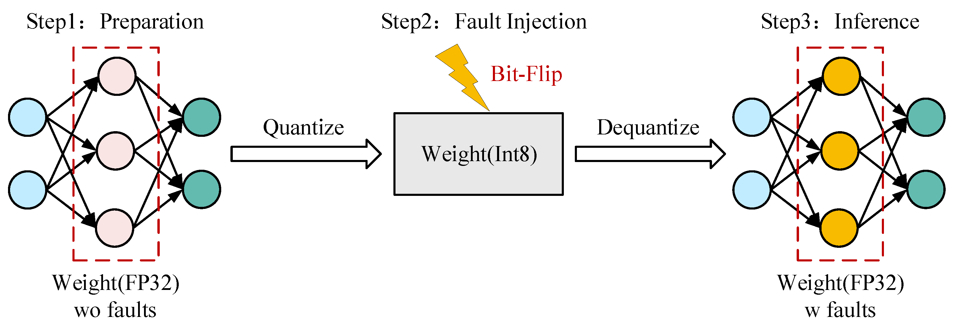
2.2.3. Fault Injection Method

In this paper, we mainly focus on bit-flip errors in memory, which are pertinent to ViT due to the large storage requirement for weights and intermediate states. In prior work, Ares by Reagen et al. [40] offers a fault resilience evaluation platform for DNN models based on PyTorch. Ares targets custom hardware implementations and establishes a complete resilience evaluation flow from training to fault injection. Our fault resilience evaluation platform has several extensions compared to Ares, and the differences are summarized in

Table 2. Comparison between Ares and our improved approach.

	Ares	Our Extensions
Quantization Method	Fixed-Point Quantization	Integer Quantization (Int16, Int8, Int4)
Support Models	Classical CNNs (e.g., NLP, LeNet, AlexNet, VGG, etc.)	Different kinds of ViTs (e.g., original ViTs, Swin Transformer, and DeepViT)
Different Architecture Granularity	Model-wise, Layer-wise	Type-wise, Head-wise

.

The overall fault injection workflow consists of three main steps, namely preparation, fault injection, and inference, as shown in Figure 3:

• Given the original 32-bit floating-point weights ${\mathrm{W}}_{\mathtt{\text{FP32}}}$, we first apply post-training quantization to obtain the 8-bit integer representation ${\mathrm{W}}_{\mathtt{Int8}}$:

  $${\mathtt{W}}_{\mathtt{Int8}}=\mathrm{Quantize}\left({\mathrm{W}}_{\mathtt{FP32}}\right)$$

  (11)

  where the $\mathrm{Quantize}(·)$ function is defined at (8).
• Bit-flip faults are injected directly into the quantized integer weights:

  $${\mathrm{W}}_{\mathtt{Int8}}^{Fault}=\mathrm{BitFlip}({\mathrm{W}}_{\mathtt{Int8}},\mathcal{F})$$

  (12)

  where $\mathcal{F}$ represents the injected fault mask.
• The corrupted integer weights are then dequantized back to floating-point format:

  $${\mathbf{W}}_{\mathtt{FP32}}^{Fault}=\mathrm{Dequantize}\left({\mathbf{W}}_{\mathtt{Int8}}^{Fault}\right)$$

  (13)

  $$\widehat{\mathbf{y}}=\mathcal{M}(\mathbf{x};{\mathbf{W}}_{\mathtt{FP32}}^{Fault})$$

  (14)

  where the $\mathrm{Dequantize}(·)$ function is defined at (10), $\mathbf{x}$ is the model input, $\mathcal{M}$ is the target ViT model, and $\widehat{\mathbf{y}}$ is the model output prediction.

3. Results

3.1. Experimental Setup

We conducted fault simulation experiments on a GPU server equipped with an Intel Xeon Gold 6253CL CPU, 500GB of RAM, and two NVIDIA Tesla V100 GPUs (totaling 64GB of global memory), using CUDA 12.4, PyTorch 2.5.1, and Python 3.7. Seven different ViT models from the HuggingFace timm library (v1.0.12) were evaluated by performing inference on randomly selected image batches from the ImageNet dataset. All models belonged to the Original ViT with different blocks and input patches.

Table 3. Summary of ViT variants: names, patch sizes, block counts, accuracy, and size of parameters.

Model Name *	Input Size	Patches	Layers	Accuracy (%)	Size (MB)
B16-224-augreg	$224\times 224$	16	12	84.536%	330
B16-384-augreg	$384\times 384$	16	12	85.998%	330
B32-224-augreg	$224\times 224$	32	12	80.718%	336
B32-384-augreg	$384\times 384$	32	12	83.350%	336
L16-384-augreg	$384\times 384$	16	24	87.098%	1160
L32-384-orig	$384\times 384$	32	24	81.512%	1169
H14-224-orig **	$224\times 224$	14	32	88.272%	2410

* We use brief notation to indicate the model size, input patch size, and input image size: for instance, B16-384 means the “Base” variant with 16 × 16 input patch size and 384 × 384 input image size. ** “orig” means trained with normal methods. “augreg” means trained with additional augmentation and regularization.

shows the essential features of the evaluated models, including their model names, the number of input patches, the number of layers, accuracy, and parameter size.

In our experiments, we adopted two fault injection methodologies to enable multi-granularity analyses. The first approach applied a range of bit error rates (BERs) on a logarithmic scale for model-wise evaluation, while the second method employed fixed BER values for type-wise, layer-wise, and head-wise analysis. The BER denotes the fraction of total integer weight bits that are randomly selected and flipped. To evaluate the model’s robustness under different fault tolerance requirements, we defined the 0%, 1%, 5%, and 10% accuracy loss BER thresholds as the BER at which the model’s classification error increased by no more than 0, 1, 5, and 10 percentage points, respectively, compared to its reference performance. These thresholds reflect varying levels of robustness: A higher 0% accuracy loss threshold means that the model can tolerate more errors without loss of accuracy, while the 1% accuracy loss threshold indicates near-error-free resilience suitable for safety-critical scenarios; the 5% threshold represents moderate degradation acceptable in non-critical applications; and the 10% threshold corresponds to substantial accuracy loss, marking a limit beyond which the model’s predictions become unreliable without additional protection mechanisms. A higher BER threshold means that the model can tolerate more errors without loss of accuracy. To quantify the reliability of different components within ViT models, we introduced the vulnerability factor as a metric, defined as the accuracy degradation between the fault-injected model and its counterpart.

To ensure the statistical robustness of the results, each experiment was performed through ten independent injection trials, each initialized with a different random seed. The number of iterations was selected to balance computational cost and result stability and enabled the reporting of mean, standard deviation, and worst-case accuracy under fault conditions. The error bars for all the experimental results were calculated based on 95% confidence intervals.

We took the following steps in performing our experiments:

• Load original models from HuggingFace and record the models’ original accuracy.
• Quantize specific (or all) layer weight parameters by converting them into integer data types.
• Initiate fault injection on the specified layers and distribute the corresponding computation jobs across multiple GPUs.
• Record the inference accuracy of the fault-injected models on the ImageNet-1k validation set.
• Repeat steps 1 through 4 ten times, and record the average, standard deviation, maximum, and minimum accuracy for each model.

Table 4. Execution time required for preparation and different ViT fault injection experiments.

Preparation 1	Model-Wise	Layer-Wise	Type-Wise	Head-Wise
≈0 h 2	10 h	5 h	2 h	25 h

¹ Preparation consists of recording original accuracy, weight quantization, and fault injection. ² It is negligible compared to the execution time of other experiments.

summarizes the execution time required to complete various fault injection experiments by running two concurrent processes per GPU. The head-wise experiment incurred the highest time cost due to the large number of attention heads (typically ranging from 12 heads in the ViT base model to 16 heads in the ViT large model) in each model.

3.2. Results and Analysis

3.2.1. Model-Wise

In our model-wise experiments, we considered a range of BERs from ${10}^{-8}$ to ${10}^{-2}$ for fault injection across all possible layers, using the first injection method, as mentioned in Section 3.1. Figure 4 illustrates the impact of BERs on classification error for different ViT models. The x-axis represents the BER on a logarithmic scale, while the y-axis represents the classification error. Each subplot corresponds to a different ViT model, showing how their classification performance degraded as the BER increased. A red dashed vertical line indicates the 0% accuracy loss BER threshold, which is defined as the highest BER at which the model’s classification error is not higher than its original error. These results show that model size and patch size may influence the error resilience of ViT models. Different models’ BER thresholds can span several orders of magnitude.

Table 5. ViT models at 1%, 5%, and 10% accuracy loss BER thresholds.

Model	1% Accuracy Loss	5% Accuracy Loss	10% Accuracy Loss
B16-224-augreg	$4.062\times {10}^{-6}$	$2.015\times {10}^{-5}$	$3.675\times {10}^{-5}$
B16-384-augreg	$4.062\times {10}^{-6}$	$1.650\times {10}^{-5}$	$3.008\times {10}^{-5}$
B32-224-augreg	$6.062\times {10}^{-6}$	$3.008\times {10}^{-5}$	$5.484\times {10}^{-5}$
B32-384-augreg	$1.650\times {10}^{-5}$	$5.484\times {10}^{-5}$	$10.000\times {10}^{-5}$
L16-384-augreg	$5.484\times {10}^{-5}$	$1.823\times {10}^{-4}$	$2.721\times {10}^{-4}$
L32-384-orig	$2.015\times {10}^{-5}$	$1.000\times {10}^{-4}$	$1.823\times {10}^{-4}$

presents the accuracy loss across different models at various BER thresholds, specifically when the classification error loss reached 1%, 5%, and 10%. The general trend is that larger models with smaller patches tend to be more robust, while all models’ errors increase significantly beyond a certain threshold of BER. These trends are consistent with the data collected through more than 70 h of neutron beam experiments [19].

3.2.2. Layer-Wise

In this section, the importance of individual layers in different ViT models is evaluated by introducing the same BER. Each layer in a ViT model consists of multiple sub-blocks, as outlined in Table 1, such as the attn.qkv, attn.proj, mlp.fc1 and mlp.fc2. According to the settings of BER, we randomly selected weights from the weight matrices of these sub-blocks, such as $W_{qkv}$, $W_{proj}$, $W_{FC1}$, and $W_{FC2}$ and injected bit-flip faults to the chosen weights; then, we ran the model and determined the classification accuracy with errors. This scenario was repeated 10 times for each layer from the first to the last, and the average vulnerability factor was used to quantify the sensitivity of each layer to weight perturbations.

The results are shown in the bar chart in Figure 5, revealing several noteworthy observations. The bar charts represent the vulnerability factors obtained via fault injection for two model variants, while the dotted line plots show the results from the identity replacement experiment. For B16-384-augreg and B32-384-augreg, both of which consist of 12 layers, the vulnerability factors remain significantly high, with an average of 5.376 and 4.339, respectively, particularly in the early (Layers 1~2) and middle stages (Layers 3~9). In contrast, L16-384-augreg and L32-384-orig, with 24 layers, show much lower vulnerability factors. However, the first few layers (Layers 1-2) of these models exhibit relatively higher vulnerability factors than the other layers. These observations indicate that certain layers within the model contribute differently to its overall accuracy. Some layers are more critical than others. To validate this assumption, we conducted an experiment in which the selected layers of the model were replaced with torch.nn.Identity(), a placeholder identity operator that simply returns its input without any transformation, in order to assess the contribution of each layer to the overall inference accuracy. As shown in the dotted line plot in Figure 5, the identity experiment results exhibit a similar trend to that observed in the layer-wise fault injection experiments, where the first layer and the layers close to the output (Layers 8~9) show notably higher sensitivity.

To gain a deeper understanding of how sub-blocks within each layer (e.g., attn.qkv, attn.proj, mlp.fc1, and mlp.fc2 affect its vulnerability), we conducted targeted fault injection experiments on each sub-block individually. The fine-grained vulnerability analysis of individual sub-blocks is shown in Figure 6. For the B16-384-augreg model, the attn.proj in the initial layer, along with the mlp.fc1 and mlp.fc2 components in Layers 4 through 9, exhibit a higher contribution to layer-wise vulnerability. For the L32-384-orig model, the attn.proj module, as well as both mlp.fc1 and mlp.fc2, demonstrate notable sensitivity in the first layer. Consistent with observations from the B16-384-augreg model, the MLP components exhibit greater sensitivity in the intermediate and deeper layers.

The early layers in a ViT primarily focus on capturing local and low-level features, such as fine-grained textures, edges, and local patterns, from the input image. As the input is divided into non-overlapping patches and projected into an embedding space, these shallow layers refine the token representations through self-attention and feed-forward operations. Consequently, the attn.proj sub-block in the first layer of both models is much more important than the other components due to its fundamental role in initial feature extraction from input patches through the attention mechanism. As the network progresses, deeper layers increasingly focus on global context modeling and high-level feature abstraction. The model relies on mlp.fc1 and mlp.fc2 in the middle and deeper layers to enhance its nonlinear representation capacity, facilitating the recognition of a wider variety of images and supporting more accurate classification outcomes.

To further investigate this phenomenon observed in L16-384-augreg and L32-384-orig, we conducted the same experiments on a deeper model, H14-224-orig, and the results in Figure 7 show that deeper models exhibit more sensitivity at the first layer.

3.2.3. Type-Wise

In this part of the study, we systematically injected faults into the projection matrices of the query (Q), key (K), and value (V) components at each layer within the attn.qkv sub-block to assess the impact of different weight matrix types on overall model accuracy. As shown in (3), a single linear transformation (fully connected layer) can be applied to compute Q, K, and V simultaneously, so the size of attn.qkv is $3(N+1)\times D$, where $N+1$ represents the length of input patches plus a $\mathit{clk\_token}$, and D stands for the dimension of each 1-D patch. For each simulation, the weight matrix attn.qkv was divided into three parts ($W_Q$, $W_K$, $W_V$), and a weight parameter was selected from one of these three matrices (e.g., $W_Q$) at a designated layer (e.g., layer-x). The model was then executed 10 times to assess the effect of errors on $W_Q$ in layer-x. Figure 8 presents the vulnerability factor of the Q, K, and V projection matrices across different layers for various model configurations. For the B16-384-augreg model with a 384-dimensional embedding and augmentation-based regularization, a notable peak in the vulnerability factor of the V matrix was observed at the first layers. Under the same conditions, the B32-384-augreg model showed a similar trend where the V matrix exhibited heightened vulnerability among the three projection matrices in the initial layers. This heightened sensitivity can be attributed to the role of the V matrix in directly shaping the attention outputs, as shown in (4). Unlike the Q and K matrices, which determine attention weights through similarity computation, the V matrix transforms the actual content that is propagated through the self-attention mechanism. Therefore, faults in the V matrix may have a more immediate and amplified effect on the resulting feature representations. The trend diminishes in later layers, and this phenomenon is similar to the trend in Section 3.2.2. For L16-384-augreg and L32-384-orig models, the vulnerability factors for Q, K, and V remain close to 1 across all layers, indicating a more uniform distribution of sensitivity. This phenomenon can be attributed to the relatively low vulnerability factor observed in ViT Large models. These results indicate that ViT Large models have much less reliance on the attn.qkv sub-block, particularly in the first layer, as shown in Figure 6b.

3.2.4. Head-Wise

Multi-head attention projects the input into multiple subspaces, allowing each head to learn different feature patterns, such as local edge details and global shape structures. Since different attention heads independently focus on different parts of the input, the model can learn more comprehensive representations. To further investigate the resilience of different attention heads, we performed fault injections on different attention heads separately. Figure 9 shows that different attention heads exhibit varying degrees of sensitivity, particularly in the first layer. This observation implies that certain heads are functionally more significant, potentially playing a pivotal role in the model’s inferential processes.

To further investigate and understand how different heads in different layers affect the models’ accuracy, we calculated the mean attention distance (MAD) [12] of the three most vulnerable attention heads in each layer. The MAD refers to the average spatial distance (pixels or patches) between a given query patch and the key patches it attends to in the self-attention mechanism. It quantifies how “far” the model’s attention head looks when aggregating information across the input image.

The results are shown in Figure 10. In this figure, the gray dots represent the MAD values of all original attention heads, while the red dots indicate the MAD values of the top three most sensitive heads. We can infer that the top three most sensitive head covers both have large and small attention distances in each layer. A key factor underlying the success of ViTs is the incorporation of self-attention, which allows the model to capture information across the entire image patches, even in the lowest layers. This phenomenon indicates that attention heads responsible for capturing both local and global contextual information from image patches play equally important roles in the model’s inference process.

Table 6. The MAD of Top-5 sensitive heads.

Model Name	Layer 1, Head X *	Vulnerability Factor	Mean Attention Distance
B16-384-augreg	7	5.1096	157.72
	4	3.9056	2.15
	10	2.6086	197.26
	1	2.6037	151.55
	0	2.0893	12.50
L16-384-augreg	14	1.1614	63.31
	8	1.1354	202.58
	15	1.1342	201.59
	6	1.1042	148.32
	13	1.0834	167.17

* Sorted in descending order based on vulnerability factor.

presents the MAD values of the five most sensitive attention heads in the first layer across the two models.

These findings offer valuable guidance for both architectural refinement and accelerator fault-tolerant design. For instance, MAD can be used as a heuristic to selectively harden or replicate attention heads that span broader distances, which may be more functionally significant. Moreover, model pruning or quantization strategies should be MAD-aware to avoid disproportionately impacting attention diversity and spatial coverage. By incorporating MAD into the design loop, more resilient and computation-efficient ViT architectures may be achieved.

4. Conclusions

This paper presents a fine-grained vulnerability analysis of various ViT variants using two kinds of bit-flip fault injection methods. The analysis was conducted from four perspectives: model-wise, layer-wise, type-wise, and head-wise. The model-wise experimental results show that model size and patch size may influence the error resilience of ViT models. Different models’ BER thresholds can span several orders of magnitude. For layer-wise, type-wise, and head-wise experiments, the results can be summarized as follows: (1) Due to its crucial role in extracting both local and global features from input patches, the first layer exhibits high sensitivity to faults for both ViT base and large models, with errors in this layer leading to substantial degradation in model inference accuracy. (2) In the middle and later stages of the ViT model, the mlp.fc1 and mlp.fc2 sub-blocks within each layer play a dominant role in the overall computation and representation learning. Faults in these sub-blocks in the middle and later stages of the ViT model can result in a considerable reduction in inference accuracy. (3) In contrast to intuitive expectations, attention heads responsible for capturing both local and global contextual information from image patches equally contribute to the model’s inference process. Given the high sensitivity of the first transformer, patches, fault-tolerant design techniques such as error correction codes (ECCs), triple modular redundancy (TMR), or selective use of higher-precision data formats (e.g., FP16 instead of Int8) can be employed to enhance reliability. Additionally, robustness-aware training strategies, including noise injection or adversarial perturbation targeting the first layer, may improve its fault resilience during inference. In future work, we intend to utilize these findings to inform the development of more efficient and fault-tolerant hardware accelerators specifically designed for ViT models. Additionally, we aim to develop theoretical models and mathematical formulations to better explain and predict the fault sensitivity patterns observed in this study. Our proposed fault sensitivity analysis and mitigation strategies for ViTs are particularly applicable to safety-critical systems, where robustness against hardware faults is essential. For instance, in autonomous vehicles, aerospace guidance systems, and industrial robotics, even minor computation errors can lead to severe system failures. The ability to identify and harden vulnerable components of ViT models could enhance the deployment of deep learning systems in these domains by improving their reliability and fault tolerance.

References

- Krizhevsky, A.; Sutskever, I.; Hinton, G.E. ImageNet classification with deep convolutional neural networks. Commun. Acm 2017, 60, 84–90. [Google Scholar] [CrossRef]
- Szegedy, C.; Liu, W.; Jia, Y.; Sermanet, P.; Reed, S.; Anguelov, D.; Erhan, D.; Vanhoucke, V.; Rabinovich, A. Going deeper with convolutions. In Proceedings of the IEEE Conference on Computer Vision and Pattern Recognition (CVPR), Boston, MA, USA, 7–12 June 2015; pp. 1–9. [Google Scholar] [CrossRef]
- He, K.; Zhang, X.; Ren, S.; Sun, J. Deep residual learning for image recognition. In Proceedings of the IEEE Conference on Computer Vision and Pattern Recognition (CVPR), Las Vegas, NV, USA, 27–30 June 2016; pp. 770–778. [Google Scholar] [CrossRef]
- Howard, A.G.; Zhu, M.; Chen, B.; Kalenichenko, D.; Wang, W.; Weyand, T.; Andreetto, M.; Adam, H. MobileNets: Efficient Convolutional Neural Networks for Mobile Vision Applications. arXiv 2017, arXiv:1704.04861. [Google Scholar]
- Mikolov, T.; Chen, K.; Corrado, G.; Dean, J. Efficient Estimation of Word Representations in Vector Space. arXiv 2013, arXiv:1301.3781. [Google Scholar]
- Pennington, J.; Socher, R.; Manning, C.D. GloVe: Global Vectors for Word Representation. In Proceedings of the 2014 Conference on Empirical Methods in Natural Language Processing (EMNLP), Doha, Qatar, 25–29 October 2014. [Google Scholar] [CrossRef]
- Cho, K.; van Merriënboer, B.; Gulcehre, C.; Bahdanau, D.; Bougares, F.; Schwenk, H.; Bengio, Y. Learning Phrase Representations using RNN Encoder–Decoder for Statistical Machine Translation. arXiv 2014, arXiv:1406.1078. [Google Scholar] [CrossRef]
- Huang, Z.; Xu, W.; Yu, K. Bidirectional LSTM-CRF models for sequence tagging. arXiv 2015, arXiv:1508.01991. [Google Scholar]
- Vaswani, A.; Shazeer, N.; Parmar, N.; Uszkoreit, J.; Jones, L.; Gomez, A.N.; Kaiser, Ł.; Polosukhin, I. Attention is all you need. In Proceedings of the Advances in Neural Information Processing Systems (NeurIPS), Long Beach, CA, USA, 4–9 December 2017. [Google Scholar]
- Elman, J.L. Finding structure in time. Cogn. Sci. 1990, 14, 179–211. [Google Scholar] [CrossRef]
- Hochreiter, S.; Schmidhuber, J. Long short-term memory. Neural Comput. 1997, 9, 1735–1780. [Google Scholar] [CrossRef] [PubMed]
- Dosovitskiy, A.; Beyer, L.; Kolesnikov, A.; Weissenborn, D.; Zhai, X.; Unterthiner, T.; Dehghani, M.; Minderer, M.; Heigold, G.; Gelly, S.; et al. An Image is Worth 16x16 Words: Transformers for Image Recognition at Scale. In Proceedings of the International Conference on Learning Representations (ICLR), Vienna, Austria, 4 May 2021. [Google Scholar] [CrossRef]
- Carion, N.; Massa, F.; Synnaeve, G.; Usunier, N.; Kirillov, A.; Zagoruyko, S. End-to-End Object Detection with Transformers. In Proceedings of the European Conference on Computer Vision (ECCV), Glasgow, UK, 23–28 August 2020. [Google Scholar] [CrossRef]
- Devlin, J.; Chang, M.W.; Lee, K.; Toutanova, K. BERT: Pre-training of Deep Bidirectional Transformers for Language Understanding. arXiv 2018, arXiv:1810.04805. [Google Scholar]
- Touvron, H.; Cord, M.; Douze, M.; Massa, F.; Sablayrolles, A.; Jégou, H. Training data-efficient image transformers & distillation through attention. In Proceedings of the 38th International Conference on Machine Learning, Virtual, 18–24 July 2021; Volume 139, pp. 10347–10357. [Google Scholar]
- Wu, H.; Xiao, B.; Codella, N.; Liu, M.; Dai, X.; Yuan, L.; Zhang, L. Cvt: Introducing convolutions to vision transformers. In Proceedings of the IEEE/CVF International Conference on Computer Vision (ICCV), Montreal, QC, Canada, 10–17 October 2021; pp. 22–31. [Google Scholar] [CrossRef]
- Wortsman, M.; Ilharco, G.; Gadre, S.Y.; Roelofs, R.; Gontijo-Lopes, R.; Morcos, A.; Namkoong, H.; Farhadi, A.; Carmon, Y.; Kornblith, S.; et al. Model soups: Averaging weights of multiple finetuned models improves accuracy without increasing inference time. In Proceedings of the International Conference on Machine Learning, Baltimore, MD, USA, 17–23 July 2022; pp. 23965–23998. [Google Scholar]
- Han, K.; Wang, Y.; Guo, J.; Tang, Y.; Chen, E.; Xu, C.; Xu, C.; Tao, D. Transformers in Vision: A Survey. IEEE Trans. Pattern Anal. Mach. Intell. (TPAMI) 2023, 45, 87–110. [Google Scholar] [CrossRef] [PubMed]
- Roquet, L.; Fernandes dos Santos, F.; Rech, P.; Traiola, M.; Sentieys, O.; Kritikakou, A. Cross-Layer Reliability Evaluation and Efficient Hardening of Large Vision Transformers Models. In Proceedings of the DAC ’24: 61st ACM/IEEE Design Automation Conference, New York, NY, USA, 23–27 June 2024; pp. 1–6. [Google Scholar] [CrossRef]
- Baumann, R.C. Radiation-induced soft errors in advanced semiconductor technologies. IEEE Trans. Device Mater. Reliab. 2005, 5, 305–316. [Google Scholar] [CrossRef]
- Bernstein, K.; Rohrer, N.J.; Nowak, E.; Carrig, B.; Durham, C.; Hansen, P.; Smalley, D.; Streeter, S. Designing reliable systems from unreliable components: The challenges of transistor variability and degradation. Ibm J. Res. Dev. 2006, 50, 455–467. [Google Scholar] [CrossRef]
- Li, G.; Hari, S.K.S.; Sullivan, M.; Tsai, T.; Pattabiraman, K.; Emer, J.; Keckler, S.W. Understanding Error Propagation in Deep Learning Neural Network (DNN) Accelerators and Applications. In Proceedings of the SC ’17: International Conference for High Performance Computing, Networking, Storage and Analysis, New York, NY, USA, 12–17 November 2017; pp. 1–12. [Google Scholar] [CrossRef]
- Hong, S.; Frigo, P.; Kaya, Y.; Giuffrida, C.; Dumitras, T. Terminal Brain Damage: Exposing the Graceless Degradation in Deep Neural Networks Under Hardware Fault Attacks. In Proceedings of the 28th USENIX Security Symposium (USENIX Security 19), Santa Clara, CA, USA, 4–16 August 2019; pp. 497–514. [Google Scholar]
- Sabbagh, M.; Gongye, C.; Fei, Y.; Wang, Y. Evaluating Fault Resiliency of Compressed Deep Neural Networks. In Proceedings of the 2019 IEEE International Conference on Embedded Software and Systems (ICESS), Las Vegas, NV, USA, 2–3 June 2019; pp. 1–7. [Google Scholar] [CrossRef]
- Xu, D.; Chu, C.; Wang, Q.; Liu, C.; Wang, Y.; Zhang, L.; Liang, H.; Cheng, K.T. A Hybrid Computing Architecture for Fault-tolerant Deep Learning Accelerators. In Proceedings of the 2020 IEEE 38th International Conference on Computer Design (ICCD), Hartford, CT, USA, 18–21 October 2020; pp. 478–485. [Google Scholar] [CrossRef]
- Mittal, S. A Survey on Modeling and Improving Reliability of DNN Algorithms and Accelerators. J. Syst. Archit. 2020, 104, 101689. [Google Scholar] [CrossRef]
- Shao, R.; Shi, Z.; Yi, J.; Chen, P.Y.; Hsieh, C.J. On the Adversarial Robustness of Vision Transformers. arXiv 2021, arXiv:2103.15670. [Google Scholar]
- Wang, J.; Zhang, Z.; Wang, M.; Qiu, H.; Zhang, T.; Li, Q.; Li, Z.; Wei, T.; Zhang, C. Aegis: Mitigating Targeted Bit-flip Attacks against Deep Neural Networks. In Proceedings of the 32nd USENIX Security Symposium (USENIX Security 23), Anaheim, CA, USA, 9–11 August 2023; pp. 2329–2346. [Google Scholar]
- Nazari, N.; Makrani, H.M.; Fang, C.; Sayadi, H.; Rafatirad, S.; Khasawneh, K.N.; Homayoun, H. Forget and Rewire: Enhancing the Resilience of Transformer-based Models against {Bit-Flip} Attacks. In Proceedings of the 33rd USENIX Security Symposium (USENIX Security 24), Philadelphia, PA, USA, 14–16 August 2024; pp. 1349–1366. [Google Scholar]
- Yuan, Z.; Xue, C.; Chen, Y.; Wu, Q.; Sun, G. PTQ4ViT: Post-Training Quantization for Vision Transformers with Twin Uniform Quantization. In Proceedings of the European Conference on Computer Vision, Tel Aviv, Israel, 23–27 October 2022. [Google Scholar] [CrossRef]
- Kuzmin, A.; Nagel, M.; Van Baalen, M.; Behboodi, A.; Blankevoort, T. Pruning vs Quantization: Which is Better? In Proceedings of the Advances in Neural Information Processing Systems, New Orleans, LA, USA, 10–16 December 2023. [Google Scholar]
- Ma, K.; Amarnath, C.; Chatterjee, A. Error Resilient Transformers: A Novel Soft Error Vulnerability Guided Approach to Error Checking and Suppression. In Proceedings of the 2023 IEEE European Test Symposium (ETS), Venezia, Italy, 22–26 May 2023; pp. 1–6. [Google Scholar] [CrossRef]
- Xue, X.; Liu, C.; Wang, Y.; Yang, B.; Luo, T.; Zhang, L.; Li, H.; Li, X. Soft Error Reliability Analysis of Vision Transformers. IEEE Trans. Very Large Scale Integr. (VLSI) Syst. 2023, 31, 2126–2136. [Google Scholar] [CrossRef]
- Liu, Z.; Lin, Y.; Cao, Y.; Hu, H.; Wei, Y.; Zhang, Z.; Lin, S.; Guo, B. Swin Transformer: Hierarchical Vision Transformer Using Shifted Windows. In Proceedings of the IEEE/CVF International Conference on Computer Vision (ICCV), Montreal, QC, Canada, 10–17 October 2021; pp. 10012–10022. [Google Scholar] [CrossRef]
- dos Santos, F.F.; Condia, J.E.R.; Carro, L.; Reorda, M.S.; Rech, P. Revealing GPUs Vulnerabilities by Combining Register-Transfer and Software-Level Fault Injection. In Proceedings of the 2021 51st Annual IEEE/IFIP International Conference on Dependable Systems and Networks (DSN), Taipei, Taiwan, 21–24 June 2021; pp. 292–304. [Google Scholar] [CrossRef]
- Han, S.; Mao, H.; Dally, W.J. Deep compression: Compressing deep neural networks with pruning, trained quantization and huffman coding. In Proceedings of the International Conference on Learning Representations (ICLR), San Juan, Puerto Rico, 2–4 May 2016. [Google Scholar]
- Jacob, B.; Kligys, S.; Chen, B.; Zhu, M.; Tang, M.; Howard, A.; Adam, H.; Kalenichenko, D. Quantization and training of neural networks for efficient integer-arithmetic-only inference. In Proceedings of the IEEE/CVF Conference on Computer Vision and Pattern Recognition (CVPR), Salt Lake City, UT, USA, 18–23 June 2018; pp. 2704–2713. [Google Scholar] [CrossRef]
- Wu, J.; Lin, J.; Gan, C.; Han, S. Integer quantization for deep learning inference: Principles and empirical evaluation. arXiv 2020, arXiv:2004.09602. [Google Scholar]
- IEEE Std 754-2019; IEEE Standard for Floating-Point Arithmetic. IEEE: New York, NY, USA, 2019.
- Reagen, B.; Gupta, U.; Pentecost, L.; Whatmough, P.; Lee, S.K.; Mulholland, N.; Brooks, D.; Wei, G.Y. Ares: A Framework for Quantifying the Resilience of Deep Neural Networks. In Proceedings of the DAC ’18: 55th Annual Design Automation Conference, San Francisco, CA, USA, 24–28 June 2018; pp. 1–6. [Google Scholar] [CrossRef]