Short-Term Power Load Forecasting Based on the Quantum Genetic Algorithm Artificial Recurrent Memory Network

Abstract

Accurate power load forecasting is crucial for maintaining the equilibrium between power supply and demand and for safeguarding the stability of power systems. Through a comprehensive optimization of both the parameters and structure of the traditional load forecasting model, this study developed a short-term power load prediction model (QGA-RMNN) based on a quantum genetic algorithm to optimize an artificial recurrent memory network. The model utilizes the principle of quantum computing to improve the search mechanism of the genetic algorithm. It also combines the memory characteristics of the recurrent neural network, combining the advantages of the maturity and stability of traditional algorithms, as well as the intelligence and efficiency of advanced algorithms, and optimizes the memory, input, and output units of the LSTM network by using the artificial excitation network, thus improving the prediction accuracy. Then, the hyperparameters of the RMNN are optimized using quantum genetics. After that, the proposed prediction model was rigorously validated using case studies employing load datasets from a microgrid and the Elia grid in Belgium, Europe, and was compared and analyzed against the classical LSTM, GA-RBF, GM-BP, and other algorithms. Compared to existing algorithms, the results show that this model demonstrates significant advantages in predictive performance, offering an effective solution for enhancing the accuracy and stability of load forecasting.

1. Introduction

Accurate short-term load forecasting (STLF) is a fundamental factor in the efficient operation and strategic planning of modern power systems. Forecasting electricity demand over time horizons ranging from hours to days is crucial for optimizing generation scheduling, minimizing operational expenditures, and ensuring grid stability. As the conformity of renewable energy sources and the complexity of power systems intensify, the need for reliable and precise short-term load forecasting has become increasingly critical [1].

Early methods of short-term load forecasting (STLF) primarily relied on time series analysis techniques, particularly statistical models [2]. The autoregressive integrated moving average (ARIMA) model gained popularity due to its simplicity and ease of use [3]. However, as a linear model, ARIMA struggled with nonlinear data, often yielding less-accurate predictions, especially when confronted with complex load sequences featuring strong nonlinearity and multiple peaks, which significantly decreased prediction accuracy. With the advent of artificial intelligence, intelligent optimization algorithms have introduced new solutions for load forecasting. These advanced techniques excel at uncovering complex relationships in large datasets, thereby enhancing the accuracy of predictions [4]. The evolutionary extreme learning machine (EELM) is an efficient learning algorithm for single-hidden-layer neural networks, known for its quick training and strong generalization capabilities. Utilizing clean data in optimized EELM models has been shown to boost short-term load forecasting accuracy [5]. Artificial neural networks (ANNs) excel at approximating nonlinear functions and recognizing intricate patterns. This method effectively manages complicated load patterns and takes into account external factors like temperature and humidity to improve forecasting [6]. While ANNs can autonomously learn complex relationships, they may become trapped in local optima during training. Despite these advanced methods offering theoretical advantages, they still encounter challenges in practical applications, such as external factors, model complexity, and efficiency [7].

To address these issues, Gunawan and Huang [8] introduced a new Joint Dynamic Time Warping (DTW) and long short-term memory (LSTM) method for holiday load forecasting. They utilized DTW to identify past load patterns that were similar to the target date and employed LSTM networks to predict unpredictable loads during holidays. Seasonal-trend decomposition using Loess (STL) is often applied to load data with strong seasonal patterns. By decomposing the data into trend, seasonal, and residual components, STL enhances forecasting for seasonal variations. However, it is less effective when sudden load changes occur due to weather or social events. As digitalization in power systems increases and data technologies improve, the limitations of traditional forecasting methods are becoming more apparent. This has created a demand for more advanced and flexible forecasting approaches.

In recent years, there have been major improvements in short-term electricity demand forecasting using deep learning methods. One example is the use of hybrid deep learning models with the Beluga Whale Optimization algorithm (LFS-HDLBWO). This approach has two key benefits—it captures complex patterns in load data and avoids local optima by optimizing hyperparameters [9]. A promising model combines convolutional neural networks (CNNs) with LSTM networks. CNNs help extract spatial features, while LSTM models extract temporal sequences. This combined approach has been more accurate than traditional methods [10], but it requires more computing power and longer training times. Also, Cheung et al. [11] introduced a new deep learning framework that uses Quantile regression (QR) to handle uncertainty in time series forecasting. This method is better at dealing with data changes than traditional point estimation methods.

Recent advances in load forecasting have moved from using univariate time series analysis to multivariate prediction models. These models show better accuracy and stability in real-world applications. Huang et al. [12] created a method focused on multivariate optimization and system stability, providing useful ideas for managing dynamic load changes and uncertainties in short-term forecasting. A key development in this area is the unified load forecasting (UniLF) model [13]. It is a new framework that combines multiple features from multivariate load data. This approach is useful for load forecasting in smart grid applications. Vontzos et al. [14] introduced a multivariate forecasting model using the weighted visibility graph (WVG) and super random walk (SRW) methods. This model is very good at handling complex multivariate data and offers new ways to forecast microgrid loads. While these methods have greatly improved prediction accuracy and adaptability to different load patterns, they still have problems when linear methods are used for nonlinear relationships, showing that more improvements are needed.

To enhance forecasting performance, recent studies have increasingly focused on developing hybrid architectures and ensemble techniques that leverage complementary algorithmic advantages. These integrated approaches demonstrate a superior capability in modeling complex load patterns compared to single-algorithm solutions. A notable contribution by Ş. Özdemır et al. investigated how input sequence duration impacts multi-step prediction precision. Their innovative framework merges CNNs with LSTM architectures, effectively mitigating the error propagation challenges that are inherent in extended forecasting horizons [15]. Similarly, Zhang et al. introduced a novel methodology incorporating K-Shape clustering with deep neural networks. Their two-stage process first employs clustering for optimal data representation, followed by deep learning-based prediction, achieving both a higher accuracy and a better generalization capacity [16]. This dual-algorithm strategy exemplifies how the strategic integration of techniques can overcome individual limitations. The demonstrated effectiveness of these hybrid systems stems particularly from their inherent robustness against data anomalies and noise interference. By combining multiple computational paradigms, researchers have developed more resilient forecasting tools that are capable of handling real-world power system complexities.

In addition to the methods mentioned earlier, researchers have focused more on new optimization algorithms and model designs to improve forecasting performance. One important development is the use of Bayesian optimization for tuning LSTM networks and combining it with twin support vector regression (TWSVR) to create a probabilistic load forecasting system. This combined method, with careful data preprocessing and optimized design, has shown a better prediction accuracy and reliability [17]. Building on this, Elmachtoub, A.N. employs decision error as the loss function to train regression trees, leveraging the structure of regression trees to reduce model complexity [18]. However, decision error is typically a non-convex function and lacks continuity, making it difficult to compute directly. Therefore, it is necessary to appropriately relax the constraints and establish an appropriate proxy decision error.

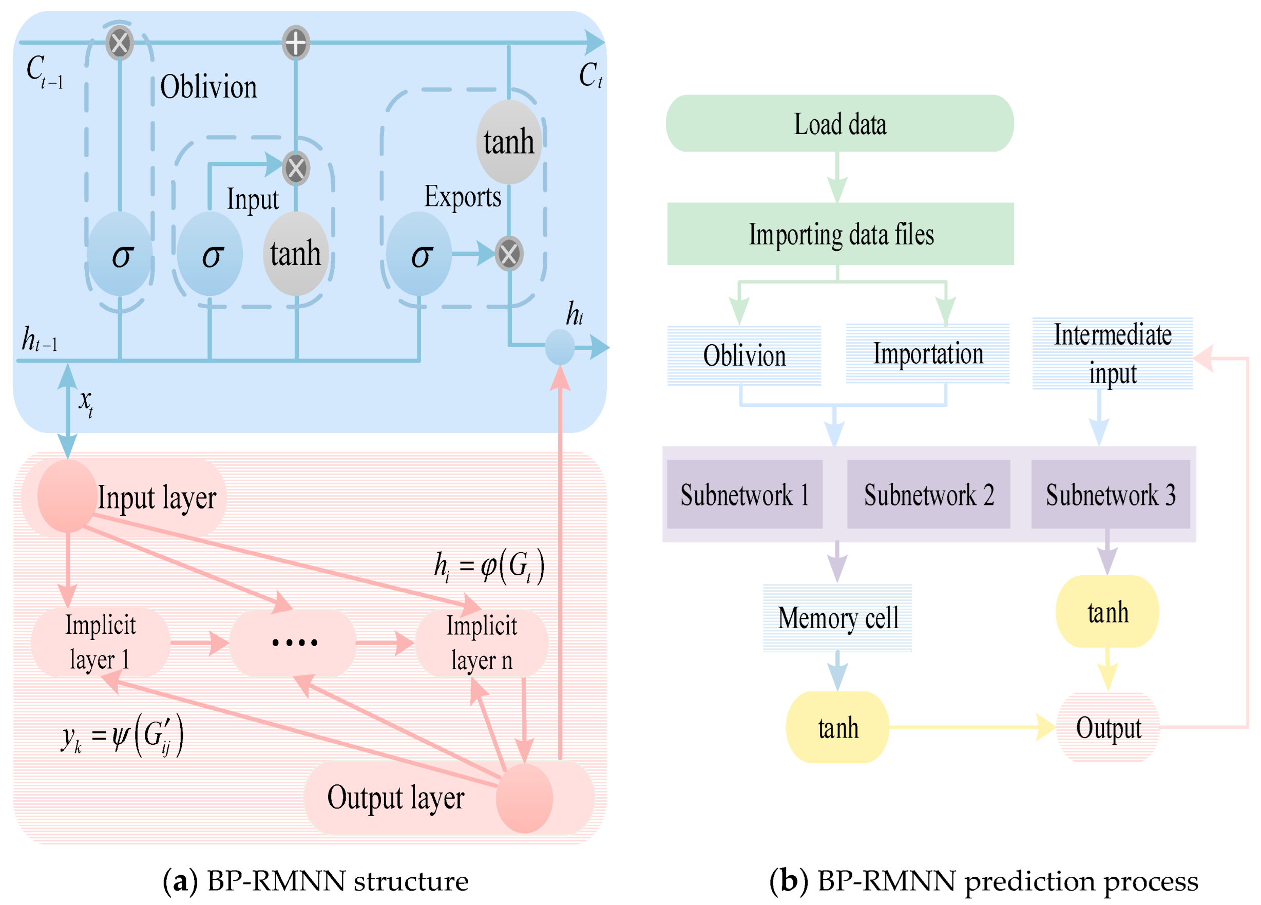
This paper analyzes the parameter optimization and model structure of the prediction model. For parameter optimization, evolutionary algorithms have been widely used by scholars. However, an evolutionary search requires a complete search space. For example, the particle swarm mimics the process of birds foraging in the forest, and the ant colony mimics the process of ants on the ground. Genetic algorithms refer to chromosomal crossover and mutation in human genetics, encoding parameters into chromosomes for evolution; however, these algorithms need to use binary coding calculations, and the sequence length and space are difficult to meet the requirements. Quantum genetics theory originates from the concept of quantum computing proposed by Feynman, an American physicist. With the development of the quantum field, more and more scholars use the superposition, entanglement, and convergence characteristics of quantum mechanics to increase the superposition state between 0 and 1, thereby increasing the search space and further improving the accuracy of the model. As for the model structure problem, the classical LSTM structure will cause the problem of increased operation cost and low prediction accuracy in environments with more hyperparameters. As a mature optimization method, the artificial neural network has the advantages of a simple structure, low cost, and strong plasticity; therefore, this paper uses an artificial neural network combined with the incentive function module of the LSTM network. The core memory unit, input unit, and output unit are optimized using a better search algorithm.

This study introduces a short-term power load forecasting method. It employs a quantum genetic algorithm (QGA) to enhance a recurrent memory neural network (RMNN). The goal is to integrate traditional algorithms with advanced techniques, creating an improved model. This method increases the result accuracy and reliability. The RMNN we developed includes memory, input, and output units derived from an LSTM network. Consequently, the model can recognize time-based patterns and complex features in power load data. The LSTM memory unit utilizes gates—input, forget, and output gates—to address common issues like gradient vanishing and explosion. These issues frequently arise in standard RNNs with lengthy data sequences. The gates help the model perform better with long-term patterns.

To make the RMNN work better, we use the QGA to adjust its hyperparameters. The QGA mixes quantum computing with genetic algorithms. It uses quantum bits and quantum rotation gates to search the whole solution space and find the best results. Compared to regular genetic algorithms, the QGA searches more thoroughly and converges faster. This makes it very good for complex, high-dimensional problems.

This paper tests the new method against other forecasting models. We use real power load data from a regional system. The QGA-RMNN model works better than support vector machine (SVM) and regular LSTM networks. It is more accurate, faster, and more stable. The model obtains good results. It greatly reduces the MAPE error. It also greatly improves the MAE error.

Regarding the structure of the paper, the introduction first analyzes the research progress in electric load forecasting and clarifies the optimization direction of this study. Section 2 elaborates on the theory of the quantum genetic algorithm (QGA) and explains the quantum adaptive rotation optimization strategy. Section 3 constructs a recurrent memory neural network structure based on artificial neural networks and long- and short-term memory (LSTM) networks. Section 4 describes the mechanism and process of optimizing the hyperparameters of the recurrent memory network using the QGA. Section 5 validates the adaptability and accuracy of the proposed prediction model through two electric load forecasting case studies.

2. Quantum Genetic Foundations

2.1. Quantum Computing Theory

The quantum genetic algorithm (QGA) is an advanced evolutionary algorithm based on the principles of quantum mechanics. It uses quantum superposition states and quantum crossover operations to create “intermediate states,” which help increase population diversity. Studies show that the QGA, because of its unique evolutionary methods and design, is good at solving complex optimization problems. Recently, the QGA has made great progress in areas like parameter optimization, numerical prediction, and artificial intelligence, gaining attention from researchers. The QGA works well with high-dimensional and nonlinear problems, offering better global search abilities and faster convergence, which helps solve tough engineering challenges [19,20,21].

The combination of quantum genetic algorithms with optimization methods has greatly improved global search ability and convergence speed. Adding quantum behavior to the squirrel search algorithm (SSA) through quantum state-dependent position updates helps solve the problem of premature convergence in standard SSA models [22]. Also, the hybrid quantum–classical system that pairs QGA with quantum gate circuit neural networks (QGCNNs) shows better parallel computing power. This new design is especially good at solving complex optimization problems with uncertainty and ambiguity [23]. These advances show that the QGA is very effective at global optimization and fast searching, making it a strong tool for demanding optimization tasks.

2.2. Quantum Genetic Optimization Algorithm

Classical genetic algorithms update parameters by evolving them through crossover and coding to find better solutions in the probabilistic search space. However, classical genetic algorithms (GAs), which use binary-encoded chromosomes, have limitations when dealing with large datasets and high-dimensional variables. Binary chromosome encoding in GAs is fast and easy to implement, but it encounters challenges when solving high-dimensional and large-scale optimization tasks [24]. Studies show that binary encoding can lead to very-long gene sequences, expanding the search space significantly when handling complex tasks with many variables and large datasets, thereby reducing the algorithm’s performance [25]. However, the quantum genetic algorithm (QGA) significantly enhances search speed and efficiency through quantum encoding and quantum rotation. When dealing with high-dimensional datasets featuring numerous variables, the QGA demonstrates a clear advantage. This is attributed to its ability to explore multiple solutions simultaneously via quantum superposition and entanglement, enabling it to cover a large search space more effectively and avoid local optima. Additionally, the use of quantum gates for operations such as mutation and crossover further optimizes the search process. The qubit-based encoding method increases population diversity, which aids in finding the best solutions. Furthermore, refining how quantum bits converge is essential to improving the chances of finding the best solution.

(1)

Quantum Feature

The essential difference between quantum and classical computation stems from their distinct state representations. While classical computation is restricted to binary digits (0 and 1), quantum computation exploits the principles of superposition, quantum coherence, and entanglement to create qubit states that simultaneously occupy a continuum between the classical states.

(2)

Quantum Unit

The fundamental unit in quantum states is the quantum bit (qubit) $\left|\psi 〉\right.$, which encompasses both ground states and superposition states. The relationship between different quantum states can be mathematically represented using probability amplitudes $\alpha$ and $\beta$, denoted as $\left|\psi 〉\right.=\alpha \left|0〉+\beta \right.\left|1〉\right.$. The correlation between the superposition state $\left|\psi 〉\right.$ and the ground state x can be expressed as follows:

$$\left|\psi 〉\right.={\displaystyle \sum _{x\in {(0,1)}^n}{\alpha }_x}\left.\left|x〉\right.\right|{{\displaystyle \sum _{x\in {(0,1)}^n}\left|{\alpha }_x\right|}}^2=1$$

(1)

Equation (1) can be expressed in matrix form. In quantum computing systems, the quantum bit (qubit), which is the fundamental information unit of quantum states, can be mathematically characterized as follows: For multi-qubit systems, the quantum state is formed through the tensor product superposition of single-qubit states. Specifically, the probability of the ith qubit being in the ground state |0⟩, as determined using the squared modulus of its probability amplitude (i.e., the observation probability), is given by the square of the absolute value of the corresponding quantum state coefficient. Furthermore, the post-measurement state collapses to the following:

$$\left|{\psi }_x〉\right.={\displaystyle \frac{{\alpha }_{\left.1\right|y_i=0}\left|x_1〉+\right.{\alpha }_{\left.2\right|y_i=0}\left|x_2〉+\cdots +\right.{\alpha }_{\left.2^N\right|y_i=0}\left|x_{2^N}〉\right.}{\sqrt{{\left|{\alpha }_1\right|}^2+{\left|{\alpha }_2\right|}^2+\cdots +{\left|{\alpha }_{2^N}\right|}^2}}}$$

(2)

(3)

Quantum Rotation

The quantum rotation operator is denoted as R, which represents a unitary transformation in Hilbert space. To satisfy the normalization condition requiring the sum of squared probability amplitudes to equal unity, the probability amplitudes can be geometrically represented on a unit circle. The corresponding rotation matrix is given as follows:

$$\left|{\psi }^{\prime }〉\right.=R(\theta )\times \left|\psi 〉\right.=\left[\begin{array}{cc}\cos \theta & -\sin \theta \\ \sin \theta & \cos \theta \end{array}\right]\left[\begin{array}{c}\alpha \\ \beta \end{array}\right]=\left[\begin{array}{c}{\alpha }^{\prime }\\ {\beta }^{\prime }\end{array}\right]$$

(3)

In Equation (3), $R(\theta )$ represents the angular rotation function, $\theta$ denotes the rotation angle, and ${\theta }_{\max }(m)$ corresponds to the rotational step size.

(4)

Quantum Encoding

The probability amplitudes associated with quantum bits (qubits) can represent a collection of qubit pairs, facilitating the observation of quantum transitions from superposition states to ground states. Within an N-qubit quantum system, the qubit pair located at the nth position can be mathematically represented as $q_n=\left[\begin{array}{ll}{\alpha }_n& {\beta }_n\end{array}\right]|{\alpha }_x^2+{\beta }_x^2=1$.

(5)

Quantum Evolution

① The genes of individuals undergo modifications in their probability amplitudes via crossover and mutation operations, resulting in a variety of quantum superposition states. The ensemble of these quantum superposition states constitutes the population Q(m). In this context, m represents the count of evolutionary iterations, and everyone in the population is denoted as $q_i^m$, where i corresponds to the ith individual within the population. An individual consists of n qubit pairs, and the probability amplitudes associated with the chromosomes at the inception of the evolutionary process are specified as $\left|{\alpha }_x\right|=\left|{\beta }_x\right|=1/\sqrt{2}$.

② After m iterations of population evolution, a set of solutions is created, and their fitness is checked using a fitness function f(m). In traditional quantum genetic algorithms, fitness values are directly included in the solution space. This leads to the probability of amplitude space for individuals being limited to the areas affected by the rotation matrix, often causing early convergence and lower fitness performance.

③ To optimize rotation, the population size must be increased while also reducing the computational load. To solve this, a sparsity factor is added to the rotation process, which creates a non-uniform distribution of rotation angles (probability amplitudes). Based on the sparse factor, the search space for the hyperparameter optimization of the QGA can be significantly expanded, thereby enabling the rapid attainment of more optimal values. This method increases the density of rotation angles in areas with higher fitness, which improves optimization efficiency. The rotation angle strategy factor is expressed as follows:

$$\left|{\psi }^{\prime }〉\right.=R({\theta }^{\prime }(m))\times \left|\psi 〉\right.=\left[\begin{array}{cc}\cos {\theta }^{\prime }(m)& -\sin {\theta }^{\prime }(m)\\ \sin {\theta }^{\prime }(m)& \cos {\theta }^{\prime }(m)\end{array}\right]\left[\begin{array}{c}\alpha \\ \beta \end{array}\right]=\left[\begin{array}{c}{\alpha }^{\prime }\\ {\beta }^{\prime }\end{array}\right]$$

(4)

The rotation angle function in Equation (4) is given as follows:

$${\theta }^{\prime }\left(m\right)={\theta }_{\max }\left(m\right)-{\displaystyle \frac{f\left(m_i\right)-f\left(m_{\max }\right)}{f\left(m_{\max }\right)}}\cdot {\theta }_{\max }^{\prime }\left(m\right)$$

(5)

In this case, the classical quantum rotation angle is shown as ${\theta }_{\max }\left(m\right)$, and the fitness function value at the search location is given by $f\left(m_i\right)$. As shown in Equation (5), the optimized quantum rotation angle changes by lowering the step size in high-fitness areas and increasing it in low-fitness areas. This method allows us to search for the best solution without increasing computational cost.

This study now looks at how the QGA can be used to optimize parameters in artificial recurrent memory networks to improve short-term load forecasting accuracy. Artificial recurrent networks are good for processing sequential data, but their performance depends on how the parameters are set. Traditional optimization methods often fail when dealing with high-dimensional and nonlinear parameter spaces. The QGA, which combines the parallel power of quantum computing with the global search abilities of genetic algorithms, offers a new solution to this problem. The paper will now look at the design of artificial recurrent memory networks and how they can be used in short-term load prediction.

3. Artificial Recurrent Memory Networks

3.1. Artificial Recurrent Neural Network Model

Artificial recurrent networks, which derive from BP neural networks, create a node-weight transmission network. This algorithm is widely utilized in machine learning and pattern recognition [26]. Its main advantages include its simple network structure and efficient weight adjustment method. The weights are adjusted through the error backpropagation algorithm, which optimizes the connections between the input and output layers [27]. However, these networks can encounter premature convergence. Consequently, researchers have begun to combine the classical BP neural network with other optimization algorithms to minimize these errors.

The BP network is structured into three key layers—the first layer is the input layer, the second layer is the hidden layer, and the third layer is the output layer. For a classical BP network, the mathematical expressions governing the input and output are formulated as follows:

$$\begin{array}{c}{y}_k=\psi (W_{jk}^{″}\cdot \phi ({\displaystyle \sum _{i=1}^n}{W}_{ij}^{\prime }\cdot x_i^{\prime }+b_i^{\prime })+b_j^{″})\\ =\psi \left(G^{″}(W_{jk}^{″}\cdot \phi \left(G^{\prime }\right)+b_j^{″})\right)\end{array}$$

(6)

Leveraging the strong nonlinearity and high adaptability of BP neural networks, this paper introduces a recurrent search module into the classical BP network and divides the network into several sub-networks $G_t$, each of which has multiple inputs but only one output. The output of a sub-network is computed based on multiple inputs, weights, and biases, as described by the following equation: $G_t=W_t{x}_t+b_t$. In the given equation, W corresponds to the weight matrix, x is the input column matrix, and b represents the bias column matrix. The outputs of multiple sub-networks within the input layer space are fed as inputs to the subsequent layer (hidden layer), ultimately propagating to the output layer. The recurrent search module is implemented to assess the reliability of the output values at each layer, and an adaptive function P is formulated as follows:

$$P=\frac{|y_k^{\prime }-y_k|}{y_k}\times 100\%$$

(7)

The role of the adaptive function is to enhance the training speed of the model. By dynamically adjusting the parameters of the recurrent module based on the adaptive function, the network parameters that meet the model’s requirements can be obtained, thereby improving the model’s performance or the stability of the system. Artificial recurrent neural networks iteratively explore the number of hidden layers and the number of nodes in each hidden layer, while the number of input and output nodes remains fixed. The structural configuration of the network is shown in Figure 1.

3.2. Long- and Short-Term Memory Prediction Models

LSTM networks constitute an advanced variant of recurrent neural networks (RNNs), where the cell state plays a pivotal role by traversing the entire network to facilitate stable information propagation across sequential time steps. The LSTM network controls the flow of information to obtain long-term dependencies and mitigates the challenges of gradient vanishing and short-term memory that are inherent in conventional RNNs [28,29]. The fundamental innovation of LSTM networks resides in their distinctive memory cell structure, which facilitates the selective retention or elimination of information, thereby enabling the robust modeling of long-term dependencies in sequential data. Empirical studies have shown that LSTM achieves exceptional performance in handling time series data characterized by strong regularity, such as in stock price forecasting and weather prediction, where its predictive accuracy markedly surpasses that of conventional RNN models [30].

The transmission state of the LSTM core memory unit includes input, computation, control, forget, and output operations. The memory unit decides whether to discard or retain information or data from the preceding unit. Intermediate input data $x_t$ and intermediate output data $h_{t-1}$ from the previous unit are concurrently input into the input unit. The $\sigma$ and Sigmoid functions are employed to generate the information to be memorized $o_t$. This memorized information $o_t$ is then processed by the output unit to produce intermediate outputs $h_t$. The formulas for the memory unit, input unit, and output unit are shown in

Table 1. LSTM core unit calculation formulas.

Core Control Unit	Formula
Memory unit	$f_t=\sigma (W_{f_1}\cdot x_t+W_{f_2}\cdot h_{t-1}+b_f)$
Input unit	$i_t=\sigma (W_{i_1}\cdot x_t+W_{i_2}\cdot h_{t-1}+b_i)$
Output unit	$o_t=\sigma (W_{o_1}\cdot x_t+W_{o_2}\cdot h_{t-1}+b_o)$
Intermediate input unit	$g_t=\tanh (W_{g_1}\cdot x_t+W_{g_2}\cdot h_{t-1}+b_g)$
Cell state unit	$C_t=g_t\otimes i_t+C_{t-1}\otimes f_t$
Intermediate output unit	$h_t=\tanh (S_t)\otimes o_i$

.

Figure 2 demonstrates that the LSTM network incorporates many computational units, including the count of hidden layers Net₁ and the associated memory units per hidden layer Net₂. This leads to considerable computational expenses and instances of premature convergence. In response, the literature utilizes an exhaustive search approach to derive optimized configurations, though this further escalates computational demands.

In scenarios where the combination space is extensive and the complexity is elevated, traditional search algorithms prove insufficient. To address this, the complex structure must be either aggregated or partitioned, and the inputs and outputs of the LSTM are modeled via sub-networks $G_t$ as follows:

$$\begin{array}{l}{S}_t=\tanh \left(G_{gxt}+G_{gh(t-1)}\right)\otimes \sigma \left(G_{ixt}+G_{ih(t-1)}\right)+b_{it}\\ \begin{array}{cc}& =S_{t-1}\end{array}\otimes \sigma \left(G_{fxt}+G_{fh(t-1)}\right)+b_{it}\end{array}$$

(8)

Utilizing Equation (8), the artificial recurrent network is fused with the components of the LSTM network, and the prediction speed and accuracy are further improved by modifying the number of memory nodes and hidden layers, thereby obtaining a recurrent memory neural network (RMNN) model with a higher prediction accuracy. The architecture of the optimized recurrent memory network and its prediction process are depicted in Figure 2a,b.

4. QGA-RMNN-Based Predictive Models

In this paper, the key node parameters of the artificial recurrent memory network are optimized through the QGA. The QGA-RMNN model is then applied to forecast the load on the test dataset. To overcome the shortcomings of conventional prediction approaches, the load data undergo normalization analysis, with data correction and numerical interpolation applied to accentuate its cyclic sequences. Following this, the artificial recurrent network is trained, and the QGA adjusts the number of nodes in the hidden layer and the weights of the connections between layers. The deviation function serves as the fitness function, and the optimization trajectory of the QGA-RMNN prediction model is depicted in Figure 3.

During the data preparation phase, the load data serve as the input for the forecasting model and act fundamentally as a time series. To ensure data quality and integrity, a preliminary inspection of the load data is conducted. Missing values and zero entries can be addressed with interpolation techniques such as linear interpolation or spline interpolation. Additionally, outliers or excessively large values can be managed through normalization or truncation methods to improve data consistency and enhance model performance. In the BP-RMNN, the input layer receives preprocessed data, while the hidden layer consists of multiple neurons that utilize the tanh activation function to introduce nonlinearity. The output layer generates the model’s prediction results. To enhance forecasting performance, an optimization algorithm is employed to adaptively search for the global optimum by adjusting the model parameters through rotational angle optimization.

During the training process, the number of training iterations is initially determined, and the LSTM model is refined from both structural and parametric perspectives. The key hyperparameters include the number of iterations (N₁), initial train rate, train rate drop period, and learning rate decay factor. The initial train rate determines the step size for updating model parameters, while the train rate drop period gradually reduces the learning rate as training progresses to enhance convergence stability. The learning rate decay factor specifies the proportion by which the learning rate decreases at each update step, ensuring a balanced trade-off between convergence speed and model performance. The search range for the iteration count parameter of the RMNN is from 1500 to 3000, with an interval of 10. The search range for the initial training rate parameter is from 0.0005 to 0.015, with an interval of 0.0005. The search space for the training rate drop period parameter is from 500 to 1500, with an interval of 10. The search range for the learning rate decay factor parameter is from 0.05 to 0.5, with an interval of 0.05. The deviation function used in the search process is the residual sum of squares (RSS).

Compared with other combined optimization prediction models, in terms of structure, the QGA-RMNN employs quantum optimization and a recurrent memory structure, which gives it an advantage over traditional search–prediction combined models in terms of search performance and adaptability. In terms of computation, the prediction model has certain advantages in training time, adaptability, and prediction accuracy. Compared with the CNN-LSTM and GA-BPNN combined models, under the same accuracy requirements, the training time of the QGA-RMNN is less than that of the CNN-LSTM model, with the training and prediction time of the latter being within 50 s, while the training time of the CNN-LSTM model is over 100 s. Compared with the MLS-SVM and GA-LSTM combined models, the QGA-RMNN has a shorter training time and a higher accuracy.

5. Case Study Validation

To assess the adaptability and accuracy of the short-term load forecasting model introduced in this study across various settings, we selected electricity load data from two distinct regions, each with unique characteristics. Specifically, we utilized load data from a microgrid and the Elia grid in Belgium.

The microgrid data reflect the localized electricity consumption patterns typical of small-scale power systems, primarily driven by the operational activities within the area it serves. In contrast, the Elia grid data capture the electricity consumption patterns of a large-scale, regional power system, influenced by diverse factors such as weather, economic activities, and social behaviors.

Validating the model with these two datasets demonstrates its capacity to manage diverse load patterns and operational conditions. The model’s performance in predicting short-term load variations in the microgrid setting highlights its precision in localized contexts. Meanwhile, its ability to handle the more complex load patterns of the Elia grid underscores its robustness. This dual validation not only enhances the model’s reliability but also confirms its broad applicability across different environments.

5.1. QGA and RMNN Parametric Analysis

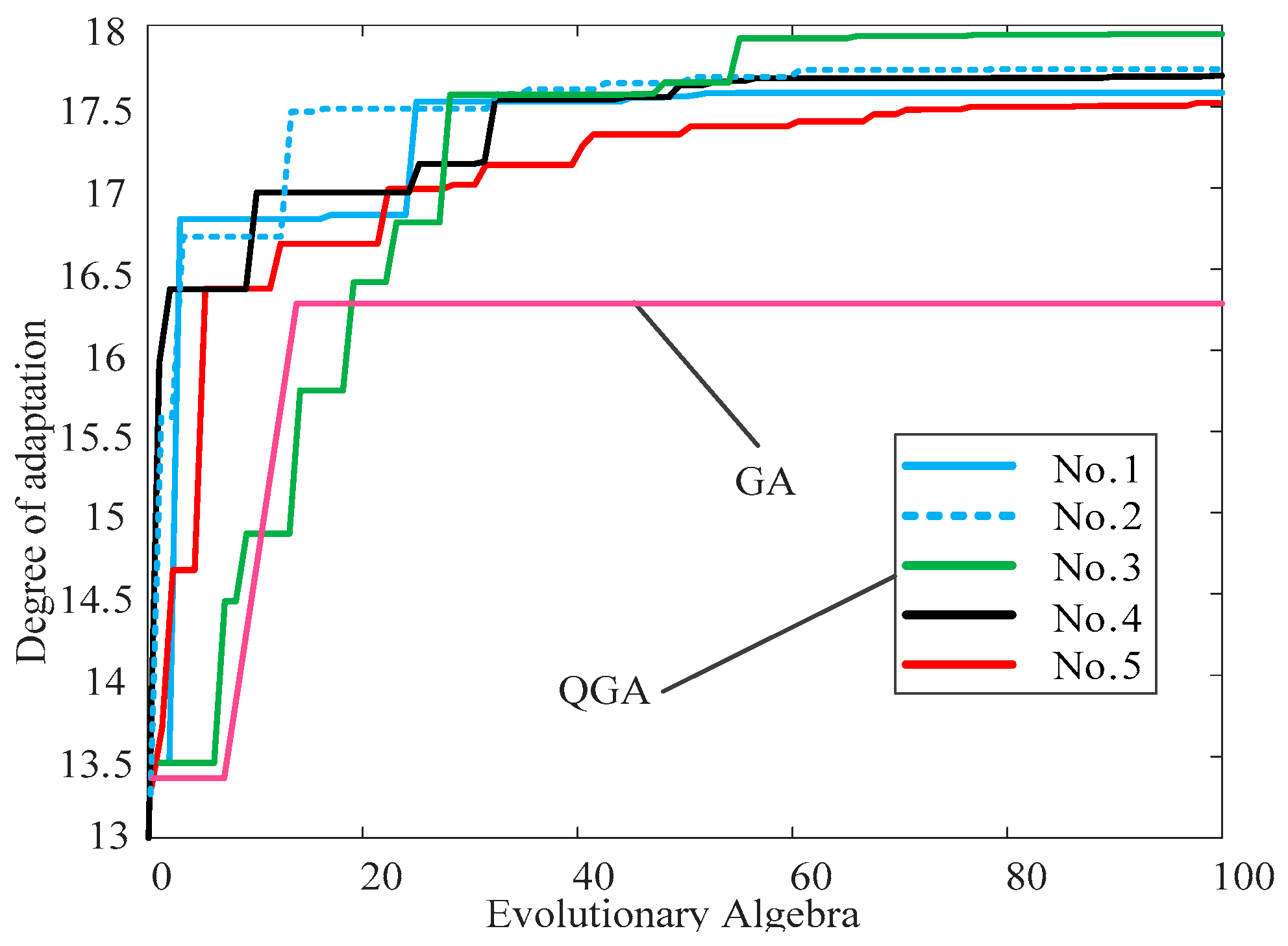
To verify the advantages of the QGA in search performance, five sets of training data were used for validation. Among them, sparse factors were added to the first four sets, while the fifth set did not contain sparse factors. The outcomes of these experiments are depicted in Figure 4. As can be seen from the figure, the fitness of the QGA is significantly higher than that of the traditional genetic algorithm (GA). On the other hand, the LSTM module is optimized in terms of both its architecture and parameters. Parametric optimization encompasses the iteration count N1, the initial train rate, the train rate drop period, and the learning rate decay factor. Among them, the iteration count is 2000, the initial training rate is 0.005, the training rate drop period is 800, and the learning rate decay factor is 0.1.

During the testing phase, the MAPE and RMSE are employed as fitness output measures. The mathematical formulations for these metrics are provided below.

$$MAPE={\displaystyle \frac{1}{n}}{\displaystyle \sum _{i=1}^n\left|\frac{Z_{ip}-Z_{it}}{Z_{it}}\right|\times 100}\%$$

(9)

$$RMSE=\sqrt{{\displaystyle \frac{1}{n}}{\displaystyle \sum _{i=1}^n{\left(Z_{ip}-Z_{it}\right)}^2}}$$

(10)

In Equations (6) and (7), $Z_{ip}$ represents the forecasted value, while $Z_{it}$ indicates the true value.

5.2. Case Study 1

The dataset for Case Study 1 originates from the load parameters of a microgrid. Sampling is performed at 15 min intervals, yielding 96 daily sampling points. By utilizing the time associated with each sampling point as a dimension, the daily data are converted into a 96-dimensional input load matrix, with the date acting as the time series value. In this study, the load data from December 2nd to December 10th in Region A were employed as the training dataset, resulting in a time series length of 9 for each training dimension. The initial sliding window on December 11th was utilized as the validation set, whereas the remaining data were allocated to the test set. The prediction process utilizes a sliding window approach, with key parameters including the sliding window dimension and span. Given the limited number of parameters involved in the sliding window approach and the relative ease of obtaining their optimal values, the study employs an empirical method to determine these values. Specifically, based on a single RMNN model, the sliding window dimension range is set between 10 and 25, while the span range is set between 3 and 9. Various combinations of these parameters are tested to identify the optimal configuration. The results indicate that a sliding window dimension of 15 and a step size of 6 provide superior prediction performance. In other words, the optimal sliding window configuration is a dimension of 15 (equivalent to 225 min) with a step size of 6 (90 min).

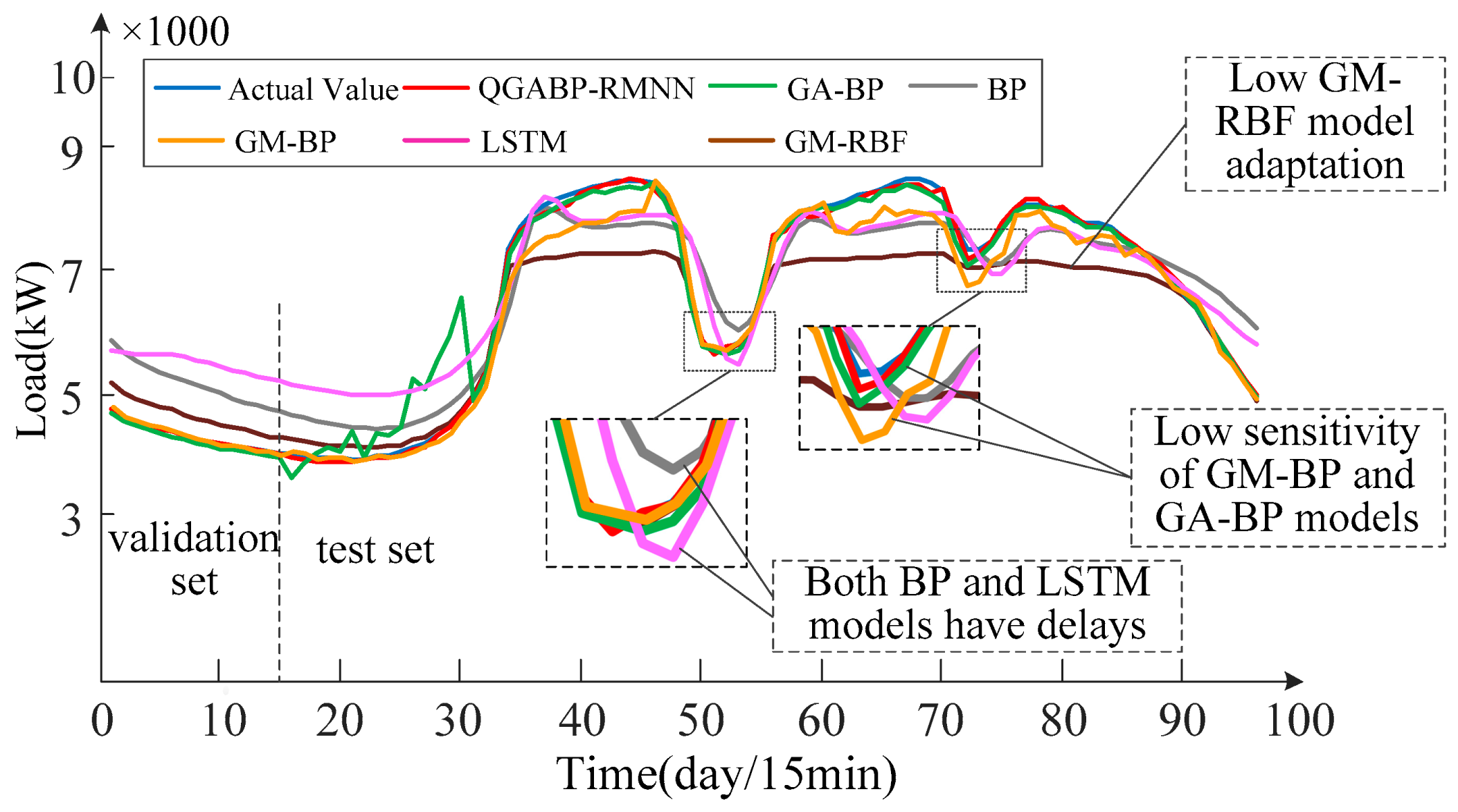
The load forecasting performance of the QGA-RMNN method is illustrated in Figure 5. To demonstrate the innovation and value of the proposed model, as well as to validate the optimization effects of quantum genetic algorithms and artificial intelligence, this study compares the proposed QGA-RMNN model with five other models—the BP network model optimized by genetic algorithm (GA-BP) [31], the classical LSTM model, the BP network model based on gray theory (GM-BP) [32,33], the BP network model optimized by genetic algorithm [34], and the hybrid model based on Gaussian mixture model and radial basis function (GM-RBF) [35]. The evaluation of these algorithms’ predictive capabilities is carried out through technical indicators.

Figure 5 shows the forecast performance of different models. The QGA-RMNN model performs much better than the others in terms of prediction accuracy.

First, the forecasting curve of the QGA-RMNN is closest to the actual load values, especially during times of big load changes, like between the 30th and 50th days. This shows that the QGA-RMNN is more accurate and better at handling load changes.

Second, compared to other models, the QGA-RMNN is more stable in both the validation and test sets. For example, the LSTM model has large prediction errors at certain times, while the GA-BP and GM-BP models show a lower accuracy during sudden load changes. In contrast, the QGA-RMNN stays accurate throughout the forecasting period, showing that it handles complex load changes better.

Also, the deviation values are much higher at the peak and valley points. The LSTM model shows less accuracy at peak points and has a delay effect. The GM-BP model combines good short-term accuracy with the adaptive nature of BP networks in the medium-to-long term. But when the sample size is small and the BP network’s values are not enough, large errors can occur. The GM-RBF model has low computation costs, a simple structure, and fast speeds, but it struggles to predict deviations and fluctuating regions. On the other hand, the QGA-RMNN, which uses parameter optimization with quantum genetic algorithms and sliding window strategies, has a better accuracy than the other models in these regions.

When comparing LSTM optimization, the recurrent memory network shows that the LSTM model has a delay effect and big errors at peak points. The LSTM model, optimized with quantum genetic algorithms and artificial recurrent techniques, does much better than the basic LSTM model, with an average deviation of only 0.55%. It also gives much better predictions for load time series with clear patterns and volatility.

Table 2. Comparison of the prediction effect of the QGA-RMNN model and the LSTM model.

	Index	Time(s)	RMSE	MAE	MAPE (%)
Prediction Algorithm
QGA-RMNN		<50	53.8516	39.8025	0.5551
LSTM		<25	581.606	475.678	7.4079
GA-BPNN		<200	283.183	192.163	2.4288
GM-BPNN		Long	505.889	326.122	5.6176
GA-RBF		<10	518.091	452.523	6.5423
MLS-SVM		<100	369.300	229.500	3.4500

compares the MAPE, MAE, and RMSE metrics of the prediction methods used in several referenced studies and the method proposed here. The proposed method shows a better prediction accuracy than the GA-RBF, GM-BP, and LSTM methods.

Also, in terms of computational time, the proposed method not only improves prediction accuracy but also performs better in computational cost, sequence length selection, and spatial robustness compared to the MLS-SVM and GA-BP algorithms. This multi-dimensional improvement moves traditional predictive modeling forward.

The experimental results show that the proposed method works better in terms of both prediction accuracy and stability across different scenarios. These results show the algorithm’s strength and ability to adapt, showing its potential to solve complex real-world problems. The improvements in accuracy and stability confirm the effectiveness of the proposed method, opening up new possibilities for research and practical use in this field.

5.3. Case Study 2

The data for Case Study 2 come from the Elia grid load in Belgium, Europe. The sampling interval is 15 min, resulting in 96 load sampling points per day. The daily data are transformed into a 96-dimensional input load matrix. The time for each sampling point is used as a dimension. Central European Time (CET) is applied as the time series value. The training set has a sequence length of 192, while the testing set has a length of 96. A sliding window strategy with a dimension of 15 (equivalent to 225 min) is used during the prediction phase. The prediction accuracy for the training and testing sets is shown in Figure 6 and Figure 7, respectively.

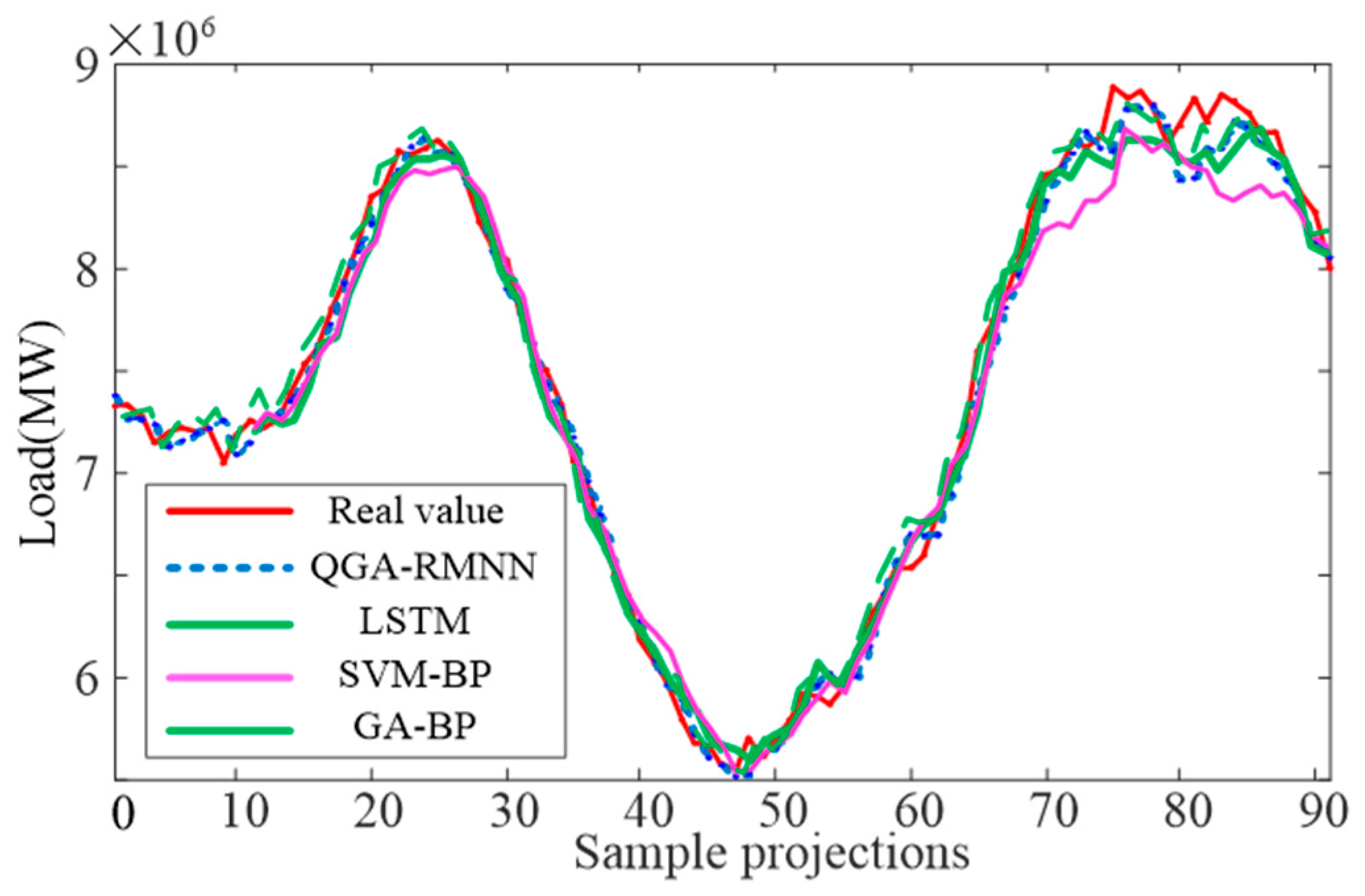
To show the advantages of the proposed model, we compare the QGA-RMNN model with several high-precision models from Case Study 1. These models include the GA-BP model, the LSTM model, and the SVM-BP model. We assess their predictive capabilities using RMSE as the evaluation benchmark.

Analysis of the training set shows that the proposed model captures power load variations with great precision. There are slight deviations in areas with high variability, but the model performs exceptionally well in stable regions. Deviations at peak and trough points stay below 2%, with a total deviation of 1.03%. This confirms the reliability of the training set.

For the test set, the prediction results show that the peak load duration is longer in later peak regions. The load values are also higher in these areas. This causes a reduction in accuracy across all models. The SVM-BP model shows the largest decline. It has a deviation of 4.9% at the second peak.

The other three models perform similarly. They maintain peak position deviations within 2%. The LSTM model shows higher volatility during smooth load increases. The GA-BP model has a lower accuracy during the early stages of load growth. These models have deviations of 1.45% and 1.33%, respectively. Both are higher than the 1.01% deviation of the proposed model.

Overall, the QGA-RMNN model demonstrates a superior predictive performance.

The predictive precision of the QGA-RMNN model is depicted in Figure 8. From the perspective of computational cost, the SVM-BP model has the lowest training cost but suffers from a lower accuracy, while the other three models exhibit similar training times. By analyzing Figure 6, Figure 7 and Figure 8, it can be observed that the RMSE of the QGA-RMNN model is only 101,748, whereas the RMSE values for the LSTM, SVM-BP, and GA-BP models are 134,049, 148,128, and 127,245, respectively. The empirical outcomes reveal that the QGA-RMNN model substantially outperforms other algorithms in terms of prediction accuracy.

Table 3. Comparison of the prediction effect of models in Case Study 2.

	Index	Time(s)	RMSE	MAE	MAPE (%)
Prediction Algorithm
QGA-RMNN		<50	101,748	82,712.88	1.01
LSTM		<25	134,049	10,897.97	1.45
GA-BPNN		<200	127,245	97,376.36	1.33
SVM-BP		<100	148,128	112,891.22	1.67

compares different prediction methods from existing studies and the proposed method for Case Study 2, using three key metrics—MAPE, MAE, and RMSE. The results show that the proposed method has a better prediction accuracy than the LSTM approach.

Also, compared to the SVM-BP and GA-BP algorithms, the proposed model not only gives a higher prediction accuracy but also performs better in terms of computational cost, sequence length selection, and spatial robustness. By improving multiple areas, the proposed method makes the traditional predictive modeling framework more efficient and reliable.

In Case Study 2, the effectiveness and flexibility of the proposed method were confirmed through data analysis and comparisons with several traditional models. The results show that the proposed method always performs better in terms of prediction accuracy and is more adaptable and robust in handling complex nonlinear relationships. A closer look at key performance metrics shows that the method can find hidden data patterns and dynamic features. These results support the findings of Case Study 1 and expand the method’s potential use, providing a stronger foundation for its use in real-world engineering.

6. Conclusions

This paper presents a short-term power load forecasting method using a quantum genetic algorithm (QGA) to optimize an artificial recurrent neural network (RMNN). Experimental results show that the QGA has strong benefits in optimizing RMNN parameters, solving the local optima problem found in traditional methods. It improves the search space for parameter nodes in forecasting models based on artificial intelligence, making the predictions more global and efficient. Compared to existing models, the proposed method gives better accuracy and stability on multiple publicly available datasets. At the same time, recurrent memory networks can combine the strengths of both traditional and advanced algorithms. By using combinations of artificial networks to optimize the memory, input, and output units of the LSTM network, and using the QGA to optimize the parameters, the LSTM network is further improved. Also, parallel computation lowers the computational cost, speeding up the model and making it more adaptable. This approach gives new reference points for accurate forecasting tasks.

The forecasting model in this study not only offers valuable reference and practical use for short-term electricity load forecasting but also has the potential for use in other predictive tasks in the power system field, such as wind power grid forecasting and energy usage prediction. Since CNNs are good at handling high-dimensional data and capturing complex patterns, the next step will be to explore using CNNs and Random Forests to extract key features related to electricity load. This method is expected to improve the accuracy of the parallel group optimization-based load forecasting method.