Abstract
To facilitate power system decarbonization, optimizing clean energy integration has emerged as a critical pathway for establishing sustainable power infrastructure. This study addresses the multi-timescale operational challenges inherent in power networks with high renewable penetration, proposing a novel stochastic dynamic programming framework that synergizes intraday microgrid dispatch with a multi-phase carbon cost calculation mechanism. A probabilistic carbon flux quantification model is developed, incorporating source–load carbon flow tracing and nonconvex carbon pricing dynamics to enhance environmental–economic co-optimization constraints. The spatiotemporally coupled multi-microgrid (MMG) coordination paradigm is reformulated as a continuous state-action Markov game process governed by stochastic differential Stackelberg game principles. A communication mechanism-enabled multi-agent twin-delayed deep deterministic policy gradient (CMMA-TD3) algorithm is implemented to achieve Pareto-optimal solutions through cyber–physical collaboration. Results of the measurements in the MMG containing three microgrids show that the proposed approach reduces operation costs by 61.59% and carbon emissions by 27.95% compared to the least effective benchmark solution.
1. Introduction
Driven by sustained global economic growth and technological advancement, global fossil energy consumption has exhibited an exponential growth trajectory. Greenhouse gases from fossil energy combustion contribute to global warming and the frequency of extreme weather events. To address this planetary-scale challenge, the international community is accelerating energy transition initiatives, with the large-scale deployment of renewable energy, primarily wind turbine (WT) and photovoltaic (PV) systems, positioned as the cornerstone strategy for achieving carbon neutrality objectives [,].
China introduced its dual carbon goals of achieving carbon peaking by 2030 and carbon neutrality by 2060 in 2021, aiming to accelerate the transition of its power system by prioritizing renewable energy deployment (e.g., WT and PV) to reduce fossil fuel dependency []. However, the inherent variability and intermittency of renewable energy sources have hindered their effective integration into the microgrid (MG) that integrates distributed power sources, energy storage devices, and loads, limiting capacity expansion. A significant penetration of renewable energy into the microgrid may lead to challenges such as abrupt voltage fluctuations [,]. This necessitates innovative energy management strategies that reconcile rising consumption with decarbonization imperatives. Within the power sector, fossil-based generation continues to account for the largest share of electricity production, inevitably generating CO2 emissions during operation []. The electricity generation percentage of China and worldwide from various energy sources in 2024 is shown in Figure 1. Given the direct linkage between power generation and carbon footprints, extensive research has focused on optimizing emission reduction pathways from the supply side, including carbon capture retrofitting, fuel-switching technologies, and efficiency-driven dispatch models.
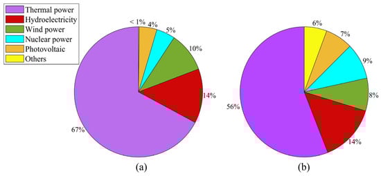
Figure 1.
The electricity generation percentage of China and worldwide from various energy sources. (a) China; (b) worldwide.
Recent research demonstrates that advanced multi-energy conversion technologies, including micro-combined heat and power systems and electrically driven heat pumps, enable systemic energy efficiency enhancements and decarbonization through synergistic integration with multiple energy vectors (electrical, thermal, and cooling) []. In particular, the ability to regulate the dynamics of carbon flows, as a key medium linking energy conversion and carbon emissions, directly affects the level of decarbonized operation of the system. A blank planning model for energy–carbon coupled multi-energy flow synergistic optimization is established to implement system-wide collaborative design under the constraints of multi-energy–carbon flow []. In order to enhance the capacity of microgrids to mobilize and consume renewable energy and thereby reduce the carbon emissions of the system [], power-to-gas (P2G) technology and carbon capture and storage (CCS) have been introduced into the integrated energy system (IES) []. A low-carbon optimization framework integrating carbon capture technology (CCT) and a stepped carbon trading mechanism are proposed. Based on a coupled carbon cost–benefit analysis, a system operation model with the objective of economic optimization and carbon constraints is established to realize the benefit assessment of CCT plants and multi-dimensional carbon emission co-regulation []. Based on the refined carbon emission flow model, a framework for the low-carbon optimal operation of flexible distribution grids is constructed, and an energy–carbon joint optimization method oriented to carbon flow density sensitivity analysis is proposed through the multi-energy synergistic mechanism by coupling distributed power sources and intelligent soft switches []. Energy storage systems (ESSs) have become one of the most important devices for reducing PV curtailment []. Here, a low-carbon dispatch architecture for a hydrogen–electric complementary ESS, including reconfigured energy storage (RES) and hydrogen energy storage (HES), is proposed. On this basis, a full life cycle carbon emission flow tracking model for IES based on energy consumption–carbon emission coupling and adopting a model predictive control method is constructed []. A power system carbon tracking model integrating a real-time carbon intensity model and a power flow coupling mechanism is established, which achieves carbon flow resolution through the Newton–Raphson algorithm and constructs the unit–load carbon mapping relationship [].
In the framework of energy system integration, the typical architecture of a multi-energy MG (MMG) usually consists of a distributed generation unit, a multi-energy flow coupling device, an area baseload system, and an ESS []. In the context of the low-carbon transition of the power system, an electric–hydrogen co-trading strategy incorporating energy–carbon coupling mechanisms for hydrogen–energy integrated MMGs has been proposed, aiming at energy self-balancing and low-carbon emission co-optimization of MMG clusters []. Empirical evidence indicates that modern MGs have emerged as innovative supply architectures that demonstrate dual merits in economic viability and decarbonization. This is achieved through coordinated multi-energy dispatch frameworks coupled with enhanced RES penetration strategies [,]. However, constrained by spatial–temporal resource distribution patterns, these localized energy systems exhibit inherent technical constraints in two critical aspects: insufficient flexibility in multi-energy coupling capacity margins and limited inertial response for mitigating RES generation intermittency, i.e., such systems demonstrate suboptimal dynamic response characteristics under rapidly fluctuating electrical load conditions due to extended transient intervals required for convergence to steady-state operational setpoints. These challenges require dynamic compensation via advanced optimization strategies, potentially involving either interconnected MMG configurations or hybrid energy storage systems with multi-timescale response characteristics [].
Effective optimization methods are essential for the safe operation of the system [,]. A low-carbon-driven energy sharing pricing mechanism based on supply–demand synergy is introduced, which realizes the synergistic optimization of economic and carbon emissions of MG clusters by constructing a non-cooperative game framework to interact with dynamic price signals from virtual energy-sharing centers []. A two-stage robust optimization model incorporating source–load uncertainty has been developed [], and a solution algorithm based on the alternating direction multiplier method has been designed to verify the dual advantages of the mechanism in terms of multi-energy complementary efficiency improvement and carbon emission reduction target achievement. A low-carbon cooperative scheduling method for grid-connected MMGs based on credible chance-constrained optimization is proposed []. The conservatism of distributed energy uncertainty modeling is reduced by constructing a composite fuzzy set, and a linear decision rule is employed to achieve the coordinated optimization of multi-energy flow and carbon emission control. An MMG synergistic optimal dispatch model with integrated CCS is proposed by integrating demand response (IDR) and waste heat recycling mechanisms []. With the gradual enlargement of the system scale, the gradual complexity of the system structure, and the diversification of the control variables, the above-mentioned methods are incapable of obtaining the optimal low-carbon economic strategy quickly and effectively.
With the rapid development of AI technology, deep reinforcement learning (DRL) methods with memory capabilities are widely used in the fields of power system voltage control [,] and energy management [,]. The concept of spatio-temporal carbon intensity has been proposed [], which can dynamically reflect the differences in carbon emissions in different regions and time periods. Based on this indicator, a model for the fair distribution of carbon emission responsibility and real-time low-carbon scheduling is constructed by combining non-cooperative game strategy and multi-agent deep reinforcement learning (MADRL). A hierarchical MADRL framework, which decomposes collaborative planning and action control tasks hierarchically, is proposed []. An MMG-optimized scheduling strategy based on the heterogeneous MADRL algorithm, including electricity and carbon allowance trading, is proposed to address privacy leakage issues, which involves mutual access to user data across multiple microgrids, leading to the leakage of user power usage information, multi-energy coupling complexity, and cold-start challenges in interconnected MMG co-scheduling []. To address the shortcomings of existing residential MG cluster optimization methods in terms of local observation adaptation, privacy preservation, and scalability, a decentralized optimization model based on MADRL is proposed [].
To enhance energy manageability, we propose an MMG energy management model based on a communication mechanism-enabled multi-agent twin delayed deep deterministic policy gradient (CMMA-TD3), which aims to minimize carbon emissions and operation costs while satisfying the safe operation of the system. The contributions of this paper are specifically summarized as follows:
- (1)
- In order to be able to realistically reflect the carbon emissions of a generating unit running for a long period of time, a dynamic carbon emission calculation model is constructed.
- (2)
- A new low-carbon optimized scheduling model based on a communication mechanism-enabled MADRL is proposed for MMG systems to achieve the efficient integration of local observation information of MGs, where each MG acts as a separate agent. The optimal scheduling decision is finally obtained by observing local information and interacting with other agents in an information game.
The remainder of this article is summarized as follows. Section 2 expounds the carbon emission theory and constructs the dynamic carbon emission calculation model and the multi-phase carbon cost calculation model. Section 3 elaborates on the multi-microgrid model principle and the computational framework of the proposed approach. In order to verify the effectiveness of the proposed approach, Section 4 analyzes and discusses the results of the proposed approach and other benchmark approaches. Finally, Section 5 summarizes this article.
2. Theoretical Studies on Carbon Emission Flows
2.1. Overview of the Carbon Emissions Theory
When fossil energy sources such as coal are utilized for electricity generation, significant CO2 emissions are released during combustion, contributing to carbon emissions. Contrary to traditional assumptions where these emissions are directly discharged into the atmosphere at power plants, the proposed framework posits that such emissions propagate along with electricity transmission until reaching end-users. Consequently, electricity consumers share the cost of additional carbon credit purchases, shifting the burden from exclusive reliance on power producers to distributed bearing. This mechanism is formalized through the carbon emission flow (CEF) methodology illustrated in Figure 2, which quantifies the interdependency between emissions generated at the power supply side and downstream consumption patterns.
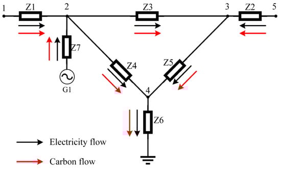
Figure 2.
Schematic diagram of the structure of carbon emission flows.
As shown in Figure 2, each generator set (e.g., wind farms or coal plants) and aggregated electricity demand area (typically representing industrial parks or urban districts) are modeled as nodes in the network. The transmission lines connecting these nodes constitute branches. Nodes 1 to 5 act as power load centers to consume electrical energy, while nodes 1 and 5 serve as connection points to the external microgrid. G1 is connected to node 2 in order to efficiently transmit the generated power to the rest of the system for regulating and controlling the distribution of power in the system. The ground (GND) represents the load balance and carbon emission balance of all power nodes in the system. As electrical energy is transmitted in the system, carbon flow is also transmitted along with electrical energy. Each branch consumes a certain amount of electrical energy when transmitting electrical energy due to the line resistance. Node carbon emission intensity and branch carbon emission intensity jointly construct the carbon emission flow analysis system of the power system to achieve full-chain tracking of the carbon footprint and energy–carbon collaborative optimization.
The CEF framework mandates that carbon responsibility allocation should originate from user-side analysis rather than conventional generator-centric approaches. By integrating topological power flow models with emission tracing algorithms, the CEF theory [] enables precise allocation of power generation-side carbon emission obligations to end-users, thereby establishing a causality chain from energy consumption to emission accountability.
2.2. Definitions Related to Carbon Flow Theory
2.2.1. Carbon Emission Flow Rate
The CEF rate represents the flow of CO2 through a node of the system per unit of time. Its unit is expressed as tCO2/h:
where represents flows of carbon emissions, and denotes time.
2.2.2. Branch Carbon Emission Intensity
The core mechanism of the carbon flow theory is rooted in the distributional characteristics of the active current in the power network. At the system operation level, a unit increment of electrical energy transmitted by any branch will lead to a corresponding increment of CO2 on the generation side. Branch carbon emission intensity (CEI) [], whose unit is tCO2/(KW·h), is calculated as follows:
where represents branch CEI of branch m, and denotes the active power of branch m.
2.2.3. Node Carbon Emission Intensity
Node CEI mainly describes the amount of CO2 generated on the power generation side due to node consumption per unit of electricity, which can be calculated as follows:
where represents all nodes connected to node j.
2.3. Carbon Emission Flow Calculation Method
According to the principle of proportional sharing [], in any outgoing node branch current, there exists a component of the inflow to that node branch current. The carbon flow rate of the outgoing branch active current shall be the sum of the carbon emission flows from all branches in the inflow node to branches flowing into that node. Taking node 2 in Figure 1 as an example, the node CEI of node 2 is calculated as follows []:
where indicates the active power of branch m at node 2; indicates the active power of node 2; represents branch carbon emission intensity of branch m at node 2; represents the CEF of the generator at node 2.
Under the theoretical framework of CEF, when the electric energy is transmitted along the network topology, the CEI of any power branch is directly determined by the CEI of its upstream head node.
According to the CEI of each generator at each node and the load capacity of each node of the system, the carbon emissions of each node can be solved.
where indicates the carbon emission of node i; represents the CEI of loading node i; is the load power of node i; represents the hours.
2.4. Dynamic Carbon Emission Calculation Model
In conventional carbon emission accounting methodologies, generator units are typically ascribed a constant emission coefficient that establishes a linear correlation between power generation and carbon emissions. This static quantification approach demonstrates diminishing accuracy over prolonged operational cycles due to its inability to precisely capture the inherent dynamic emission characteristics of thermal power generation systems under load-varying conditions. To address this limitation, an advanced piecewise–linear emission-intensity model is proposed, implementing load-dependent segmentation of the generator’s operational output. Through progressive refinement of load intervals under increasing generation capacity, the model exhibits stepwise attenuation characteristics in emission-intensity growth rates across operational regimes, as shown in Figure 3. Specifically, the nonlinear emission intensity curves are approximated by a multistage linearization method with interval division. As the generator approaches its rated power, the incremental marginal emission factor per unit of power output gradually decreases, thus improving the accuracy of the emission quantification under transient operating conditions. The carbon emissions are shaded in light green. The dynamic CEI is shown as a logarithmic function, which is the real curve to the approximate. Constant CEI is shown as the purple curve in the figure and does not change with increasing power. By constantly adjusting the number of intervals, the carbon emissions gradually approach the true curve.
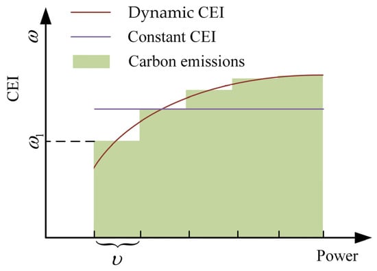
Figure 3.
Schematic of dynamic carbon emissions.
The specific calculation method of the dynamic carbon emission calculation model is as follows:
where indicates the total carbon emission of unit g at time t; represents the power output of unit g at time t; is the interval length; and represent the minimum and maximum output power interval length of unit q, respectively; indicates the lowest output power of the unit; represents the baseline value of CEI; represents the growth coefficient of carbon emission intensity, which gradually decreases with the gradual increase in carbon emission.
2.5. Multi-Phase Carbon Cost Calculation Model
The multi-phase carbon cost calculation mechanism is a segmented carbon accounting framework that leverages economic incentives to drive emission reductions. Its operational logic establishes multiple tiers based on user/enterprise carbon emission levels, with each tier assigned differential unit pricing coefficients. This structure exhibits a progressive pricing characteristic aligned with the principle that higher emission volumes correspond to elevated per-unit carbon costs. Its calculation model can be expressed as follows:
where indicates the total carbon emission cost of unit g at time t; represents the carbon emission cost coefficient; is the interval length; represents free carbon credits for generators, respectively; indicates the price increase in carbon cost between ranges, which is small.
3. Multi-Microgrid Optimal Scheduling
The MMG system composition contains () microgrid with autonomous regulation capabilities. The MMG modeling framework is shown in Figure 4. Each microgrid includes a diesel generator (DG), PV, WT, ESS, and electrical loads. Among the microgrid units, DG, PV, and WT act as active power generation units with the ability to directly inject electric power into the microgrid topology. ESS acts as a bi-directional energy buffer unit, which can either inject active power through the discharging mode or absorb excess power of the system through the charging mode. Its dynamic regulation characteristics effectively support the power balance and energy space–time transfer requirements of the microgrid. The system architecture is interconnected by power lines to form a cooperative operation network topology with N-1 redundancy characteristics, in which the MG realizes power interaction and voltage support through common connection points. The rest of the sections are summarized as follows: Section 3.1 presents the optimization objective function and constraints for the multi-microgrid model. Section 3.2 presents a MADRL-based approach to computational procedures.
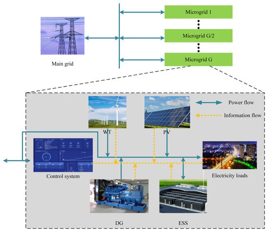
Figure 4.
The multi-microgrid modeling framework.
3.1. Optimal Scheduling Model
3.1.1. MMG Scheduling Objective Function
From a system operator’s perspective, the fundamental objective of online energy management resides in developing real-time adaptive control strategies to address the stochastic uncertainties arising from renewable generation intermittency and load–demand volatility. This operational paradigm necessitates tri-objective optimization through (1) carbon emission abatement via multi-energy complementarity coordination, (2) operational stability assurance through dynamic security-constrained optimal power flow, and (3) cost minimization via convex dispatch scheduling. Based on the consideration of the above factors, the following low-carbon economic optimization scheduling objectives are introduced:
where T denotes the number of timesteps; indicates the cost incurred in purchasing electricity from the main grid; stands for the cost incurred by the operation of the DG in the g-th microgrid; represents the cost of penalizing node voltage crossings. Discontinuities in function at certain points do not cause numerical problems in the subsequent algorithmic solution. denotes the power interaction between the main network and the MMG system; denotes the price of electricity at time t; indicates a timestep; and denote the fuel cost and operating cost of DG for the g-th microgrid system, respectively; denotes the working condition of DG; b, c, and d indicate the DG fuel cost factor; denotes the active power of the g-th DG at time t; indicates the cost of a change in the operating status of the g-th DG; denotes the voltage of the i-th node in the g-th microgrid at time t.
3.1.2. Constraints
The current dynamics across interconnected microgrids exhibit analogous mathematical formulations to those observed within individual microgrid subsystems. The power flow model framework primarily comprises four fundamental governing equations: branch voltage balance equations, active and reactive power balance equations at nodal injection points, and branch power transmission constraints.
where denotes the voltage magnitude at node i; indicates the resistance from node i to node j; stands for the reactance from node i to node j; represents the active power from node i to node j; denotes the reactive power from node i to node j; E represents the set of all the branches; N represents the set of all nodes; W represents all nodes connected to node i; denotes the magnitude of the current flowing from node i to node j.
In order to achieve power quality standards and ensure a reliable power supply, the nodal voltage should be kept within ±5% of the permissible range [,]. The upper and lower limits of nodal voltage are denoted as and , respectively, and the nodal voltage values are limited to the upper and lower limits:
For maintaining grid stability, generation-capable nodes must maintain operational boundaries within rigorously defined active–reactive power domains that satisfy both static and dynamic security constraints.
The PV active power range is defined as follows:
where denotes the active power injected into node i by the PV at time t, and indicates the maximum active power of the PV.
The WT active power range is defined as follows:
where denotes the active power injected into node i by the WT at time t, and indicates the maximum active power of the WT.
The ESS active power range is defined as follows:
where denotes the active power injected into node i by the ESS at time t, and indicates the maximum active power of the ESS.
The upper and lower bounds on the state of charge () of the ESS located at node i at time t are shown below:
where and indicate the maximum and minimum of the SOC separately.
The climbing restraints of the DG, i.e., the rate at which the DG increases or decreases the output power is subject to certain constraints, are determined as follows:
where indicates the maximum power of the g-th DG; denotes the active power produced by the g-th DG at node i at time t; and denote the rate of the climb for DG rising and descending, respectively; denotes the working condition of the g-th DG at time t, which is a binary variable (1: on; 0: off).
The relationship between the active power, reactive power, and capacity of the above equipment is shown below:
where indicates the maximum capacity of the device, and .
3.2. MADRL-Based Optimal Scheduling Approach
3.2.1. Markov Game Process
DRL is mathematically modeled through a Markov decision process, which contains three core elements: state, action, and reward. The learning mechanism is expressed as a continuous interaction process between the agent and the environment: at each discrete time step, the agent first perceives the current environment state and then chooses to perform an action based on the established policy. The action will trigger a change in the environment state through the state transfer function, and simultaneously, the environment will feed back a scalar reward as the behavioral evaluation. This ‘observation–decision–feedback’ loop mechanism enables the agent to gradually optimize its decision-making strategy through trial-and-error learning. For MMGs composed of multiple independent MGs (including G agents), it is necessary to construct a new scheduling framework based on stochastic game theory. Global optimization is achieved through strategic interaction among agents while taking into account both individual interests and system stability. This complex multi-objective coordination challenge can be rigorously formulated as a partially observable stochastic Markov game process [].
- Agent: Each microgrid comprises an agent;
- Environment: All the information on the microgrid;
- State: The state information required by each agent g at each time t is organized as follows:where indicate the information of the time series tariff in the past 24 h of the current time t; denote the total load information after summing the node loads for the past 24 h at the current time t; are the output timing data of the PV at node i; denote the output timing data of the WT at node i.
- Action: The agent action variables for the g-th microgrid are as follows:
- Reward: The optimization objective of the proposed control approach is to maximize the reward value. The reward for each agent is calculated as shown below:
- State transition function: The transfer function obtains the next state based on the currently acquired state , actions , and environment random variables .
3.2.2. Proposed Approach Based on MADRL
Traditional reinforcement learning methods (e.g., Q-learning []) exhibit computational inefficiency due to their dependence on an exhaustive Q-table traversal in discrete action spaces. To overcome this limitation, DRL employs neural networks to achieve continuous action space mapping. The twin-delayed deep deterministic policy gradient (TD3) algorithm implemented in this study extends the deep deterministic policy gradient (DDPG) framework, effectively mitigating the Q-value overestimation bias through its dual-network architecture with delayed updates []. Key algorithmic enhancements comprise three technical components: an alternating update protocol between independent critic networks, a delayed synchronization mechanism for target networks, and optimized policy update intervals. In the communication mechanism-enabled DRL called CommNet, each agent can only obtain its own state individually and then transmit it to the communication platform. Each agent can obtain the common average state (CAS) by accessing the propagated communication mechanism. The CAS is treated as the input to the subsequent layer, while the actions of each agent are generated by the final output layer []. The extended structure of CommNet is presented in Figure 5. Each row typically represents a different layer within the network. Each neuron in a layer is connected to every neuron in the subsequent layer, and the columns reflect these connections. These layers include input layers, hidden layers, and an output layer. The input layer receives the initial data (e.g., individual agent states). The hidden layers perform intermediate calculations and transformations, including the communication steps and , where agents share information. The output layer generates the final actions for each agent. The operations in the right-hand box of Figure 5 are performed based on Equation (34). Specifically, the operation is to add and and pass the result to the tanh activation function. is the result represented by the black line, which is processed by the linear transformation and the tanh activation function to be used for the next decision or strategy update. The blue line indicates the output of transmitted to the mean function. The red line indicates the output value after processing by the mean function.
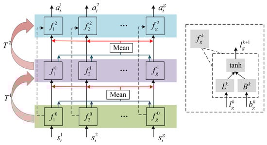
Figure 5.
The specific framework of CommNet.
The detailed calculations are shown below []:
where k represents the layers in the CommNet; is an activation function; represents the g-th agent for the k-th hidden layer vector; denotes the g-th agent for the k-th communication vector; is the g-th agent for the k + 1-th hidden layer vector; and indicate the coefficient matrices. Equation (34) can be further rewritten as follows:
where represents the coefficient matrices of k-th communication step.
3.2.3. Critic Network
The critic network of the CMMA-TD3 algorithm consists of two critic functions that compute the Q-value. Suppose is the result of the objective critic function. It is presented as follows:
where is the g-th agent value of the reward at moment t; denotes the discount factor; is the target critic function; is the all-agents state at time t + 1; represents the g-th agent action at time t + 1; denotes the g-th agent parameters of the target critic function.
The critic network loss function is denoted as follows:
where represents the mathematical expectation function.
The parameter gradients of the critic network are derived via gradient-based optimization techniques, mathematically formulated as follows:
where is the g-th agent decreasing gradient function of the critic network, and denotes the learning rate of the critic network.
3.2.4. Actor Network
The parametric formulation governing the policy function of the actor network can be mathematically represented as follows:
where denotes g-th agent parameters of the actor network.
The aforementioned mechanism consequently induces the mathematical derivation of the policy gradient for the actor network, formally expressed as follows:
where denotes the added noise in the target action function. This regularization mechanism mitigates premature convergence in the agent’s decision-making process by strategically injecting controlled Gaussian noise into both the policy parameterization and state-action value estimation, thereby circumventing suboptimal policy collapse through entropy-regularized optimization. represents the learning rate of the actor network.
The expression for the target actor function is shown below:
where denotes a noise in a normal distribution, represents variance, and is the value truncation position.
The temporal difference-driven optimization framework in actor–critic architectures operates through differentiable guidance from the critic network to the policy network. The significant divergence between the estimated state-action value and the target value function induces two critical failure modes: (1) policy gradient dispersion in the actor network due to high-variance advantage estimates and (2) value function approximation instability caused by non-stationary target distributions. To mitigate these coupled instabilities, delayed target network synchronization is implemented via the following:
where denotes the soft update factor, which can be constrained by to ensure stable temporal difference learning through quasi-static target propagation.
The specific computational flow of the proposed approach is illustrated in Figure 6.
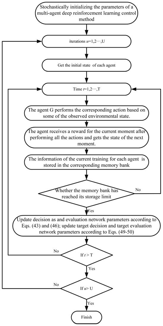
Figure 6.
The specific computational flow of the proposed approach.
4. Case Study
4.1. Dataset
In order to effectively verify the effectiveness of the proposed method, CMMA-TD3, we conducted training analysis in the MMG shown in Figure 7, which consists of three micromesh networks in total. The circuit parameters in the MMG system are shown in Table 1 []. The interconnected MGs contain three MGs, each of which contains ESS, WT, PV, and DG. Detailed calculation parameters of Section 3 in the MMG system are shown in Table 2 and Table 3 []. The parameter settings of the proposed scheme are shown in Table 4. In total, 200 days of training data and 30 days of test data were selected for the scheme proposed in this paper. The electricity load, WT, and PV-predicted power under typical scenarios are shown in Figure 8. MG1 serves as the primary load center with substantial renewable energy integration, characterized by elevated power consumption and a significant renewable energy generation capacity. MG2 exhibits reduced power consumption compared to MG1, coupled with a lower renewable energy generation capacity. MG3 demonstrates the highest renewable energy penetration among the three MGs while maintaining relatively modest electricity demand levels. The DG is the core device to ensure the power balance of the system, and its power output depends on the system’s demand. ESS, as a rechargeable and dischargeable device, mainly realizes the energy space–time transfer to improve the consumption of renewable energy.
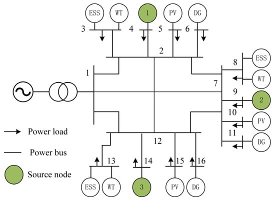
Figure 7.
Architecture of the MMG system.

Table 1.
The line parameters of the MMG system.
Table 2.
The parameters of the system.
Table 3.
The parameters of the MMG system.
Table 4.
Parameters of the proposed approach.
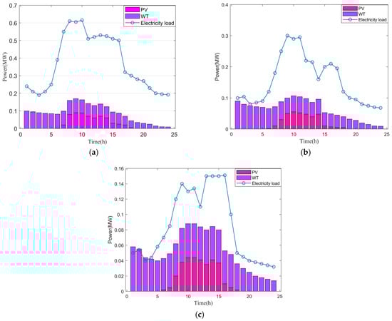
Figure 8.
Predicted power of the electricity load, PV, and WT of the MMG system. (a) Data of MG1; (b) data of MG2; (c) data of MG3.
4.2. Baselines
4.2.1. Benchmark Approaches
We evaluate the superiority of the presented methodology by employing multiple benchmarking methods for comparative analyses:
- (1)
- Particle swarm optimization algorithm (PSO) []: The particle constantly adjusts its speed and position according to its own historical optimal position and the global optimal position of the group, moves in the direction of the better solution, and finally, makes the group converge to the approximate optimal solution.
- (2)
- TD3: To enhance the performance and stability of DRL algorithms in continuous-action spaces, TD3 employs two critic networks to mitigate value-estimation bias and adopts a delayed-update strategy to stabilize the training process.
- (3)
- Multi-agent TD3 (MATD3) []: It is extended based on single-agent TD3. The core objective is to address the training instability problem in multi-agent body environments due to environmental non-stationarity and strategy coordination difficulties.
4.2.2. Performance in Training
As shown in Figure 9, this study compares the normalized cumulative reward values obtained during the training process of multiple reinforcement learning-based control methods. The convergence of the PSO training process is not demonstrated because the results of the PSO training process are quite different from the DRL-based method. It should be particularly noted that the agent does not have an a priori knowledge reserve during the early stage of decision-making, which forces the system to accumulate operational experience through the mechanism of action space exploration. With the advancement of training rounds, the agent gradually masters the energy management optimization strategy of the interconnected MMG system, which achieves the continuous gain of the reward function. It is worth noting that all the training curves show a monotonous upward trend until complete convergence, which indicates the termination of the training process.
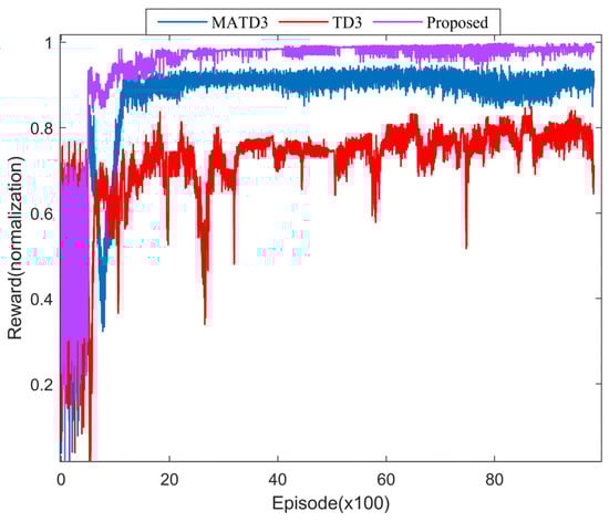
Figure 9.
The normalized cumulative reward of various methods.
During the training process, the TD3 algorithm exhibits the lowest benchmark value, and the results oscillate significantly. This demonstrates that when faced with the multi-dimensional co-optimization of MMG systems, its lack of a co-optimization mechanism results in an undesirable management strategy. MATD3 further improves the information interaction capability between MGs by introducing the multi-agent body framework, which leads to a more optimal scheduling strategy. The proposed approach further enhances the communication interaction between MGs by incorporating an information mechanism in the actor network to obtain the best performance.
4.2.3. Performance in Testing
Table 5 demonstrates the average cost and carbon emissions of the various methods over the 30 days of the test set. Compared with PSO, TD3, and MATD3, the operating cost of the proposed approach in the MMG system is reduced by 61.59%, 41.48%, and 24.08%, respectively, and the carbon emission of the proposed approach in the MMG system is reduced by 27.95%, 16.6%, and 7.72%, respectively. Due to the impossibility of PSO to accommodate all the constraints and the lack of synergy among MGs in the face of multi-objective optimization, its optimization effect shows the difficulty of traditional methods in obtaining excellent results in the face of complex power systems. TD3 further enhances the information interaction capability through the introduction of an agent, which is still insufficient to address the scheduling requirements of the MMG system. MATD3 further validates the necessity of multi-agents in MMG systems by introducing multi-agents. Compared to MATD3, the proposed approach demonstrates the optimal scheduling capability of MMG systems by enhancing the communication capability between agents.
Table 5.
The average cost and carbon emissions of various methods.
4.3. Performance on the Test Set over a Day
To further validate the effectiveness and generalization ability of the proposed approach, Figure 10 shows the scheduling strategy for a typical day. Figure 10a shows the real tariff for a typical day []. From Figure 8, it can be seen that MG1 has the lowest RES share and the lowest capability against voltage control. Therefore, the ESS1 exhibits a different scheduling strategy from the other two MGs, as shown in Figure 10b. MG1 exhibits characteristic voltage sag during the diurnal load ramping phase, necessitating its ESS to provide dynamic reactive power compensation. This countermeasure effectively mitigates voltage deviation propagation through controlled active power injection. In contrast, MG3′s configuration with a high renewable penetration ratio enables inherent voltage stabilization via RES inertia emulation. Such an operational paradigm permits ESS reallocation for energy arbitrage optimization, implementing time-of-use tariff-guided charging during off-peak periods and scheduled discharging at peak pricing intervals. The ESS2 is also able to profit by regulating the output under certain circumstances, but its behavior is more conservative compared to that of MG. As shown in Figure 10c, the SOC of the ESS3 at 18 h is smaller than that of the ESS2 at 24 h. Since the RES capacity of MG2 is smaller than that of MG3, the ESS needs more energy to stabilize the voltage in order to ensure the safety and stability of the MG2 system.
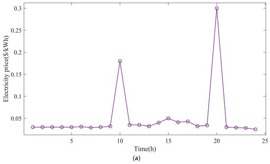
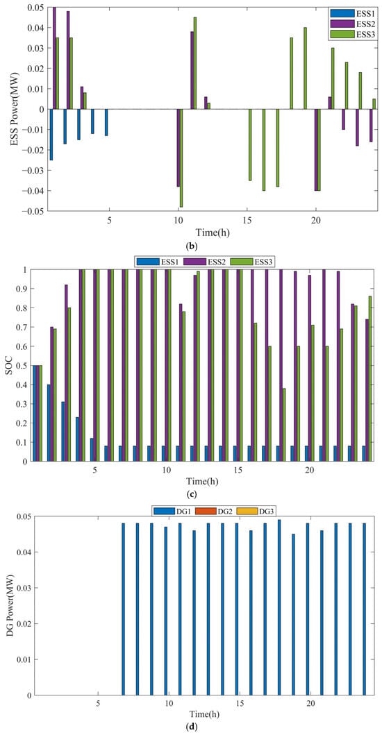
Figure 10.
Energy scheduling program for the proposed approach. (a) Electricity price; (b) power of ESSs in the MMG system; (c) energy of ESSs in the MMG system; (d) power of DGs in the MMG system.
The operation of DGs is shown in Figure 10d. The DG of MG1 hardly operates in the first six hours, and as the electricity load increases, the DG begins to operate nearly at full capacity. The first six hours almost maintain the stable operation of the MG1 system due to the small electrical load and energy replenishment from the ESS. As the load increases, it is difficult for MG1 to maintain the stability of the system, and DG is required to access the system to maintain the voltage. MG2 and MG3 do not require DG access as a way to reduce the operating cost after the strategy by scheduling optimization due to sufficient RES.
5. Conclusions
Aiming at the global low-carbon economy optimization problem of MMG systems, this research constructs a distributed coordination mechanism based on the CMMA-TD3 algorithm. Distinguishing from the traditional centralized scheduling’s reliance on global information sharing, this framework guides heterogeneous microgrid subjects to form a Pareto-optimal energy interaction pattern under the protection of data sovereignty by designing a marginal utility-driven incentive compatibility strategy. Specifically, the multi-energy co-optimization problem is modeled as a stochastic game process with incomplete information, in which each agent implements a distributed consensus protocol based on locally observed state-space mapping.
The analysis results in MMG show that (1) compared with the benchmark algorithms, PSO, TD3, and MATD3, the proposed method reduces the operation cost by 61.59%, 41.48%, and 24.08%, respectively, and reduces carbon emissions by 27.95%, 16.6%, and 7.72%, respectively. (2) Under the validation in the test set of 30 days, the proposed dispatch optimization method can develop optimal training results for the MMG system. (3) Under test set scenarios, the proposed method is more stable and achieves the best training results. The proposed scheduling optimization method is able to formulate the optimal control strategy for the MMG system. (4) The operation of the equipment within each microgrid further demonstrates that the optimization of the MMG internal coordination mechanism can effectively reduce the overall operation cost, which verifies the effectiveness of the proposed method.
Author Contributions
Data curation, M.Y.; Formal analysis, B.L. and M.Y.; Investigation, X.Y.; Methodology, B.L., M.Y., D.Z. and S.J.; Software, L.N. and B.L.; Supervision, S.J.; Visualization, D.Z. and X.Y.; Writing—original draft, L.N.; Writing—review and editing, L.N., D.Z. and S.J. All authors have read and agreed to the published version of the manuscript.
Funding
This research received no external funding.
Data Availability Statement
The data presented in this study are available on request from the corresponding author.
Conflicts of Interest
Lei Nie, Bo Long, and Meiying Yu were employed by the company State Grid Luzhou Power Supply Company. Dawei Zhang and Xiaolei Yang were employed by the State Grid Sichuan Electric Power Company. The remaining authors declare that the research was conducted in the absence of any commercial or financial relationships that could be construed as a potential conflict of interest.
References
- Zhao, P.F.; Hu, W.H.; Cao, D.; Huang, R.; Wu, X.W.; Huang, Q.; Chen, Z. Causal Mechanism-Enabled Zero-Label Learning for Power Generation Forecasting of Newly-Built PV Sites. IEEE Trans. Sustain. Energy 2025, 16, 392–406. [Google Scholar] [CrossRef]
- Yu, G.Z.; Zhang, Z.L.; Cui, G.A.; Dong, Q.; Wang, S.Y.; Li, X.C.; Shen, L.X.; Yan, H.Z. Low-carbon economic dispatching strategy based on feasible region of cooperative interaction between wind-storage system and carbon capture power plant. Renew. Energy 2024, 228, 120706. [Google Scholar] [CrossRef]
- Zhan, J.Y.; Wang, C.; Wang, H.H.; Zhang, F.; Li, Z.H. Pathways to achieve carbon emission peak and carbon neutrality by 2060: A case study in the Beijing-Tianjin-Hebei region, China. Renew. Sustain. Energy Rev. 2024, 189, 113955. [Google Scholar] [CrossRef]
- Cao, D.; Zhao, J.B.; Hu, W.H.; Huang, Q.; Chen, Z.; Blaabjerg, F. Data-driven multi-agent deep reinforcement learning for distribution system decentralized voltage control with high penetration of PVs. IEEE Trans. Smart Grid 2021, 12, 4137–4150. [Google Scholar] [CrossRef]
- Cao, D.; Hu, W.H.; Zhao, J.B.; Huang, Q.; Chen, Z.; Blaabjerg, F. A multi-agent deep reinforcement learning based voltage regulation using coordinated PV inverters. IEEE Trans. Power Syst. 2020, 35, 4120–4123. [Google Scholar] [CrossRef]
- IEA. Global Energy Review 2025 Dataset; IEA: Paris, France, 2025; Available online: https://www.iea.org/data-and-statistics/data-product/global-energy-review-2025-dataset (accessed on 25 March 2025).
- Zou, H.B.; Tao, J.; Elsayed, S.K.; Elattar, E.E.; Almalaq, A.; Mohamed, M.A. Stochastic multi-carrier energy management in the smart islands using reinforcement learning and un-scented transform. Int. J. Electr. Power Energy Syst. 2021, 130, 106988. [Google Scholar] [CrossRef]
- Dong, W.; Chen, C.F.; Fang, X.L.; Zhang, F.; Yang, Q. Enhanced integrated energy system planning through unified model coupling multiple energy and carbon emission flows. Energy 2024, 307, 132799. [Google Scholar] [CrossRef]
- Zhao, P.F.; Cao, D.; Hu, W.H.; Huang, Y.H.; Hao, M.; Haung, Q.; Chen, Z. Geometric Loss-Enabled Complex Neural Network for Multi-Energy Load Forecasting in Integrated Energy Systems. IEEE Trans. Power Syst. 2024, 39, 5659–5671. [Google Scholar] [CrossRef]
- Feng, Z.H.; Zhang, J.; Lu, J.; Zhang, Z.D.; Bai, W.W.; Ma, L.; Lu, H.N.; Lin, J. Low-Carbon Economic Dispatch Strategy for Integrated Energy Systems under Uncertainty Counting CCS-P2G and Concentrating Solar Power Stations. Energy Eng. 2025, 122, 1531–1560. [Google Scholar] [CrossRef]
- Wang, R.T.; Wen, X.Y.; Wang, X.Y.; Fu, Y.B.; Zhang, Y. Low carbon optimal operation of integrated energy system based on carbon capture technology, LCA carbon emissions and ladder-type carbon trading. Appl. Energy 2022, 311, 118664. [Google Scholar] [CrossRef]
- Gao, C.; Niu, K.; Chen, W.J.; Wang, C.W.; Chen, Y.B.; Qu, R. Novel Low-Carbon Optimal Operation Method for Flexible Distribution Network Based on Carbon Emission Flow. Energy Eng. 2025, 122, 785–803. [Google Scholar] [CrossRef]
- O’Shaughnessy, E.; Cruce, J.R.; Xu, K.F. Too much of a good thing? Global trends in the curtailment of solar PV. Sol. Energy 2020, 208, 1068–1077. [Google Scholar] [CrossRef] [PubMed]
- Yan, N.; Zhao, Z.J.; Li, X.J.; Yang, J.L. Multi-time scales low-carbon economic dispatch of integrated energy system considering hydrogen and electricity complementary energy storage. J. Energy Storage 2024, 104, 114514. [Google Scholar] [CrossRef]
- Hu, J.; Qin, K.; Ma, R.; Liu, W.X.; Zhang, J.Y.; Pang, L.M.; Zhang, J.W. A study on carbon emission flow tracking for new type power systems. Int. J. Electr. Power Energy Syst. 2025, 165, 110455. [Google Scholar] [CrossRef]
- Li, S.C.; Cao, D.; Hu, W.H.; Huang, Q.; Chen, Z.; Blaabjerg, F. Multi-energy management of interconnected multi-microgrid system using multi-agent deep reinforcement learning. J. Mod. Power Syst. Clean Energy 2023, 11, 1606–1617. [Google Scholar] [CrossRef]
- Yu, B.Y.; Fu, J.H.; Dai, Y. Multi-agent simulation of policies driving CCS technology in the cement industry. Energy Policy 2025, 199, 114527. [Google Scholar] [CrossRef]
- Zhao, B.; Wang, X.J.; Lin, D.; Calvin, M.M.; Morgan, J.C.; Qin, R.W.; Wang, C.S. Energy management of multiple microgrids based on a system of systems architecture. IEEE Trans. Power Syst. 2018, 33, 6410–6421. [Google Scholar] [CrossRef]
- Zhou, B.; Zou, J.T.; Chung, C.Y.; Wang, H.Z.; Liu, N.A.; Voropai, N.; Xu, D.S. Multi-microgrid energy management systems: Architecture, communication, and scheduling strategies. J. Mod. Power Syst. Clean Energy 2021, 9, 463–476. [Google Scholar] [CrossRef]
- Li, S.C.; Hu, W.H.; Cao, D.; Hu, J.X.; Chen, Z.; Blaabjerg, F. Coordinated operation of multiple microgrids with heat–electricity energy based on graph surrogate model-enabled robust multiagent deep reinforcement learning. IEEE Trans. Ind. Inform. 2025, 21, 248–257. [Google Scholar] [CrossRef]
- Wang, K.; Xue, Z.H.; Cao, D.; Liu, Y.; Fang, Y.P. Two-Stage Stochastic Resilience Optimization of Converter Stations Under Uncertain Mainshock-Aftershock Sequences. IEEE Trans. Power Syst. 2025, 1–13. [Google Scholar] [CrossRef]
- Zou, C.J.; Wang, K.; Xiahou, T.F.; Cao, D.; Liu, Y. Two-Stage Distributionally Robust Optimization for Infrastructure Resilience Enhancement: A Case Study of 220 kV Power Substations Under Earthquake Disasters. IEEE Trans. Reliab. 2024, 1–15. [Google Scholar] [CrossRef]
- Yi, Y.Q.; Xu, J.Z.; Zhang, W.M. A low-carbon driven price approach for energy transactions of multi-microgrids based on non-cooperative game model considering uncertainties. Sustain. Energy Grids Netw. 2024, 40, 101570. [Google Scholar] [CrossRef]
- Wang, Y.; Li, J.X.; Qu, D.Q.; Wang, X. Low-carbon economic operation strategy for a multi-microgrid system considering internal carbon pricing and emission monitoring. J. Process Control 2024, 143, 103313. [Google Scholar] [CrossRef]
- Cao, Z.H.; Li, Z.S.; Yang, C. Credible joint chance-constrained low-carbon energy Management for Multi-energy Microgrids. Appl. Energy 2025, 377, 124390. [Google Scholar] [CrossRef]
- Chen, H.P.; Yang, S.S.; Chen, J.D.; Wang, X.Y.; Li, Y.; Shui, S.Y.; Yu, H. Low-carbon environment-friendly economic optimal scheduling of multi-energy microgrid with integrated demand response considering waste heat utilization. J. Clean. Prod. 2024, 450, 141415. [Google Scholar] [CrossRef]
- Cao, D.; Zhao, J.B.; Hu, J.X.; Pei, Y.S.; Huang, Q.; Chen, Z.; Hu, W.H. Physics-informed graphical representation-enabled deep reinforcement learning for robust distribution system voltage control. IEEE Trans. Smart Grid 2024, 15, 233–246. [Google Scholar] [CrossRef]
- Cao, D.; Hu, W.H.; Zhao, J.B.; Zhang, G.Z.; Zhang, B.; Liu, Z.; Chen, Z.; Blaabjerg, F. Reinforcement Learning and Its Applications in Modern Power and Energy Systems: A Review. J. Mod. Power Syst. Clean Energy 2020, 8, 1029–1042. [Google Scholar] [CrossRef]
- Cao, D.; Hu, W.H.; Xu, X.; Wu, Q.W.; Huang, Q.; Chen, Z.; Blaabjerg, F. Deep reinforcement learning based approach for optimal power flow of distribution networks embedded with renewable energy and storage devices. J. Mod. Power Syst. Clean Energy 2021, 9, 1101–1110. [Google Scholar] [CrossRef]
- Li, S.C.; Hu, W.H.; Cao, D.; Hu, J.X.; Chen, Z.; Blaabjerg, F. A novel MADRL with spatial-temporal pattern capturing ability for robust decentralized control of multiple microgrids under anomalous measurements. IEEE Trans. Sustain. Energy 2024, 5, 1872–1884. [Google Scholar] [CrossRef]
- Ye, T.; Haung, Y.P.; Yang, W.J.; Cai, G.T.; Yang, Y.Y.; Pan, F. Safe multi-agent deep reinforcement learning for decentralized low-carbon operation in active distribution networks and multi-microgrids. Appl. Energy 2025, 387, 125609. [Google Scholar] [CrossRef]
- Xu, X.S.; Xu, K.; Zeng, Z.Y.; Tang, J.L.; He, Y.X.; Shi, G.Z.; Zhang, T. Collaborative optimization of multi-energy multi-microgrid system: A hierarchical trust-region multi-agent reinforcement learning approach. Appl. Energy 2024, 375, 123923. [Google Scholar] [CrossRef]
- Yang, T.; Xu, Z.M.; Ji, S.J.; Liu, G.L.; Li, X.H.; Kong, H.B. Cooperative optimal dispatch of multi-microgrids for low carbon economy based on personalized federated reinforcement learning. Appl. Energy 2025, 378, 124641. [Google Scholar] [CrossRef]
- Wang, C.; Wang, M.C.; Wang, A.Q.; Zhang, X.J.; Zhang, J.H.; Ma, H.; Yang, N.; Zhao, Z.L.; Lai, C.S.; Lai, L.L. Multiagent deep reinforcement learning-based cooperative optimal operation with strong scalability for residential microgrid clusters. Energy 2025, 314, 134165. [Google Scholar] [CrossRef]
- Yang, Y.; Takase, T. Spatial characteristics of carbon dioxide emission intensity of urban road traffic and driving factors: Road network and land use. Sustain. Cities Soc. 2024, 113, 105700. [Google Scholar] [CrossRef]
- Yang, X.H.; Li, L.X. A joint sharing-sharing platform for coordinating supply and demand resources at distributed level: Coupling electricity and carbon flows under bounded rationality. Appl. Energy 2025, 393, 126051. [Google Scholar] [CrossRef]
- Gao, X.; Zhang, J.H.; Chang, J.; Wang, S.Q.; Su, Z.A.; Mu, Z.Y. Employing battery energy storage systems for flexible ramping products in a fully renewable energy power grid: A market mechanism and strategy analysis through multi-Agent Markov games. Energy Rep. 2024, 12, 5066–5082. [Google Scholar] [CrossRef]
- Pang, X.F.; Fang, X.; Yu, P.; Zheng, Z.D.; Li, H.B. Optimal scheduling method for electric vehicle charging and discharging via Q-learning-based particle swarm optimization. Energy 2025, 316, 134611. [Google Scholar] [CrossRef]
- Wang, J.H.; Du, C.Q.; Yan, F.W.; Hua, M.; Gongye, X.Y.; Yuan, Q.; Xu, H.M.; Zhou, Q. Bayesian optimization for hyper-parameter tuning of an improved twin delayed deep deterministic policy gradients based energy management strategy for plug-in hybrid electric vehicles. Appl. Energy 2025, 381, 125171. [Google Scholar] [CrossRef]
- Zhang, Z.L.; Wan, Y.N.; Qin, J.H.; Fu, W.M.; Kang, Y. A deep RL-based algorithm for coordinated charging of electric vehicles. IEEE Trans. Intell. Transp. Syst. 2022, 23, 18774–18784. [Google Scholar] [CrossRef]
- Sukhbaatar, S.; Fergus, R. Learning multiagent communication with backpropagation. Neural Inf. Process. Syst. 2016, 29, 2244–2252. [Google Scholar]
- Du, W.Y.; Ma, J.; Yin, W.J. Orderly charging strategy of electric vehicle based on improved PSO algorithm. Energy 2023, 271, 127088. [Google Scholar] [CrossRef]
- Wang, X.; Zhou, J.S.; Qin, B.; Guo, L.Z. Coordinated control of wind turbine and hybrid energy storage system based on multi-agent deep reinforcement learning for wind power smoothing. J. Energy Storage 2023, 57, 106297. [Google Scholar] [CrossRef]
- PJM. Historical Hourly Electricity Price from PJM. May 2017. Available online: https://www.pjm.com/ (accessed on 15 March 2025).
Disclaimer/Publisher’s Note: The statements, opinions and data contained in all publications are solely those of the individual author(s) and contributor(s) and not of MDPI and/or the editor(s). MDPI and/or the editor(s) disclaim responsibility for any injury to people or property resulting from any ideas, methods, instructions or products referred to in the content. |
© 2025 by the authors. Licensee MDPI, Basel, Switzerland. This article is an open access article distributed under the terms and conditions of the Creative Commons Attribution (CC BY) license (https://creativecommons.org/licenses/by/4.0/).