AoI-Aware Resource Scheduling for Industrial IoT with Deep Reinforcement Learning

Abstract

Effective resource scheduling methods in certain scenarios of Industrial Internet of Things are pivotal. In time-sensitive scenarios, Age of Information is a critical indicator for measuring the freshness of data. This paper considers a densely deployed time-sensitive Industrial Internet of Things scenario. The industrial wireless device transmits data packets to the base station with limited channel resources under the constraints of Age of Information. It is assumed that each device has the capacity to store the packets it generates. The device will discard the data to alleviate the data queue backlog when the Age of Information of the data packet exceeds the threshold. We developed a new system utility equation to represent the scheduling problem and the problem is expressed as a trade-off between minimizing the average Age of Information and maximizing network throughput. Inspired by the success of reinforcement learning in decision-processing problems, we attempt to obtain an optimal scheduling strategy via deep reinforcement learning. In addition, a reward function is constructed to enable the agent to achieve improved convergence results. Compared with the baseline, our proposed algorithm can achieve better system utility and lower Age of Information violation rate.

1. Introduction

Timely data delivery services have garnered significant attention from the industry as an emerging field [1]. The demand for data freshness in IIoT has increased sharply with the rapid development of 5G communication technology. The performance of some IIoT services is determined by the freshness of data collected via equipment. Industrial devices continuously monitor the surrounding environment and transmit data updates to the controller via wireless networks such as temperature and humidity detection in warehouses and inspection of automated factory control [2]. These densely deployed services continue to generate a large amount of data and unreasonable scheduling in the case of limited channel resources may lead to device data backlog and affect quality of service. The significance of timely data updates is growing for the time-sensitive Industrial Internet of Things. Obsolete data can harm industrial applications, and outdated indicators may no longer meet current service requirements [3]. For instance, in an automated factory, wireless devices continuously monitor the environment and transmit data to the industrial control system. However, due to limited bandwidth, devices cannot transmit all the data in one time slot. As a result, the remaining data accumulate in a queue, causing a decrease in data freshness. The traditional delay indicator is insufficient in expressing the extent of data aging.

Age of Information is proposed as a novel metric for measuring data freshness. It is an end-to-end metric used to characterize latency in status update systems and applications [4]. Different from conventional metrics like latency or throughput, AoI is focused on information and considers both the effect of update delays and the rate of successful transmission [5]. AoI measures from a destination perspective the time that has elapsed between source generation and delivery of status updates. In [6], it is pointed out that the AoI of data decreases first and then increases with the acquisition frequency, while the delay keeps increasing. This suggests that reasonable resource scheduling is significantly important in keeping data fresh. In the Industrial Internet of Things, there are strict requirements for the freshness of sampled data. Optimizing the average AoI alone cannot completely prevent data from exceeding a predetermined AoI threshold [7]. Therefore, it is important to consider both average AoI and AoI violation rate optimization to ensure system stability. In addition, deep reinforcement learning is considered feasible for solving scheduling problems. DRL is a self-adaptive technique that can continuously improve its decision-making strategy in the process of continuous interaction with the environment, gradually approaching the optimal strategy [8]. The work in [9] identified the IIoT as one of the main application areas for DRL. DRL can automatically adjust policies based on changes in the environment, adapt to different system conditions and requirements and learn features and policies from original data without manual feature design. It has better ability when dealing with complex network resource scheduling problems and can handle unknown situations in resource scheduling. Performance can be enhanced by continuously learning and optimizing to adapt to changing network requirements and conditions. In this paper, we propose a DRL method to solve the intensive-deployment network optimization problem that combines network utility and minimization of average AoI and violation ratio. The DRL agent obtains the network status based on the number of devices and arrival rates. Then, at the given state, the agent is trained to find the optimal scheduling policy based on the environment reward.

The rest of this article is arranged as follows. Section 2 introduces the related research work. In Section 3, we introduce the system model of the IIoT scenario, the data queue model and the AoI queue model for each device. In Section 4, we describe the optimization objective and introduce the proposed deep reinforcement learning algorithm used for IIoT scenarios. The simulation results are presented in Section 5. Section 6 summarizes the research work and suggests the direction of future work.

2. Related Work

At present, there have been many studies on AoI. The study analyzed the average and peak AoI of multicast transmission in IoT systems [10]. The findings suggest that there exists an optimal deadline that minimizes the average AoI. The authors of [11] studied the optimal block length of a single server queue to minimize the AoI peak violation probability. It is important to note the significance of the AoI violation probability. In [12], the closure expression for peak AoI was derived in machine type communication device systems and set as the optimization target under state update rate and stability constraints. The study investigated the scenario where multiple IoT devices observe the same target together, using Age of Collection as a measure of data freshness, and analyzed the performance under three multi-access schemes [13]. A closed-form expression of average AoI based on two protocols in a collaborative IoT system was derived in [14]. The average transmission power of the sensor was minimized under the constraint of meeting the maximum average AoI for each sensor in [15]. A maximum generation time increment first scheduling strategy was proposed to reduce the total AoI of all sources in [16]. The study in [17] analyzed the scenario where a device is successfully updated and how this affects the AoI of other devices. The study aimed to minimize the average AoI of the system by reducing the AoI of other devices. A twin delayed deep deterministic policy gradient algorithm was proposed to minimize the average AoI of IoTDs in a UAV-assisted IoT network in [18]. The study in [19] proposed a nonlinear form of AoI penalty for multi-service systems that need to deploy different AoI functions and the results of the theoretical analysis are proved in wireless powered communication networks.

Lyapunov optimization and convex optimization techniques were commonly used to solve wireless resource scheduling. The author in [3] studied the scheduling problem in the Industrial Internet of Things network and used lyapunov and convex optimization techniques to achieve asymptotical closeness to optimal online decision making. The study in [20] considered data transmission and energy collection at different time granularity in Industrial Internet of Things networks. By using lyapunov optimization, the long-term stochastic optimization problem is transformed into a series of short-term deterministic optimization problems, and a low complexity rate control algorithm is developed to accelerate the convergence speed. A genetic algorithm was proposed to solve the decision-making process for flight path planning of UAVs in [21]. The author in [22] analyzed scheduling in a sleep–wake sensor network and proposed a max-weight-based scheduling policy to achieve the asymptotically optimal AoI lower limit while reducing energy consumption. As a promising method, deep reinforcement learning has been applied to network resource management many times. The DQN network has been widely used for resource allocation in wireless communication. In [23], DQNs were used for channel allocation in the D2D wireless network. However, only one state is mapped via DQN and the action space increases exponentially with the number of channels. The above algorithms cannot be applied to the resource-allocation problem in IIoT. DDPGs were used to solve the resource-allocation problem in scenarios of centralized wireless communication in [24]. However the DDPG is better suited for optimizing problems in continuous domains, such as power control. The work in [25] focused on mission-critical device-to-device communication in industrial wireless networks. The proposed approach utilized faith-based Bayesian reinforcement learning intelligence to establish a spectrum sharing alliance. The author in [26] studied link scheduling in wireless D2D communications. The integration neural network was proposed to learn mapping from geographic location information to optimal scheduling. The DDQN algorithm was employed in energy-limited IoT networks to obtain the optimal scheduling that balances the AoI and energy-consumption tradeoff in [27]. But it did not consider the system throughput, an important index to measure network service quality. Ref. [28] considered mobile edge computing system users to calculate offload and resource-allocation problems and used a DDPG deep reinforcement learning algorithm to optimize the energy consumption and offload tradeoffs in the system. A safe deep Q-network was used to dynamically select the unload strategy and the position perturbation strategy in [29]. The author in [30] studied the task offloading and resource-allocation problem in Maritime-IoT networks and proposed DDPG to optimize system-execution efficiency. In conclusion, reinforcement learning is suitable for solving industrial automation, resource scheduling and other related optimization problems.

Our paper studies the problem of wireless network resource scheduling in the Industrial Internet of Things. Due to the inevitable bandwidth limitation, the network cannot allow all devices to transmit the data stored in the buffer at the same time slot. Data transmission under poor channel state will cause a waste of resources and an unreasonable scheduling strategy will lead to a backlog of device data queue. Therefore, it is very important to select the appropriate scheduling strategy according to the data queue and channel state. We assume that all wireless devices share the spectrum in the way of TDMA. The AoI of the transmitted data must be kept within a certain threshold and our goal is to train a DRL agent to obtain the optimal scheduling policy to maximize the average system utility under different AoI constraints. The main contributions of this paper are as follows:

(1)

In order to improve the long-term average system utility with limited channel resources, we propose a new AoI and utility coordination method for IIoT by jointly considering data queue state, channel state and data freshness.

(2)

A DRL agent is trained to generate an optimal scheduling policy for IWD to transmit its data packets in each time slot. Based on the DDQN algorithm, we design an SDDQN algorithm which defines a more detailed reward function to make the agent converge faster.

(3)

We proposed a hybrid parameter update strategy base on a soft and hard copy to obtain a more stable convergence. We selected three evaluation indices, average system utility, average AoI and AoI violate ratio, to analyze the performance of our proposed algorithm. The simulation results suggest that our algorithm performs better under different AoI constraints.

3. System Model

Consider an IIoT communication system consisting of a set $\mathcal{N}=\{1,\dots ,N\}$ of industrial wireless devices and a base station as shown in Figure 1. Each IWD is equipped with an antenna for wireless communication and continuously detects physical process changes in the surrounding environment. The collected data are transmitted to the base station through the uplink. IWDs store the collected data in their own buffer pool in the format of data packets. The buffer maintains two queues: data queue and AoI queue, which store the generated data and the timestamp at the time of packet generation, respectively. Consider a time-slot-based TDMA system indexed by $t\in \{1,\dots ,T\}$ where the duration of each time slot is $\tau$. All IWDs share a set $\mathcal{K}=\{1,\dots ,K\}$ of orthogonal sub-channels with $\omega$ bandwidth per sub-channel [2]. Due to network resource limitations, we assume that $K<N$. The notations used in this article are summarized in Table 1.

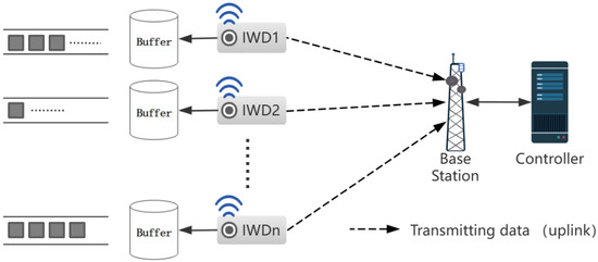
Figure 1. An Industrial Internet of Things network with N industrial wireless devices.

Table 1. List of Key Notations.

Notation	Definition
$n,k$	The IWD in set $\mathcal{N}$ and sub-channel in set $\mathcal{K}$
t	Time slot t and the length of a time slot
$\omega$	The bandwidth of sub-channel
$m_n\left(t\right)$	The channel allocation policy in time slot t
$P_0$	Transmit power of the device
$h_{n,k}\left(t\right)$	The channel gain of sub-channel k between IWDn and BS at time slot t
$SN{R}_{n,k}\left(t\right)$	The signal-to-noise ratio of device n in channel k at time slot t
$C_n\left(t\right)$	The transmission rate of device n at time slot t
$Q_n\left(t\right)$	Data queue backlog of device n at slot t
$D_n\left(t\right)$	Data dropped at device n at slot t
$a_n\left(t\right)$	The age of data collected at slot t by device n
$A_{max}$	The maximum value of AoI of device

At the beginning of each time slot, the central controller controls which IWD transmits the packets in the data queue. The scheduling strategy for time slot t is represented as $M\left(t\right)=\{m_1\left(t\right),m_2\left(t\right),\dots ,m_n\left(t\right)\},m_i\left(t\right)\in (0,1)$; $m_i\left(t\right)=1$ indicates that the IWDi is selected for transmitting the packets at t time slot; otherwise, $m_i\left(t\right)=0$. Accordingly, $m_i\left(t\right)$ satisfies:

$$\sum _{n=1}^N{m}_n\left(t\right)\le K,\forall n\in N$$

(1)

The uplink channels are presumed to be i.i.d which means the channel remains static in the single slot but changes in other time slots. We use $h_n\left(t\right)$ to denote the instantaneous channel gain between IWDn and BS in slot t. The controller accepts the pilot of the channel gain from each IWD at the beginning of the slot. The costs of signalling overhead are neglected. We assume the device is equipped with a reliable power capacity to transmit data packets. The transmission powers of device n are denoted by $P_0$. Hence, the $SNR$ of IWDn at slot t can be denoted by:

$$SN{R}_{n,k}\left(t\right)=\frac{P_0{h}_n^2\left(t\right)}{N_0\omega }$$

(2)

where $N_0$ and $\omega$, respectively, denote the power spectral density of the white Gaussian noise and the sub-channel bandwidth. Then, the transmission rate $C_n\left(t\right)$ can be represented as:

$$C_n\left(t\right)=\frac{\omega \tau }{L}{m}_n\left(t\right)lo{g}_2(1+\frac{P_0{h}_n^2\left(t\right)}{N_0\omega })n,k\in \mathcal{N},\mathcal{K}$$

(3)

where L is the length of packet in bits due to the packet characteristic in the industry [25].

At the beginning of time slot t, we use $a_n\left(t\right)$ to denote the data freshness of IWDn. $a_n\left(t\right)$ varies over slots and is modelled as i.i.d with a threshold $A_{max}$. The definition of AoI for IWDn is denoted by:

$$a_n\left(t\right)=t-max\left\{t_A^n\left(t\right)\right|t_D^n\left(i\right)\le t\}$$

(4)

where $t_A^n\left(t\right)$ and $t_D^n\left(i\right)$, respectively, denote the arrival and departure time of packets i of IWDn. Based on this, the evolution of AoI for IWD is denoted by:

$$a_n\left(t\right)=\left\{\begin{array}{cc}{a}_n(t-1)+1,\hfill & if{m}_n\left(t\right)=0\hfill \\ t-max\left\{t_A^n\left(t\right)\right|t_D^n\left(i\right)\le t\},\hfill & if{m}_n\left(t\right)=1\hfill \end{array}\right.$$

(5)

$A_{max}$ is indicated as the maximum age that the IIoT system can afford for the data packets. When $a_n\left(t\right)>A_{max}$, we reckon the data buffer backlog to be severe, that is no longer valuable and dropping the data that exceed the threshold to reduce the network load pressure. The AoI constraint is denoted by:

$$a_n\left(t\right)\le A_{max},\forall n\in \mathcal{N}$$

(6)

The generated data are stored in the data queue $Q_n\left(t\right)$ as packets following the first-come-first-serve (FCFS) policy. $g_n\left(t\right)$ denotes the packets that IWDn generated in time slot t, following the Poisson distribution process. We assumed that the packets generated at this time slot are not transmitted until the next time slot [3], so the dynamic evolution of the data queue is given by:

$$Q_n(t+1)=max\{Q_n\left(t\right)-C_n\left(t\right)-D_n\left(t\right),0\}+g_n\left(t\right)$$

(7)

where $D_n\left(t\right)$ denotes the packets needed to be dropped due to violation of the AoI threshold. The right side of the equation represents the data queue state after transmitting or dropping the data. Data transmitting will have higher priority than discarding data.

Due to the limited energy of devices, energy efficiency is also a metric that quantitatively evaluates the effectiveness of systems. In the industrial IoT system we considered, it is assumed that all devices use a constant transmit power. The EE of each device is denoted by [25]:

$$E_n\left(t\right)=\frac{C_n\left(t\right)}{P_0}$$

(8)

In order to obtain better system performance, throughput is not the only performance metric to consider; data freshness is also important in IIoT services. To tackle the data aging problem and improve the system service quality, we design the system utility in time slot t, denoted by:

$$U\left(t\right)=\sum _{n=1}^N{C}_n\left(t\right)-\alpha e^{\beta a\left(t\right)}-d_n\left(t\right)$$

(9)

where $\alpha ,\beta$ are constant parameters. The nonlinear form AoI penalty function is used to satisfy IIoT systems with different data sensitivity. For example, an exponential or logarithmic penalty function can be formed by adjusting $\alpha ,\beta$.

Consider the long-term average system performance; our purpose is finding a scheduling strategy to maximize the throughout and minimizing the AoI of data. Based on the above, the objective can be described as maximizing the system utility and formulated as:

$$\begin{array}{cc}\hfill P1:& max\sum _{t=1}^T\overline{U\left(t\right)}\hfill \\ \hfill & s.t.\left(1\right),\left(5\right),\left(6\right),\left(7\right)\hfill \end{array}$$

Obviously, P1 is a nonlinear programming problem which is complicated to solve using traditional optimization methods such as game-theoretic and heuristic methods. Recent research has shown that DRLs have great performance in long-term decision problems. We propose an SDDQN algorithm to search the optimal action selection strategy by an agent constantly interacting with its environment.

4. Proposed Deep Reinforcement Learning Algorithm

In this section, we will rephrase the problem as a Markov Decision Process (MDP) to make it easier to build DRL agents and then introduce our improved deep reinforcement learning algorithm for this model to generate an action policy to optimize the objectives.

4.1. MDP Formulation

The MDP can be denoted by $S,O,P,R$, where S denotes the set of environment states. O denotes the action set containing all actions during each time slot. P stands for state transition probability, which is the probability distribution of transitioning to the next state after taking action. R represents the reward that the agent will receive after taking an action in the current state.

Environment: The observation of environment mainly consists of three parts: data queue state vector $Q\left(t\right)$, age queue state vector $a\left(t\right)$ and channel gain vector $h\left(t\right)$. The variation in data queue and age queue follows the dynamic evolution which is determined by the previous action strategy. All of the above are passed to the agent to analyze and generate an action policy. The agent requested the observation and made a decision at each slot. Let $s\left(t\right)\in \mathcal{S}$ denote the state observed by the agent at slot t, represented as:

$$s\left(t\right)=({\left\{Q_n\left(t\right)\right\}}_{\forall n\in \mathcal{N}},{\left\{a_n\left(t\right)\right\}}_{\forall n\in \mathcal{N}},{\left\{h_n\left(t\right)\right\}}_{\forall n\in \mathcal{N}})$$

(10)

Actions: The agent generates a set of action vectors to control which devices to perform transmission at slot t. The vectors are represented by a set of discrete values with a range (0, 1). We use $o\left(t\right)$ to represent the action taken at slot t, denoted by:

$$o\left(t\right)=\left({\left\{m_n\left(t\right)\right\}}_{\forall n\in \mathcal{N}}\right)$$

(11)

Rewards: The reward function is a linear combination of the reward settlement from transitioning from the previous state s to the next state $s^{\prime }$. The reward components were data transmit incentive $R_t$, AoI penalty $R_a$, discard penalty $R_d$ and backlog penalty $R_b$.

Transmit bonus: The primary reward comes from the amount of packet transmitting in the time slot. In our study, we did not consider the effects of failed transmissions. We balanced the numerals of the transmit bonus to make the training converge better: $R_t=log(1+C\left(t\right))$. This reward item may decrease as the amount of data in queue is low, which indicates that the strategy executed by the agent is reasonable. Nevertheless, the agent may perceive this type of situation as bad due to the lower rewards. Therefore, we use a logarithmic function to reduce the precision loss caused by insufficient data.

AoI penalty: The AoI penalty was related to the freshness of data transmitted by IWDs. We set a non-linear penalty function to balance the weight of information freshness in making decisions: $R_a=\alpha e^{\beta \overline{a\left(t\right)}}$. The rate of penalty increase is controlled by the exponential function, where $\overline{a\left(t\right)}$ is the average AoI of transmitted packets. The exponential function was used to amplify the penalty of old data to meet some time-sensitive IIoT requirements.

Discard penalty: An agent may make several devices repeat data transmission in multiple consecutive time slots in order to obtain better rewards which results in a serious queue backlog on other devices. We set a discard penalty to assist the agent in learning to avoid intentionally discarding some devices with severe backlogs. The discard penalty was proportional to the amount of discarded data in the time slot: $R_d=D\left(t\right)$.

Backlog penalty: There is another situation that needs to be considered. When the current network channel status is relatively good and the data transmission situation is optimistic, there are fewer data in the queue of each device, which may result in less transmit reward. However, in the actual situation, this means that our strategy has achieved a good effect. To deal with this situation, the backlog penalty $R_b=\left({\sum }_{n=0}^N{Q}_n\left(t\right)\right|m_n\left(t\right)=0)$ represents the backlog of queues that are not transmitting in slot t. The $R_b$ was defined as a negative reward which it is hoped will become smaller in each slot.

In conclusion, the expression of the final reward function can be given as follows:

$$\begin{array}{cc}\hfill R\left(t\right)& =R_t-R_a-R_d-\lambda R_b\hfill \end{array}$$

(12)

The agent evaluates the performance of the policy via the long-term average cumulative reward $G\left(t\right)$, which is denoted by:

$$G\left(t\right)=\sum _{i=0}^{\infty }{\gamma }^{i}R(t+i)$$

(13)

where $\gamma$ is the discount factor.

4.2. Proposed SDDQN Algorithm

To address the problem of resource allocation in IIoT networks, we propose an algorithm based on SDDQN. The algorithm is implemented in the controller, which receives the observation state and makes scheduling decisions. We mainly improve two aspects: exploration strategy and parameter update policy. DQN performs well in solving low-dimensional discrete motion space problems, but overestimation may occur in training, resulting in sub-optimal solutions. We proposed a hybrid exploration strategy instead of epsilon-greedy exploration. $ϵ$-greedy exploration means that the agent has a probability of $ϵ$ to execute random action to explore the environment. The typical practice sets the hyperparameter $ϵ$ at the start of training and gradually reduces the value of $ϵ$ to a minimum value ${ϵ}_{min}$ with the increase of training times. In the hybrid exploration strategy, the target and eval neural network will replace epsilon greedy to output an action policy alternately when $ϵ$ is reduced to ${ϵ}_{min}$. The target and eval neural networks are used for action selection and action evaluation, respectively. DQN deals with high dimension state spaces by introducing neural networks but produces overestimation of the action-value function. By decomposing the max operation into action selection and action evaluation, the overestimation problem can be effectively reduced. The eval network, with parameter $\theta$, generates the action, while the target network, with parameter ${\theta }^{-}$, evaluates the action.

$$o^{max}\left(s_{t+1}\right)=\underset{o}{argmax}Q(s_{t+1},o_t;\theta )$$

(14)

$$Q_{target}=R_t+\gamma Q(s_{t+1},\underset{o}{argmax}{Q}_{eval}(s_{t+1},o_t;\theta );{\theta }^{-})$$

(15)

$$Q_{eval}=Q(s_t,o_t;\theta )$$

(16)

The first term on the right-hand side in (14) represents the reward for taking an action $o_t$ in state $s_t$. The agent enters the next state $s_{t+1}$ into Eval Q to obtain different Q values, and then selects the action $o_{t+1}$ corresponding to the largest Q value. Later, the agent inputs $s_{t+1}$ into Target Q to find the value corresponding to action a as the actual network value and the predicted value is expressed as $Q_{eval}$. A loss function is defined to measure the difference between predicted and actual value. It is denoted as follows.

$$L\left(\theta \right)=E\left[{(Q_{target}-Q_{eval})}^2\right]$$

(17)

To prevent instability caused by updating predicted and target values simultaneously in the loss function, the target network update policy will not update with eval network. The DQN usually uses asynchronous Hard updating. After N-step training, the target network updates parameters from the Eval network. In our proposed hybrid update policy, we extend the N-step size of hard updating and the soft updating is added during the N-step. This lagging update method ensures the speed and stability of training convergence. The parameter update method is shown in (17):

$${\theta }_{target}=\left\{\begin{array}{c}{\theta }_{eval}ifepoc{h}_{n}mod{N}_{step}=0\hfill \\ \varphi {\theta }_{eval}+(1-\varphi ){\theta }_{target}else\hfill \end{array}\right.$$

(18)

where $\tau$ is the proportional constant. The SDDQN reinforcement learning algorithm details are summarized in Algorithm 1.

Algorithm 1 SDDQN for resource scheduling in Industrial Internet of Things

Input: $P_0$, $N_0$, $\omega$, L, $\tau$, $\alpha ,\beta ,\lambda ,\varphi$

1: Initializing eval network parameters $\theta$ and target network parameter ${\theta }^{-}$ 2: Initializing learning rate, discount factor, batch size 3: for epoch = 1,2,3,… do 4:    Get initial state $s\left(t\right)$ from environment 5:    for t = 1,2,3,… do 6:      if $ϵ>{ϵ}_{min}$ then 7:         select a random action $o\left(t\right)$ with probability $ϵ$ 8:         otherwise $o\left(t\right)=\underset{o}{argmax}Q(s\left(t\right),o;{\theta }^{-})$ 9:      else 10:         Eval network and Target network output $o\left(t\right)$ alternately 11:      end if 12:      Execute action $o\left(t\right)$,get reward $r\left(t\right)$ and next state $s_{t+1}$ 13:      Store transition($s\left(t\right),o\left(t\right),r\left(t\right),s(t+1)$) in experience pool, if the pool is full, discarding the earliest samples 14:      Sample random batch of transition from experience pool 15:      Computer $Q_{target}$ by (14) 16:      Use MSE loss function and Adam optimization algorithm to update the eval network parameter $\theta$ 17:      ${\theta }^{-}\leftarrow \varphi \theta +(1-\varphi ){\theta }^{-}$ 18:      update the ${\theta }^{-}$ to be the same as $\theta$ after N steps 19:    end for 20: end for

5. Evaluation and Simulation Results

5.1. Simulation Setup

In this section, the simulation results are provided to evaluate the performance of the proposed algorithm, where the relevant parameter is based on the settings in [3,19,25,27]. The experiment parameters are shown in Table 2.

Table 2. The simulated parameters.

Parameter	Value
Packet size L	256 Byte
Slot duration $\tau$	2 ms
Bandwidth W	0.2 MHz
Transmission power $P_0$	2 W
White Gaussian noise $N_0$	30 dBm
Learning rate	5 × ${10}^{-5}$
Batch Size	128
Hybrid update step $N_{step}$	200

The BS is in the center of the industrial scenario and twenty industrial wireless devices are randomly distributed around the BS with a range of [100, 200] m. The wireless channels are affected by the Rayleigh fading model which is set as $h_n\left(t\right)={10}^{-3}{d}^{-\psi }{h}^{-}\left(t\right)$, where $\psi$ is the path-loss exponent and $h^{-}\left(t\right)$ is an exponentially distributed random variable which denotes the short-term fading [3]. For each device, we have $\psi =2$ and $N_0={10}^{-9}$ W. The size of the packets is 1024 bits and the transmit power is set as $P_0=2$ W.

The neural network of SDDQN consists of three fully connected layers with 1024 units each and ReLU was used as an activation function between two layers. The network parameters update via the Adam optimizer and the learning rate is set to 5 × ${10}^{-5}$. The mixing updating parameter $\varphi$ was set to 0.005, $\gamma$ = 0.99, and the backlog penalty $\lambda$ was set to 0.1. The experience replay pool capacity was set to 1000 and a dependence experiment consists of 50 time slots.

In actual deployment, the observed environmental state data are preprocessed to adapt to the input requirements of the proposed algorithm. Then, the data from each time slot are stored in the experience replay buffer for subsequent model training. The training dataset is generated by sampling batch from the replay buffer. The trained models are deployed into the IIoT environment and optimized in real time to adapt to the changing environment. The performances of the model are monitored in the real environment and the performance of the model is evaluated to make adjustments and optimizations periodically. There may be the following problems in the actual implementation process: 1. Poor data quality affects the ability of data training and generalization. 2. The decision process belongs to the black box model, which may cause trust and interpretation problems in the industrial IoT.

5.2. Simulation Results

We consider three baselines to compare with our proposed algorithm, namely round robin, greedy and DQN, and primarily validate the performance of our proposed algorithm through three aspects: system utility, average AoI and AoI violation ratio.

(1)

Round Robin (RR): All sub-channels are assigned to each device in turn.

(2)

Greedy: All sub-channels are allocated based on the current backlog status of the device’s data queue.

(3)

Deep Q-Network (DQN): The sub-channel allocation strategy is generated by the RL agent with the relevant network parameters of the agent being the same as SDDQN.

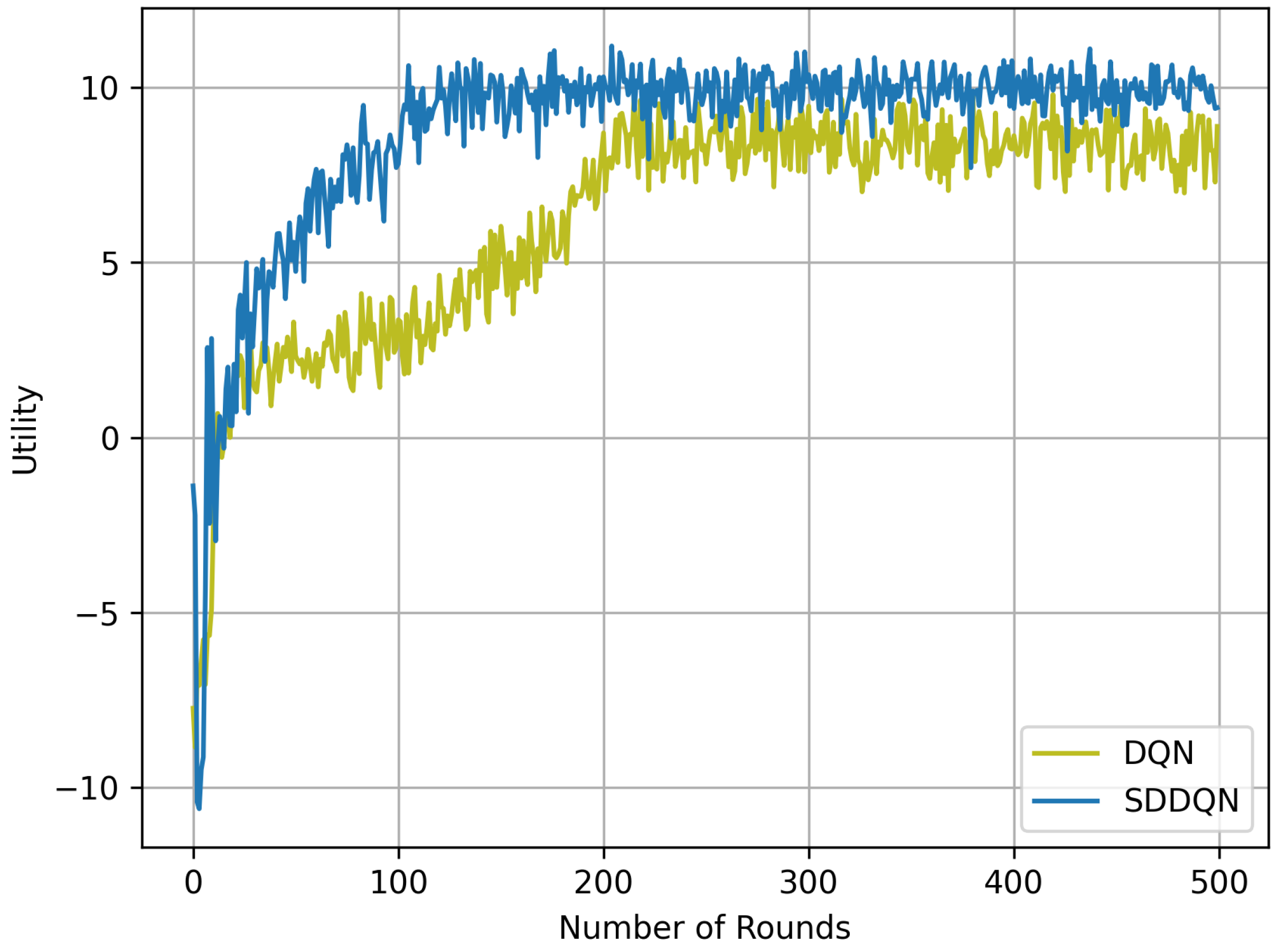
Figure 2 illustrates the performance curve of our proposed algorithm compared to the DQN algorithm where the channel number is 10 and $A_{max}=5$. It can be seen in the figure that the performance of the two DRL algorithms gradually become stable after a period of learning. Because of the hybrid exploration strategy and parameter updating, the SDDQN algorithm can achieve a faster convergence speed than DQN, which converges to the optimal value in 150 independent experiments. Although the SDDQN curve exhibited several poor performances after convergence, our proposed algorithm outperforms the DQN strategy in long-term system average utility. In addition, our proposed algorithm has a smaller and more stable range of fluctuations than DQN.

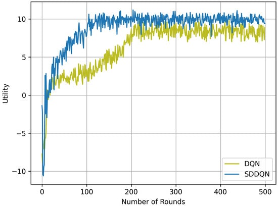
Figure 2. Utility and convergence rate comparison between SDDQN and DQN.

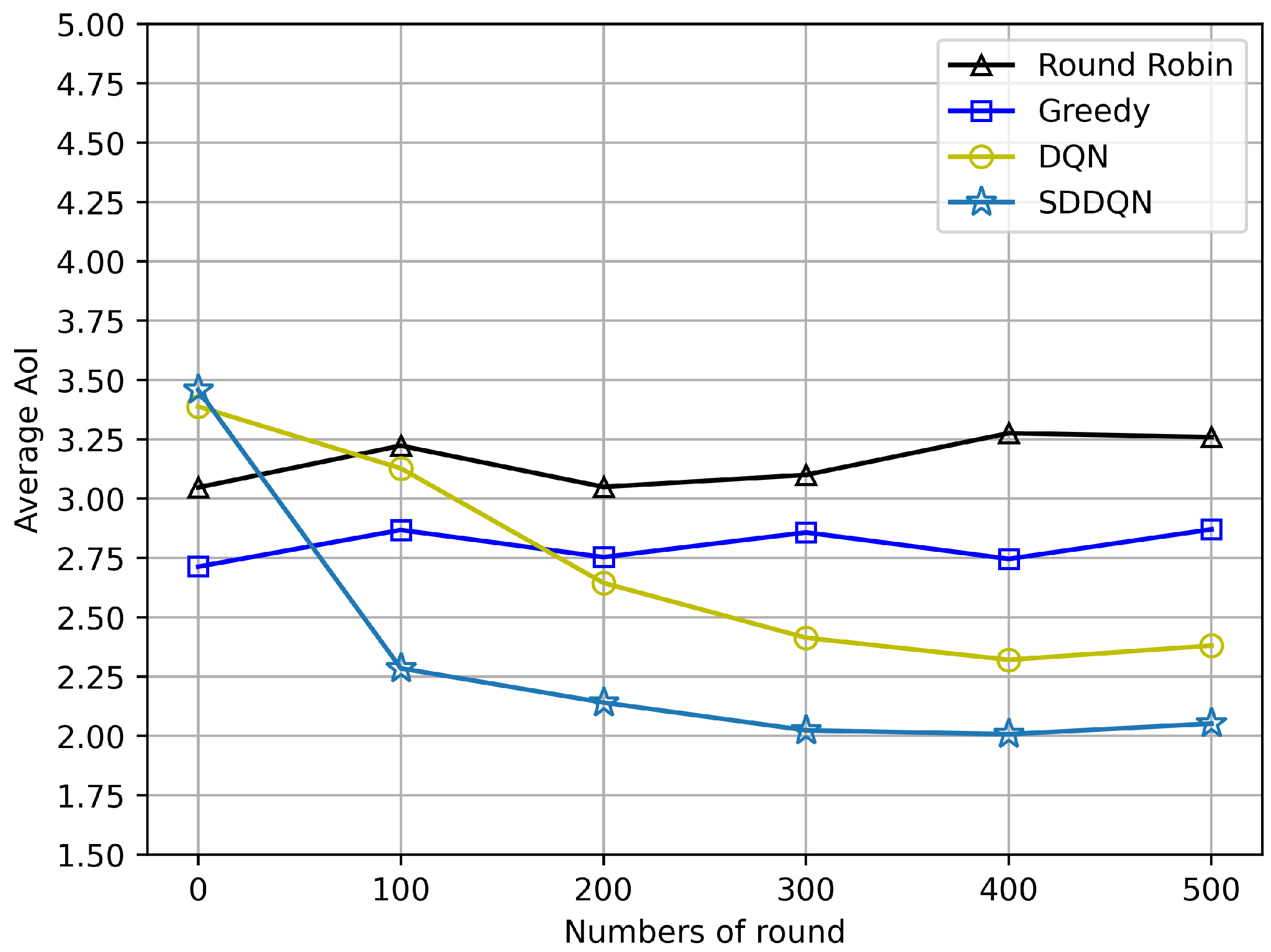
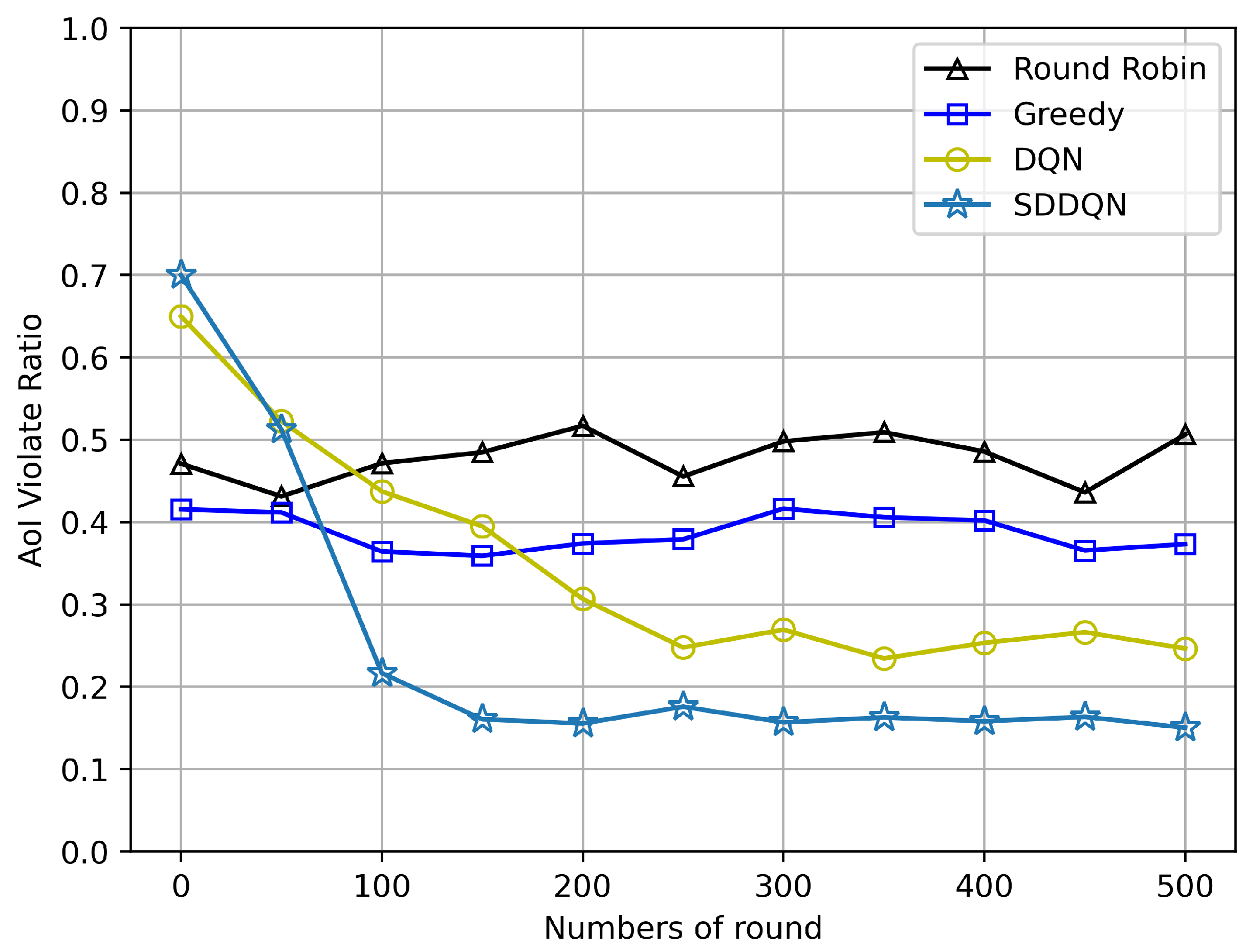
Figure 3 and Figure 4 depict comparisons of the average AoI and the AoI violation ratio for four algorithms, respectively. The average AoI of each algorithm is lower than the AoI threshold due to the consideration of timeout discarding. With the gradual convergence of the agent, the average AoI of the SDDQN and DQN algorithm gradually decreases and tends to be stable. It can be concluded from both figures that SDDQN outperforms other algorithms due to the hybrid exploration and update strategy. Even though the average AoI performance is not significantly improved, our proposed algorithm can enhance the device’s AoI violation rate performance when the system channel resources are limited and data freshness is required.

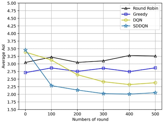
Figure 3. Average AoI comparison (N = 20, K = 10, $A_{max}$ = 5).

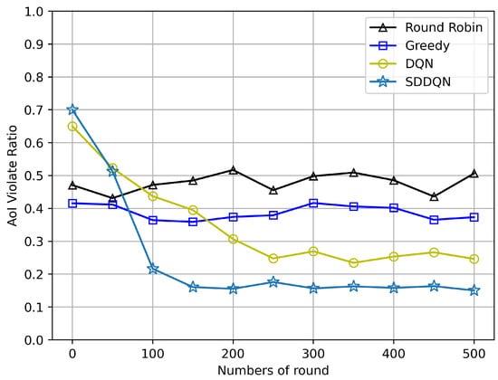
Figure 4. AoI violation ratio comparison (N = 20, K = 10, $A_{max}$ = 5).

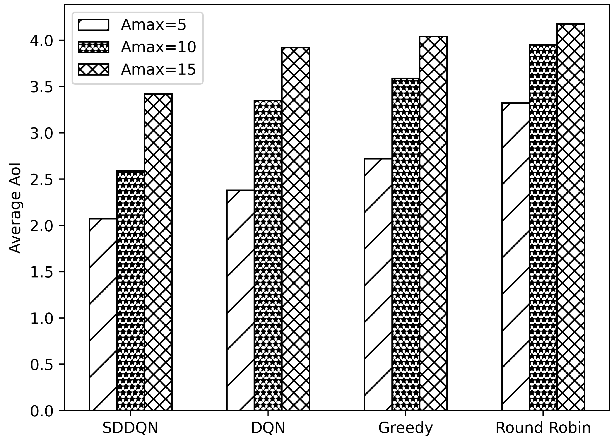
Figure 5 and Figure 6, respectively, illustrate comparisons of the average system utility and average AoI for the four algorithms under varying data freshness requirements. In Figure 5, the system utility of all algorithms increases as the threshold of AoI rises. The reason for this is that when the system’s data age requirements are lowered, the data backlog caused by insufficient channel resources is resolved in the following few slots. This reduces the number of times that the device drops data and improves the overall system utility. Additionally, with increases in the AoI threshold, the average AoI also increases. Combining Figure 5 and Figure 6, when the AoI threshold rises to 15, there are very few timeout data in the queue of the device. The growth of data AoI affects the overall utility of the system.

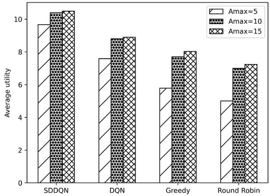
Figure 5. Average utility comparison under varying thresholds of AoI.

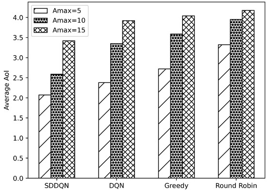
Figure 6. Average AoI comparison under varying thresholds of AoI.

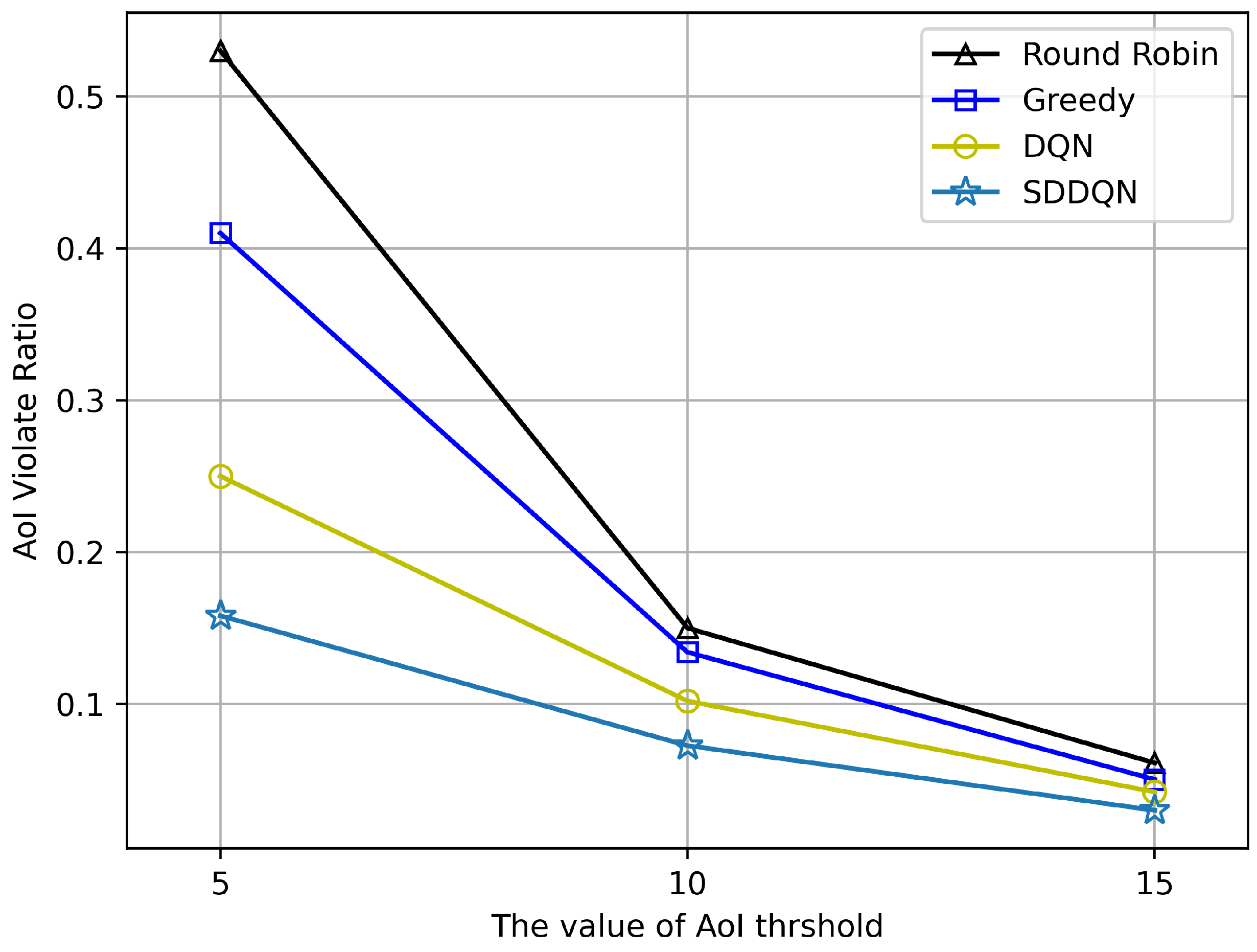
Figure 7 shows the performance of AoI violation rate under different values of $A_{max}$. With increases in the value of the threshold, the violation rate of AoI decreases gradually. When $A_{max}=15$, all algorithms can achieve a lower violation performance. It also can be observed in Figure 7 that our proposed algorithm can make more better scheduling decisions when the system requires high data freshness.

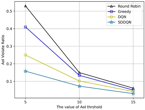
Figure 7. AoI violation ratio at different threshold (N = 20, K = 10).

6. Conclusions

In this paper, we studied the resource allocation for wireless devices in the Industrial Internet of Things. Under the constraint of AoI, we propose an SDDQN algorithm to train agents to generate action policies. We aimed to maximize the average system utility and translate the problem into a Markov decision process. The major limitation of the present study is the existing sample bias. DRL is a self-learning technique that generates datasets by sampling small batches from the experience replay buffer. This can lead to poor generalization of DRL models after training. The proposed method has certain reference value in densely deployed IIoT networks that are sensitive to data freshness. The scalability of the proposed algorithm in large-scale industrial IoT is mainly affected by the number of devices and network resources. The input scale of the proposed algorithm increases by $3n$, where n represents the number of system devices. In addition, as the system scale increases, the number of network neurons should also increase to achieve better performance and generalization ability. In simulation experiments, it is generally necessary to gradually increase the number of neurons and observe the system performance to find the appropriate network scale.

In future work, we will further consider the energy consumption of devices with limited energy. Current applications of reinforcement learning have better results for specific scenarios. The convergence speed and portability of the algorithm are the next improvement directions.

References

- Chen, C.; Lyu, L.; Zhu, S.; Guan, X. On-Demand Transmission for Edge-Assisted Remote Control in Industrial Network Systems. IEEE Trans. Ind. Inf. 2020, 16, 4842–4854. [Google Scholar] [CrossRef]
- Wu, C.-C.; Popovski, P.; Tan, Z.-H.; Stefanovic, C. Design of AoI-Aware 5G Uplink Scheduler Using Reinforcement Learning. In Proceedings of the 2021 IEEE 4th 5G World Forum (5GWF), Virtual, 13–15 October 2021; pp. 176–181. [Google Scholar]
- Wu, H.; Tian, H.; Fan, S.; Ren, J. Data Age Aware Scheduling for Wireless Powered Mobile-Edge Computing in Industrial Internet of Things. IEEE Trans. Ind. Inf. 2021, 17, 398–408. [Google Scholar] [CrossRef]
- Yates, R.D.; Sun, Y.; Brown, D.R.; Kaul, S.K.; Modiano, E.; Ulukus, S. Age of Information: An Introduction and Survey. IEEE J. Sel. Areas Commun. 2021, 39, 1183–1210. [Google Scholar] [CrossRef]
- Grybosi, J.F.; Rebelatto, J.L.; Moritz, G.L.; Li, Y. Age-Energy Tradeoff of Truncated ARQ Retransmission with Receiver Diversity. IEEE Wirel. Commun. Lett. 2020, 9, 1961–1964. [Google Scholar] [CrossRef]
- Sun, Y.; Uysal-Biyikoglu, E.; Yates, R.D.; Koksal, C.E.; Shroff, N.B. Update or Wait: How to Keep Your Data Fresh. IEEE Trans. Inf. Theory 2017, 63, 7492–7508. [Google Scholar] [CrossRef]
- Pu, C.; Yang, H.; Wang, P.; Dong, C. AoI-Bounded Scheduling for Industrial Wireless Sensor Networks. Electronics 2023, 12, 1499. [Google Scholar] [CrossRef]
- Giannopoulos, A.; Spantideas, S.; Capsalis, N.; Gkonis, P.; Karkazis, P.; Sarakis, L.; Trakadas, P.; Capsalis, C. WIP: Demand-Driven Power Allocation in Wireless Networks with Deep Q-Learning. In Proceedings of the 2021 IEEE 22nd International Symposium on a World of Wireless, Mobile and Multimedia Networks (WoWMoM), Pisa, Italy, 7–11 June 2021. [Google Scholar]
- Chen, Y.; Liu, Z.; Zhang, Y.; Wu, Y.; Chen, X.; Zhao, L. Deep Reinforcement Learning-Based Dynamic Resource Management for Mobile Edge Computing in Industrial Internet of Things. IEEE Trans. Ind. Inform. 2021, 17, 4925–4934. [Google Scholar] [CrossRef]
- Li, J.; Zhou, Y.; Chen, H. Age of Information for Multicast Transmission With Fixed and Random Deadlines in IoT Systems. IEEE Internet Things J. 2020, 7, 8178–8191. [Google Scholar] [CrossRef]
- Devassy, R.; Durisi, G.; Ferrante, G.; Simeone, O.; Uysal-Biyikoglu, E. Delay and Peak-Age Violation Probability in Short-Packet Transmissions. In Proceedings of the 2018 IEEE International Symposium on Information Theory (ISIT), Vail, CO, USA, 17–22 June 2018; pp. 2471–2475. [Google Scholar]
- Fang, Z.; Wang, J.; Ren, Y.; Han, Z.; Poor, H.; Hanzo, L. Age of Information in Energy Harvesting Aided Massive Multiple Access Networks. IEEE J. Sel. Areas Commun. 2021, 5, 1441–1456. [Google Scholar] [CrossRef]
- Liang, J.; Chan, T.-T.; Pan, H. Minimizing Age of Collection for Multiple Access in Wireless Industrial Internet of Things. IEEE Internet Things J. 2024, 11, 2753–2766. [Google Scholar] [CrossRef]
- Li, B.; Wang, Q.; Chen, H.; Zhou, Y.; Li, Y. Optimizing Information Freshness for Cooperative IoT Systems with Stochastic Arrivals. IEEE Internet Things J. 2021, 8, 14485–14500. [Google Scholar] [CrossRef]
- Moltafet, M.; Leinonen, M.; Codreanu, M.; Pappas, N. Power minimization for Age of Information constrained dynamic control in wireless sensor networks. IEEE Trans. Commun. 2022, 1, 419–432. [Google Scholar] [CrossRef]
- Hoang, L.; Doncel, J.; Assaad, M. Age-oriented scheduling of correlated sources in multi-server system. In Proceedings of the 2021 17th International Symposium on Wireless Communication System (ISWCS), Berlin, Germany, 6–9 September 2021. [Google Scholar]
- Tong, J.; Fu, L.; Han, Z. Age-of-information oriented scheduling for multichannel IoT systems with correlated sources. IEEE Trans. Wirel. Commun. 2022, 11, 9775–9790. [Google Scholar] [CrossRef]
- Zhang, J.; Kang, K.; Yang, M.; Zhu, H.; Qian, H. AoI-minimization in UAV-assisted IoT Network with Massive Devices. In Proceedings of the 2022 IEEE Wireless Communications and Networking Conference (WCNC), Austin, TX, USA, 10–13 May 2022. [Google Scholar]
- Hu, H.; Xiong, K.; Lu, Y.; Gao, B.; Fan, P.; Letaief, K.B. α–β AoI Penalty in Wireless-Powered Status Update Networks. IEEE Internet Things J. 2022, 9, 474–484. [Google Scholar] [CrossRef]
- He, Y.; Ren, Y.; Zhou, Z.; Mumtaz, S.; Al-Rubaye, S.; Tsourdos, A.; Dobre, O.A. Two-Timescale Resource Allocation for Automated Networks in IIoT. IEEE Trans. Wirel. Commun. 2022, 21, 7881–7896. [Google Scholar] [CrossRef]
- Xiong, J.; Li, Z.; Li, H.; Tang, L.; Zhong, S. Energy-Constrained UAV Data Acquisition in Wireless Sensor Networks with the Age of Information. Electronics 2023, 12, 1739. [Google Scholar] [CrossRef]
- Wang, J.; Cao, X.; Yin, B.; Cheng, Y. Sleep–Wake Sensor Scheduling for Minimizing AoI-Penalty in Industrial Internet of Things. IEEE Internet Things J. 2022, 9, 6404–6417. [Google Scholar] [CrossRef]
- Junjie, T.; YingChang, L.; Lin, Z.; Gang, F. Deep Reinforcement Learning for Joint Channel Selection and Power Control in D2D Networks. IEEE Trans. Wirel. Commun. 2021, 20, 1363–1378. [Google Scholar] [CrossRef]
- Xu, Y.-H.; Yang, C.-C.; Hua, M.; Zhou, W. Deep deterministic policy gradient (DDPG)-based resource allocation scheme for NOMA vehicular communications. IEEE Access 2020, 8, 18797–18807. [Google Scholar] [CrossRef]
- Li, M.; Chen, C.; Hua, C.; Guan, X. Learning-Based Autonomous Scheduling for AoI-Aware Industrial Wireless Networks. IEEE Internet Things J. 2020, 7, 9175–9188. [Google Scholar] [CrossRef]
- Luo, L.; Liu, Z.; Chen, Z.; Hua, M.; Li, W.; Xia, B. Age of Information-Based Scheduling for Wireless D2D Systems with a Deep Learning Approach. IEEE Trans. Green Commun. Netw. 2022, 3, 1875–1888. [Google Scholar] [CrossRef]
- Li, M.; Wang, Y.; Zhang, Q. Deep Reinforcement Learning for Age and Energy Trade off in Internet of Things Networks. In Proceedings of the 2022 IEEE/CIC International Conference on Communications in China (ICCC), Foshan, China, 11–13 August 2022; pp. 1020–1025. [Google Scholar]
- Nath, S.; Wu, J. Deep reinforcement learning for dynamic computation offloading and resource allocation in cache-assisted mobile edge computing systems. Intell. Converg. Netw. 2020, 1, 181–198. [Google Scholar] [CrossRef]
- Min, M.; Liu, Z.; Duan, J.; Zhang, P.; Li, S. Safe-Learning-Based Location-Privacy-Preserved Task Offloading in Mobile Edge Computing. Electronics 2023, 13, 89. [Google Scholar] [CrossRef]
- Wei, Z.; He, R.; Li, Y.; Song, C. DRL-Based Computation Offloading and Resource Allocation in Green MEC-Enabled Maritime-IoT Networks. Electronics 2023, 12, 4967. [Google Scholar] [CrossRef]
Disclaimer/Publisher’s Note: The statements, opinions and data contained in all publications are solely those of the individual author(s) and contributor(s) and not of MDPI and/or the editor(s). MDPI and/or the editor(s) disclaim responsibility for any injury to people or property resulting from any ideas, methods, instructions or products referred to in the content. |
© 2024 by the authors. Licensee MDPI, Basel, Switzerland. This article is an open access article distributed under the terms and conditions of the Creative Commons Attribution (CC BY) license (https://creativecommons.org/licenses/by/4.0/).