Transformer Core Fault Diagnosis via Current Signal Analysis with Pearson Correlation Feature Selection

Abstract

The role of transformers in power distribution is crucial, as their reliable operation is essential for maintaining the electrical grid’s stability. Single-phase transformers are highly versatile, making them suitable for various applications requiring precise voltage control and isolation. In this study, we investigated the fault diagnosis of a 1 kVA single-phase transformer core subjected to induced faults. Our diagnostic approach involved using a combination of advanced signal processing techniques, such as the fast Fourier transform (FFT) and Hilbert transform (HT), to analyze the current signals. Our analysis aimed to differentiate and characterize the unique signatures associated with each fault type, utilizing statistical feature selection based on the Pearson correlation and a machine learning classifier. Our results showed significant improvements in all metrics for the classifier models, particularly the k-nearest neighbor (KNN) algorithm, with 83.89% accuracy and a computational cost of 0.2963 s. For future studies, our focus will be on using deep learning models to improve the effectiveness of the proposed method.

1. Introduction

Predictive maintenance (PM) is a cutting-edge approach that leverages data-driven methodologies to anticipate potential equipment or machinery failures. This proactive technique enables timely maintenance measures by gathering data from strategically placed sensors or analyzing current and voltage levels, minimizing any unforeseen downtime. PM has become an essential tool for efficient and cost-effective operations because it can predict and prevent potential equipment breakdowns [1,2]. The prevalence of data-driven strategies compared to model-based methodologies is often credited to the difficulties of creating and maintaining precise physics-of-failure models. The importance of a data-driven approach when training artificial intelligence (AI) models must be considered in PM. This approach plays a crucial role in unlocking the complete potential of AI-based models, guaranteeing their effectiveness in anticipating and averting equipment malfunctions [3,4].

Condition-based maintenance (CBM) has emerged as a pivotal strategy in ensuring transformers’ reliability and optimal performance in modern power systems. Transformers are critical in power distribution, stepping up or down voltage levels for efficient energy transfer. As transformers are subjected to various operational stresses, the early detection of potential faults or deterioration is paramount to prevent catastrophic failures and minimize downtime [5]. CBM leverages advanced monitoring and diagnostic techniques, such as real-time data acquisition, signal analysis, and predictive modeling, to assess the health status of transformers. This proactive approach enables timely intervention, reducing maintenance costs, enhancing operational efficiency, and extending the lifespan of transformers. In complex power distribution systems, transformers play a pivotal role in ensuring the efficient transmission of electrical energy. However, these critical components are susceptible to faults compromising reliability and performance. One of the most crucial fault types is related to the transformer core, which forms the heart of its operation. Core faults encompass issues such as insulation degradation, winding deformations, and, most notably, the presence of cracks [6].

During the initial stages of a core fault, the transformer may not be affected significantly. However, the damage can become more severe over time if left unchecked. It is essential to conduct preventive evaluations for possible failures, especially core faults, to ensure a reliable energy supply. This can effectively minimize the risk of further damage to the transformer, resulting in shorter outages and reduced repair costs [7,8]. Furthermore, given the high cost of transformers and the challenges associated with their maintenance, early fault detection is of paramount importance to facilitate timely repairs, ultimately reducing the risk of significant breakdowns [9,10,11].

This study investigated a 1 kVA transformer in both healthy and faulty states, utilizing electric current data. Distinct current behavior in these states is a crucial indicator of fault patterns, especially in advanced stages. Detecting faults in raw data can be challenging, particularly during early fault development. To address this, signal processing becomes pivotal for implementing condition monitoring, offering data compression, noise reduction, and pattern recognition. A filter-based statistical feature selection approach, including Pearson correlation, is applied for efficient feature selection in time-domain analysis. This enhances precision and allows a more comprehensive observation of faults through various analyses, such as time-domain, frequency-domain, time–frequency, and Pearson-correlation-based statistical feature selection, contributing to proactive maintenance and improved reliability in power electronics systems [12,13,14,15,16].

This study introduces a novel model for identifying core faults in transformers by leveraging electric current data to assess the health of the transformer core. These contributions collectively advance the comprehension of transformer health assessment, laying the foundation for more effective fault detection methodologies in power systems. The study offers the following significant contributions:

• We have designed an experimental setup with the aim of collecting current signals, which should serve as a baseline for other researchers in analyzing transformer core fault analysis.
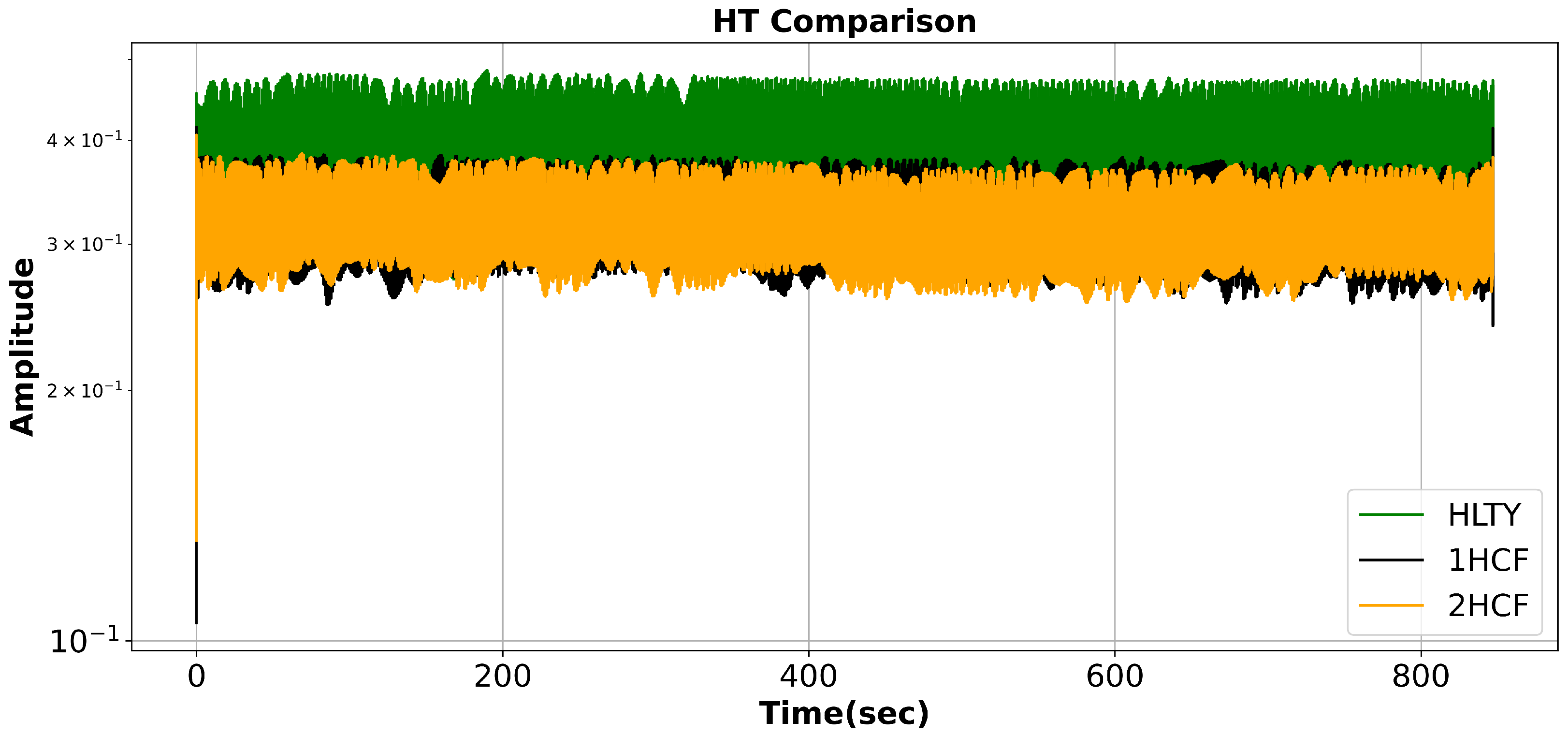
• We applied the Hilbert transform, a time-domain signal processing technique, to extract the magnitude envelope. This step is critical in improving the interpretation of signal analysis.
• We have established a comprehensive framework for robust feature engineering, focusing on extracting time-domain statistical features and filter-based Pearson correlation feature selection.
• We have conducted a comparative analysis in terms of performance evaluation to validate the efficiency of the proposed framework.

The subsequent sections of the paper are organized as follows: Section 2 delves into a review of related works and provides insight into the motivation behind the study, while Section 3 explores the theoretical background of the research. Section 4 presents the system model of the proposed fault diagnosis framework. Section 5 provides details on the testbed setup and collection of data. The detailed experimental results of the study are discussed in Section 6, and the paper concludes in Section 7, where the findings are summarized and future works are discussed.

2. Motivation and Review of the Related Literature

The basic working principle of a transformer lies in the usage of alternating current. When an alternating current flows to a winding, it generates a magnetic field in the core, thus inducing voltage in the secondary side. This is possible through the concept of electromagnetic induction. The core provides a path for the magnetic flux generated by the primary winding. It is commonly made of laminated thin sheets of electrical steel so that the layers are insulated from each other, which reduces eddy current losses, improving the transformer’s efficiency. When a magnetic field changes within a conductor, circulating currents called eddy currents are induced within the core. These currents circulate in closed loops and result in the generation of heat due to the electrical resistance of the material [17,18]. As stated in [11], the core fault is one of the common failures in transformers, which is the main motivation of this study. Table 1 summarizes various core faults, including brief descriptions, causes, and effects studied in [19,20], namely, saturation and lamination faults, respectively. In this study, we focus on mechanical damage to the transformer core.

Table 1. Different types of transformer core fault.

Type	Description	Cause	Effect
Saturation	Occurs when the magnetic flux reaches its limit	Overloading, sudden changes in load, or system faults	Overheating, and distorted output waveform
Lamination fault	Deterioration of insulation between laminations	Aging, excessive moisture, or manufacturing defects	Potential short circuit and reduced insulation resistance
Mechanical damage	Physical damage to the core, such as bending or cracking	Mechanical stress, operational stress, or overloading	Altered magnetic properties, increased core losses

Research on data-driven fault detection of transformers’ health created a new perspective for researchers as a new approach. However, only a few focused on using machine learning (ML) algorithms to develop predictive models. In [21], the authors presented a method for analyzing core looseness faults by acquiring vibration signals and used different time–frequency analysis methods to compare which method worked well. However, based on the mode of the dataset collected (vibration signal) and the study’s goal, the wavelet and empirical mode decomposition performed better than the other techniques under study. Another development in transformer fault analysis is the usage of the feature extraction method on vibration signals based on variational mode decomposition, and Hilbert transform (HT) is applied to obtain the Hilbert spectrum of the signal [22]. Interestingly, in [20], detection and classification of lamination faults, namely, edge burr and lamination faults, were analyzed. They extracted average, fundamental, total harmonic distortion (THD), and standard deviation (STD) features from the collected current signal and fed them to SVM, KNN, and decision tree (DT) algorithms.

The authors in [23] addressed the issue of acquiring precise data on vibrations and acoustics by developing a simulation technique for transformer core fault detection based on multi-field coupling. They validated their simulation results through physical experiments. However, no noise reduction technique was implemented in the data collection process, which may lead to the inclusion of unwanted signals. Advanced techniques in machine learning and signal processing have revolutionized the way we approach fault detection and prognosis modeling. The paper [24] presents a remarkable case in which these techniques were applied to develop a prognosis model for a transformer based on vibration signals. In addition, the paper [25] offers an online method that utilizes vibration measurements to distinguish the condition of the transformer core. Notably, the researchers in [12,26] also demonstrated the effectiveness of an electric current and Pearson correlation filter-based statistical feature selection approach in analyzing faults in moving machines such as motors. These findings highlight the potential of advanced signal processing and machine learning techniques to revolutionize the field of fault detection and prognosis modeling.

The current signal is a crucial diagnostic tool in power electronics, especially when identifying faults in components like transformers. By carefully analyzing variations in the current signal, experts can gain valuable insights into potential issues, enabling them to diagnose faults quickly and accurately. This is essential for maintaining the reliability and longevity of power electronic systems. In [27], they presented different machine-learning-based methods for diagnosing faults in electric motors. The first method used short-time Fourier transform (STFT) analysis on stator phase current signals for demagnetization fault diagnosis in permanent magnet synchronous motor (PMSM) drive systems, with high accuracy results obtained using k-nearest neighbors (KNNs) and multilayer perceptron (MLP) models. Similarly, in [28], they explored fault diagnosis in wind turbines (WTs) using electrical signals from the generator of a 20-year-old operating WT. For this, signal analysis techniques such as fast Fourier transform (FFT) and periodogram were employed to compare the effectiveness of spectral analysis methods, demonstrating the feasibility of using current signals for fault detection. Interestingly, in [29], the focus shifted to induction motor (IM) fault diagnosis through the stator current and delved into advanced signal processing tools. It showed the efficacy of spectrogram, scalogram, and Hilbert–Huang transforms in detecting rotor failures under various conditions, offering insights into fault diagnosis during transient operations. Also, in [30], they proposed a novel approach for rotor speed estimation in squirrel cage induction motors. This method employed signal processing techniques on airgap signals measured by a Hall effect sensor and compared the fast Fourier transform and Hilbert transform to traditional stator current methods. The results revealed superior accuracy in estimating rotational speed, especially in scenarios involving broken rotor bars—Hall effect sensors. After comparing FFT and HT with traditional stator current methods, the research indicated superior accuracy in estimating rotational speed, particularly in scenarios involving broken rotor bars.

We have integrated signal processing with intelligent algorithms, employing FFT and Hilbert transform. While deep learning methods like class-aware adversarial multiwavelet convolutional neural networks [31] yield accurate results, signal processing adds value by extracting meaningful features from raw data [32,33]. This combination enhances the model’s interpretability and performance, bridging the gap between complex signals and effective machine learning outcomes. The goal is to understand the impact of varied preprocessing strategies on model outcomes.

2.1. Analysis Concerning Time Domain and Frequency Domain

Analyzing signals is of paramount importance in various scientific and engineering applications, and understanding the time and frequency domains is fundamental to this analysis. In the time domain (TD), examining signals provides insights into their temporal behavior, allowing researchers and engineers to understand how the signal varies with respect to time. This is crucial for assessing the transient response of systems, studying the duration and shape of pulses, and investigating dynamic behaviors such as switching events. TD analysis is essential for evaluating the stability, response time, and overall performance of circuits and systems [34]. In the frequency domain (FD), analysis reveals the frequency components present in the signal. This is particularly valuable for characterizing harmonic content, identifying resonances, and assessing the spectral distribution of the current. FD analysis is indispensable in the design and optimization of power distribution systems, as well as in identifying and mitigating issues related to electromagnetic interference and power quality [35].

2.2. Overview of Selected Machine Learning Algorithms

This comprehensive overview illuminates the diverse capabilities of these machine learning models in solving real-world problems. The AdaBoost classifier (ABC) is a versatile algorithm for categorization, assembling numerous simple decision-makers to form a robust classifier focusing on correcting past mistakes to mitigate overfitting [36]. The k-nearest neighbors (KNNs) algorithm classifies new data points by assessing the labels of their ‘k’ closest neighbors, excelling in both classification and regression tasks [37,38,39]. Logistic regression (LR) is a straightforward method for binary choice scenarios, particularly effective when the relationship between features and target group is uncomplicated [40]. The multilayer perceptron (MLP) adapts during learning tasks by adjusting its layers to enhance predictive capabilities, managing non-convex loss functions and local minima fluctuations [41]. Stochastic gradient descent (SGD) efficiently trains learning models, rapidly improving accuracy after each example, balancing speed and precision [42]. Support vector machines (SVMs) excel in intricate grouping and prediction scenarios, particularly identifying optimal group separation [43].

3. Theoretical Background

3.1. Fast Fourier Transform

The fast Fourier transform (FFT) is a signal processing technique designed for computing the discrete Fourier transform (DFT). To comprehend the intricacies of DFT, it is essential to first delve into the concept of Fourier transform (FT). FT analyzes a signal in the time domain, breaking it down into a representation that exposes its frequency components. It explains the extent to which each frequency contributes to the original signal. Furthermore, FT within a discrete time domain is referred to as DFT, and FFT is recognized as an algorithm specifically tailored for the rapid computation of a large number of DFTs. The FT of a function, denoted as f(t), is shown below [44,45]:

$$\mathcal{F}\left\{f\left(t\right)\right\}=F\left(\omega \right)={\int }_{-\infty }^{\infty }f\left(t\right)e^{-j\omega t}dt$$

(1)

The FFT employs complex exponentials or sinusoids of varying frequencies as its basis functions, effecting a transformation into a distinct set of basis functions. Originally devised as an enhancement to the conventional DFT, the FFT significantly diminishes computational complexity from $\left(N^2\right)$ to $(NlogN)$, rendering it especially beneficial for efficiently processing extensive datasets and real-time applications. Mathematically, the FFT can be succinctly expressed as [46]

$$X\left(k\right)=\sum _{n=0}^{N-1}x\left(n\right)·e^{-\frac{2\pi i}{N}kn},k=0,1,2,\dots ,N-1$$

(2)

3.2. Hilbert Transform

The derivation of an analytic signal from a real-valued signal entails the utilization of the Hilbert transform (HT). The resultant analytic signal finds widespread application in signal processing and communication systems, serving diverse purposes such as analyzing frequency content, extracting envelope information, and facilitating phase-sensitive operations [47,48]. The HT of a real-valued signal $f\left(t\right)$ is given by

$$H\left[f\left(t\right)\right]\left(t\right)=\frac{1}{\pi }{\int }_{-\infty }^{\infty }\frac{f\left(\tau \right)}{t-\tau }d\tau$$

(3)

or in terms of the Cauchy principal value:

$$H\left[f\left(t\right)\right]\left(t\right)=\frac{1}{\pi }\underset{ϵ\to 0^{+}}{lim}\left[{\int }_{-\infty }^{t-ϵ}\frac{f\left(\tau \right)}{t-\tau }d\tau +{\int }_{t+ϵ}^{\infty }\frac{f\left(\tau \right)}{t-\tau }d\tau \right]$$

(4)

The analytic signal $F_H\left(t\right)$, combining the original signal $f\left(t\right)$ and its HT, is given by

$$F_H\left(t\right)=f\left(t\right)+j·H\left[f\left(t\right)\right]\left(t\right)$$

(5)

The properties of analytical signal include:

• Complex representation: The analytic signal is complex, with both real and imaginary components. The actual component signifies the original signal, while the imaginary component represents the Hilbert transform of the signal.
• A 90-degree phase shift: The positive frequency shifts to a negative 90-degree angle, and the negative frequency shifts to a positive 90-degree angle in the context of HT. This introduces a phase shift of 90 degrees between the original signal and its HT, which is crucial in applications such as demodulation and phase-sensitive analysis. Additionally, the analytic signal, derived through the HT, provides a representation of the original signal that separates positive and negative frequency components. This property is valuable for analyzing the frequency content of a signal.
• Enveloping: The envelope of the original signal can be extracted from the magnitude of the analytic signal. The envelope represents the slowly varying magnitude of the signal and is useful in applications such as amplitude modulation.

4. Proposed Diagnostic Framework

This section presents the process for detecting faults in transformers, as illustrated in Figure 1. The following stages are involved: gathering current dataset from both the healthy and faulty states of the transformer; applying signal processing methods, in particular, Hilbert transform; performing statistical feature extraction in the time domain to extract relevant features; using a Pearson correlation filter-based approach to identify highly correlated features; using the selected features for model training and testing; and lastly, carrying out performance evaluation to confirm the model’s effectiveness.

Figure 1. Proposed fault diagnosis framework.

It is imperative to represent data in a simplified manner, emphasizing only essential features before inputting them into the model to enhance the speed and accuracy of an ML model. Time-domain statistical features are extracted to capture the relevant aspects of the data. The primary objective of this process is dimensionality reduction while retaining crucial properties or features. Moreover, transforming the raw data into a more concise representation yields several advantages, including improved overall model performance by reducing complexity, decreasing computational time, and mitigating the risk of overfitting. In this study, we employ feature engineering through statistical feature extraction, and the 14 extracted features in the time domain and 13 in the frequency domain are illustrated in Table 2 and Table 3.

The linear relationship between two variables can be statistically measured on a scale ranging from −1 to 1. If the value is close to 1, they are highly correlated, and the sign indicates a positive or negative correlation. Negative values indicate a negative correlation, signifying that as one variable increases, the other decreases. Conversely, positive values suggest a positive correlation, meaning that both variables increase or decrease simultaneously. A value of 0 denotes no correlation between the variables. This approach is widely employed in data analysis, statistics, and ML for feature selection and comprehending the relationships between variables [49,50]. The formula is presented below:

$$r=\frac{\mathrm{cov}(X,Y)}{{\sigma }_X·{\sigma }_Y}$$

(6)

Table 2. Time-domain statistical features and formulas [51].

Domain	Features	Formulas
Time-based	Crest Factor	$\frac{\mathrm{Peak} \mathrm{Value}}{\mathrm{RMS} \mathrm{Value}}$
	Form Factor	$\frac{\mathrm{RMS} \mathrm{Value}}{\mathrm{Mean} \mathrm{Value}}$
	Interquartile Range	$Q_3-Q_1$
	Margin	$\frac{\mathrm{Peak} \mathrm{Value}}{\mathrm{Mean} \mathrm{Value}}$
	Max	$\frac{\mathrm{Peak} \mathrm{Value}}{\mathrm{Mean} \mathrm{Value}}$
	Mean	$\frac{{\sum }_{i=1}^N{x}_i}{N}$
	Median Absolute Deviation	$median\left(\right|x_i-median\left(x\right)\left|\right)$
	nth Percentile (5, 25, 75)	100$\frac{\mathrm{x}-0.5}{\mathrm{n}}$
	Peak-to-peak	$x_{max}-x_{min}$
	Root Mean Square (RMS)	$\sqrt{\frac{1}{N}{\sum }_{i=1}^N{x}_i^2}$
	Standard Deviation	$\sqrt{\frac{{\sum }_{i=1}^N{(x_i-\mathrm{Mean})}^2}{N}}$
	Variance	$\frac{{\sum }_{i=1}^N{(x_i-\mathrm{Mean})}^2}{N}$

Table 2. Time-domain statistical features and formulas [51].

Domain	Features	Formulas
Time-based	Crest Factor	$\frac{\mathrm{Peak} \mathrm{Value}}{\mathrm{RMS} \mathrm{Value}}$
	Form Factor	$\frac{\mathrm{RMS} \mathrm{Value}}{\mathrm{Mean} \mathrm{Value}}$
	Interquartile Range	$Q_3-Q_1$
	Margin	$\frac{\mathrm{Peak} \mathrm{Value}}{\mathrm{Mean} \mathrm{Value}}$
	Max	$\frac{\mathrm{Peak} \mathrm{Value}}{\mathrm{Mean} \mathrm{Value}}$
	Mean	$\frac{{\sum }_{i=1}^N{x}_i}{N}$
	Median Absolute Deviation	$median\left(\right|x_i-median\left(x\right)\left|\right)$
	nth Percentile (5, 25, 75)	100$\frac{\mathrm{x}-0.5}{\mathrm{n}}$
	Peak-to-peak	$x_{max}-x_{min}$
	Root Mean Square (RMS)	$\sqrt{\frac{1}{N}{\sum }_{i=1}^N{x}_i^2}$
	Standard Deviation	$\sqrt{\frac{{\sum }_{i=1}^N{(x_i-\mathrm{Mean})}^2}{N}}$
	Variance	$\frac{{\sum }_{i=1}^N{(x_i-\mathrm{Mean})}^2}{N}$

Table 3. Frequency-domain statistical features and formulas [51].

Domain	Features	Formulas
Frequency-based	Mean Frequency	$\frac{{\sum }_{k=1}^K{f}_k·P\left(f_k\right)}{{\sum }_{k=1}^{K}P\left(f_k\right)}$
	Median Frequency	$(P_{\mathrm{cum}}>0.5)$, where $P_{\mathrm{cum}}$ is the cumulative power spectral density
	Spectral Entropy	$-{\sum }_{k=1}^{K}P\left(f_k\right)·{log}_2\left(P\left(f_k\right)\right)$
	Spectral Centroid	$\frac{{\sum }_{k=1}^K{f}_k·P\left(f_k\right)}{{\sum }_{k=1}^{K}P\left(f_k\right)}$
	Spectral Spread	$\sqrt{\frac{{\sum }_{k=1}^K{(f_k-\mathrm{SC})}^2·P\left(f_k\right)}{{\sum }_{k=1}^{K}P\left(f_k\right)}}$
	Spectral Skewness	$\frac{{\sum }_{k=1}^K{\left(\frac{f_k-\mathrm{SC}}{\mathrm{SS}}\right)}^3·P\left(f_k\right)}{K}$
	Spectral Kurtosis	$\frac{{\sum }_{k=1}^K{\left(\frac{f_k-\mathrm{SC}}{\mathrm{SS}}\right)}^4·P\left(f_k\right)}{K}$
	Total Power	${\sum }_{k=1}^{K}P\left(f_k\right)$
	Spectral Flatness	$\frac{exp\left(\frac{1}{K}{\sum }_{k=1}^{K}log\left(P\left(f_k\right)\right)\right)}{\frac{1}{K}{\sum }_{k=1}^{K}P\left(f_k\right)}$
	Peak Frequency and Frequency	$(P\left(f_k\right)=max\left(P\left(f_k\right)\right))$
	Peak Amplitude	$max\left(P\left(f_k\right)\right)$
	Dominant Frequency and Frequency	$(P\left(f_k\right)=max\left(P\left(f_k\right)\right))$
	Spectral Roll-Off (n = 80%, 90%)	Frequency $(P_{\mathrm{cum}}>n·\mathrm{Total}\mathrm{Power})$, where $P_{\mathrm{cum}}$ is the cumulative power spectral density.

Table 3. Frequency-domain statistical features and formulas [51].

Domain	Features	Formulas
Frequency-based	Mean Frequency	$\frac{{\sum }_{k=1}^K{f}_k·P\left(f_k\right)}{{\sum }_{k=1}^{K}P\left(f_k\right)}$
	Median Frequency	$(P_{\mathrm{cum}}>0.5)$, where $P_{\mathrm{cum}}$ is the cumulative power spectral density
	Spectral Entropy	$-{\sum }_{k=1}^{K}P\left(f_k\right)·{log}_2\left(P\left(f_k\right)\right)$
	Spectral Centroid	$\frac{{\sum }_{k=1}^K{f}_k·P\left(f_k\right)}{{\sum }_{k=1}^{K}P\left(f_k\right)}$
	Spectral Spread	$\sqrt{\frac{{\sum }_{k=1}^K{(f_k-\mathrm{SC})}^2·P\left(f_k\right)}{{\sum }_{k=1}^{K}P\left(f_k\right)}}$
	Spectral Skewness	$\frac{{\sum }_{k=1}^K{\left(\frac{f_k-\mathrm{SC}}{\mathrm{SS}}\right)}^3·P\left(f_k\right)}{K}$
	Spectral Kurtosis	$\frac{{\sum }_{k=1}^K{\left(\frac{f_k-\mathrm{SC}}{\mathrm{SS}}\right)}^4·P\left(f_k\right)}{K}$
	Total Power	${\sum }_{k=1}^{K}P\left(f_k\right)$
	Spectral Flatness	$\frac{exp\left(\frac{1}{K}{\sum }_{k=1}^{K}log\left(P\left(f_k\right)\right)\right)}{\frac{1}{K}{\sum }_{k=1}^{K}P\left(f_k\right)}$
	Peak Frequency and Frequency	$(P\left(f_k\right)=max\left(P\left(f_k\right)\right))$
	Peak Amplitude	$max\left(P\left(f_k\right)\right)$
	Dominant Frequency and Frequency	$(P\left(f_k\right)=max\left(P\left(f_k\right)\right))$
	Spectral Roll-Off (n = 80%, 90%)	Frequency $(P_{\mathrm{cum}}>n·\mathrm{Total}\mathrm{Power})$, where $P_{\mathrm{cum}}$ is the cumulative power spectral density.

Values of X and Y are the features extracted from the HT values to simplify data representation, highlighting only the essential features. Covariance quantifies the extent to which the two variables change. The product of the standard deviations of X and Y is calculated in the denominator. The standard deviation gauges the degree of variation or dispersion from their respective averages. This study selected features exhibiting a Pearson correlation coefficient exceeding 95% to ensure distinctiveness among the remaining features. Subsequently, the retained features undergo concatenation and labeling before being employed in the model training and testing phases.

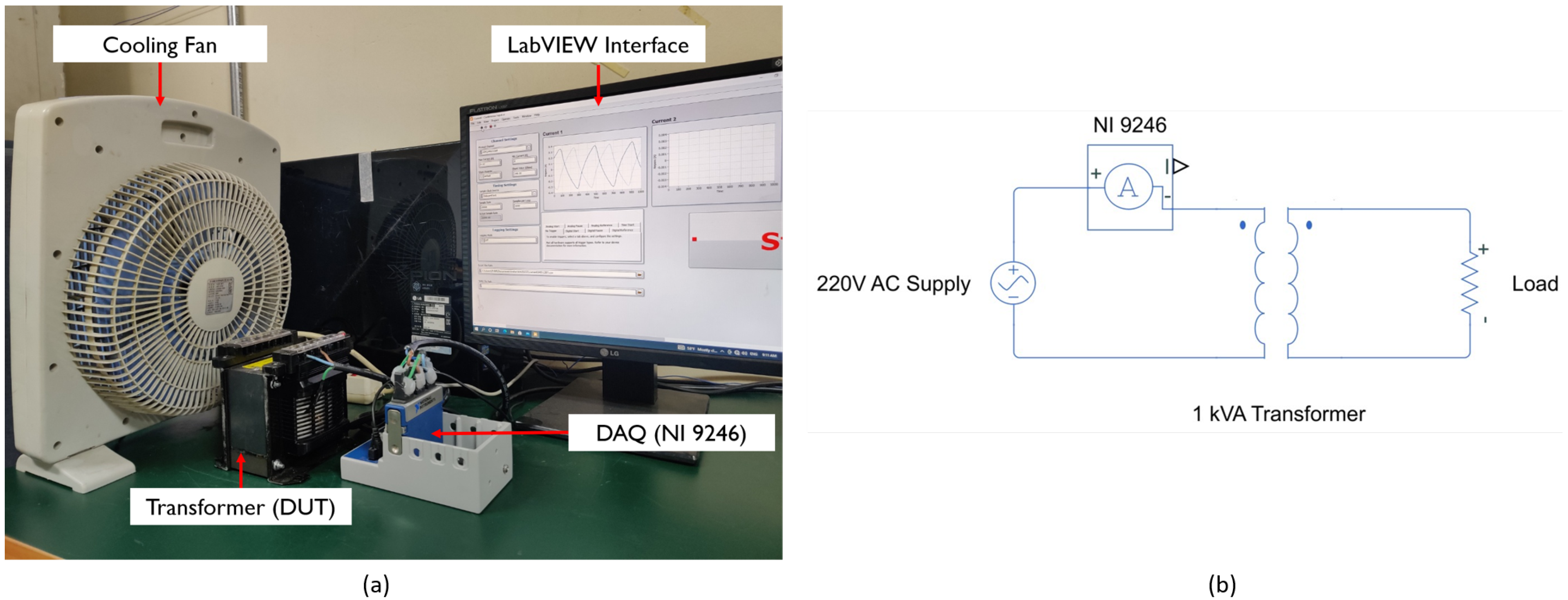
5. Experimental Setup and Data Collection

Figure 2a depicts the experimental test setup utilized to acquire the current signals. This setup was designed and executed at the Defense and Reliability Laboratory, Kumoh National Institute of Technology, Republic of Korea. The supply voltage was from a standard convenience outlet, featuring a rating of 220 V at a frequency of 60 Hz. Current measurements were conducted using the national instruments NI 9246 current module, seamlessly interfaced with LABVIEW software version 8.6.1 through the national instruments NI cDAQ-9174. The acquisition of current data occurred on the primary side of the circuit. Concurrently, on the secondary side, an electric fan was connected to function as a motor load for the transformer. The comprehensive circuit diagram is presented in Figure 2b. The NI 9246 specifications are listed as follows:

Figure 2. (a) Experimental testbed setup for transformer analysis. (b) Circuit diagram of the transformer core setup.

• Three isolated analog input channels were employed, each operating at a simultaneous sample rate of 50 kS/s, ensuring comprehensive data collection.
• The system offers a broad input range of 22 continuous arms, with a ±30 A peak input range and 24-bit resolution, exclusively for AC signals.
• Specifically designed to accommodate 1 A/5 A nominal CTs, ensuring compatibility and accuracy during measurements.
• Channel-to-earth isolation of up to 300 Vrms and channel-to-channel CAT III isolation of 480 Vrms guarantees safety and accuracy during experimentation.
• It has ring lug connectors tailored for up to 10 AWG cables, ensuring secure and reliable connections.
• It operates within a wide temperature range, from −40 °C to 70 °C, and is engineered to withstand 5 g vibrations and 50 g shocks, ensuring stability and functionality across varying environmental conditions.

In this study, we obtained three datasets representing different conditions of transformers: a healthy state (labeled as HLTY), a state with one hole in the core (labeled as 1HCF), and a state with two holes in the core (labeled as 2HCF). To simulate 1HCF, a 5 mm hole was drilled diagonally through the edge of the core. This was to replicate damage focused on the edge of the transformer. In the 2HCF, an additional 5 mm hole was drilled straight through the core from top to bottom, simulating core damage away from the edge of the transformer. Figure 3 illustrates the actual replication of these faults conducted during our experiment in the laboratory.

Figure 3. Actual faults induced: (a) 1HCF and (b) 2HCF.

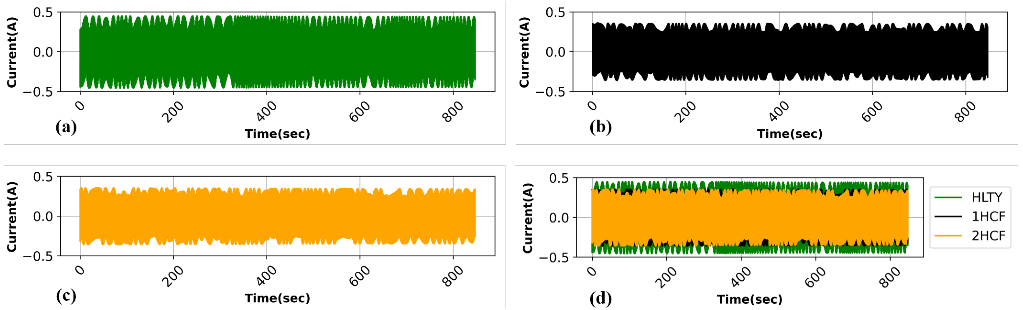
5.1. Applying Signal Processing Technique

In this study, we employed signal processing techniques to unveil crucial details within the signals that were obscured in the raw data. To assess the efficacy of our proposed model utilizing Hilbert transform (HT) on electric current data, we conducted a comparative analysis using fast Fourier transform (FFT) without employing any signal processing technique. Following the signal processing step, we applied a window size of 25 samples to the data before proceeding with statistical feature extraction.

Figure 4a–c display the electric current data obtained from the modules under three working conditions, HLTY, 1HCF, and 2HCF, represented by green, black, and orange. The data values range from −0.5 to 0.5 in all working conditions. During HLTY, the plot reveals that the maximum current in the circuit can reach −0.5 A to 0.5 A, with a notably cleaner waveform compared to other operating conditions. In the case of 1HCF, the current ranges from −0.4 A to 0.4 A, which is lower than the HLTY condition. The plot exhibits a random pattern with distortions in every cycle. Transitioning to 2HCF, the range of values is relatively similar to the 1HCF condition, varying from −0.4 A to 0.4 A. However, compared to HLTY, the waveform pattern differs. Upon close examination of each plot, it seems that using raw data could potentially aid in identifying core faults in transformers. However, upon closer examination in Figure 4d, which presents the plots for all working conditions, it becomes evident that there is no significant difference when comparing HLTY with the faulty conditions (1HCF and 2HCF). Figure 5 illustrates the FFT plots under various operating conditions, revealing the limitation of FFT in capturing essential changes across all scenarios. Upon observation, the plots in all conditions exhibit minimal variation, indicating that when features are extracted, there is a lack of discriminative information. Figure 6 demonstrates the substantial differences revealed after applying HT to the transformer core dataset, particularly distinguishing between healthy and faulty conditions. However, for the 1HCF and 2HCF plots, the differences may not be obvious, but the next section demonstrates a significant increase in the model’s performance. This observation underscores the effectiveness of our proposed signal processing technique’s usefulness in analyzing transformers’ core health based on current data. Identifying relevant characteristics and patterns in the raw signal proves to be pivotal in the initial stages of our methodology, as these factors significantly impact the overall performance of the ML model.

Figure 4. Plot of raw current signal: (a) HLTY, (b) 1HCF, (c) 2HCF, and (d) all working conditions.

Figure 5. FFT of all working conditions.

Figure 6. HT of all working conditions.

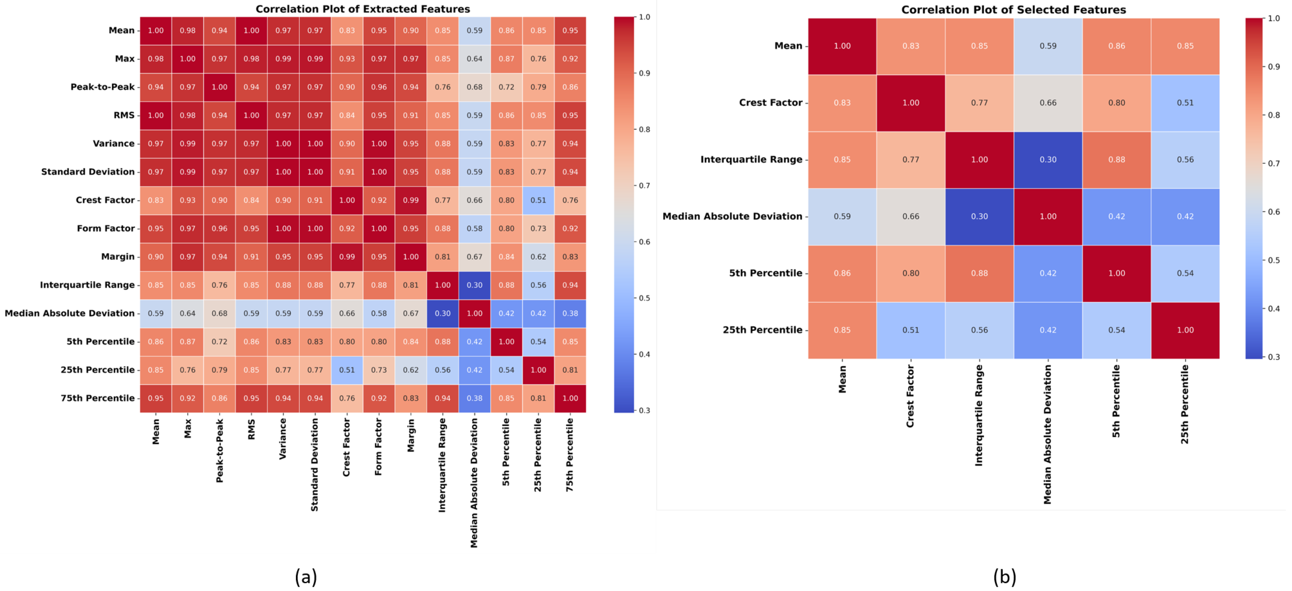
5.2. Correlation Matrix of Extracted and Selected Time-Domain Statistical Features

Figure 7a illustrates the correlation plot of the features extracted from the HT. The red intensity in the plot indicates the strength of the correlation among features, with a gradient from more red showing a stronger correlation to less red, and eventually blue, indicating a weaker correlation. This matrix visually represents the relationships between each feature, providing valuable insights for analysis and utilization. There is a notable correlation between the mean and other features, namely, max, peak-to-peak, RMS, variance, and standard deviation, with correlation coefficients of 0.98, 0.94, 1, 0.97, and 0.97, respectively. Recognizing such high correlations is crucial, as incorporating highly correlated features into the model can significantly and negatively impact its performance.

Figure 7. Statistical correlation matrix: (a) feature extraction and (b) feature selection.

Upon extracting features and generating the correlation matrix, it was evident that the features are highly correlated and could impact the model’s performance. To address this, we employed filter-based statistical feature selection. As illustrated in Figure 7b, out of the initially extracted 14 features, only 6 were retained, namely, mean, crest factor, interquartile range, median absolute deviation, 5th percentile, and 25th percentile, after eliminating those with high correlations. The resulting selected features were labeled with the values of 0, 1, and 2 and concatenated into a single data frame. This step further refined the dataset before feeding it into the ML model, enhancing its ability to capture relevant patterns and relationships in the data.

6. ML Diagnostic Results and Discussion

We need to split the dataset to train and test our model effectively. In our study, 80% of the dataset was allocated for training and 20% for testing, with a total size of 2541 samples. We used six established ML models: ABC, KNN, LR, MLP, SGD, and SVC. A summary of the parameters of the different models is presented in Table 4. The ML models highlight improvements under three conditions: raw data, FFT, and HT. The objective is to evaluate and compare the performance of these models in accurately classifying conditions such as HLTY, 1HCF, and 2HCF.

Table 4. Machine learning models and parameter values.

ML Model	Parameter	Value
AdaBoost (ABC)	n estimators	50
k-Nearest Neighbor (KNN)	k	9
Logistic Regression (LR)	Regularization	L2
Multilayer Perceptron (MLP)	Learning rate, n layers	Constant, 100
Stochastic Gradient Descent (SGD)	Loss function	Perceptron
Support Vector Machine (SVC)	C, gamma	90, scale

Our study’s significance lies in evaluating our proposed model’s performance thoroughly. By assessing the effectiveness of our method, we can validate its reliability and demonstrate its ability to identify and classify faults proactively. Ultimately, this will contribute to the overall reliability and efficiency of the transformer. In this study, we have employed classification metrics such as TP (true positive), FP (false positive), TN (true negative), and FN (false negative) to represent the counts of accurately predicted positive instances, inaccurately predicted positive instances, accurately predicted negative instances, and inaccurately predicted negative instances, respectively. We use these metrics along with their formulas and brief descriptions, as described in the references [51,52]:

Accuracy: Measures the overall correctness of the model.

$$\mathrm{Accuracy}=\frac{\mathrm{TP}+\mathrm{TN}}{\mathrm{TP}+\mathrm{FP}+\mathrm{TN}+\mathrm{FN}}$$

(7)

Precision: Indicates the accuracy of positive predictions.

$$\mathrm{Precision}=\frac{\mathrm{TP}}{\mathrm{TP}+\mathrm{FP}}$$

(8)

Recall: Emphasizes the model’s ability to capture all positive instances.

$$\mathrm{Recall}=\frac{\mathrm{TP}}{\mathrm{TP}+\mathrm{FN}}$$

(9)

F1 score: Provides a harmonic mean by balancing precision and recall. It is particularly valuable in scenarios with uneven class distribution.

$$\mathrm{F}1\mathrm{Score}=2·\frac{\mathrm{Precision}·\mathrm{Recall}}{\mathrm{Precision}+\mathrm{Recall}}$$

(10)

Table 5 presents a comprehensive evaluation of the machine learning model using raw data. LR (logistic regression) is identified as the top-performing model, with an accuracy of 65.23%. It shows the highest metrics, except for computational time, where KNN is the fastest with 0.0142 s. On the other hand, the lowest-performing model is SGD, with an accuracy of 29.08%. Generally, the machine learning models’ performance appears unsatisfactory when analyzing raw data, making them ineffective for detecting and classifying core faults.

Table 5. Performance evaluation for raw data.

ML Model	Accuracy (%)	Precision (%)	Recall (%)	F1 Score (%)	Time Cost (s)
ABC	59.39	56.38	56.39	56.37	0.3425
KNN	37.72	41.35	37.72	38.84	0.1421
LR	65.23	65.13	65.23	64.94	0.0427
MLP	48.33	47.53	48.33	47.85	0.1745
SGD	29.08	19.51	29.08	23.34	0.0170
SVC	32.81	16.68	32.81	17.36	0.2040

To truly understand the effectiveness of a model, it is crucial to incorporate frequency-domain analysis, mainly using FFT. The resulting comprehensive and insightful perspective provides a detailed comparative analysis that sheds light on the model’s performance. Table 6 presents a comprehensive evaluation of the machine learning model with FFT signal processing. The data shows that ABC performs the best among all models, with an accuracy of 61.49%, demonstrating superior performance in all aspects. Meanwhile, KNN delivers the fastest computational time, making it a noteworthy contender. However, the SVC model struggles, with an accuracy of only 33.20%. Despite these findings, it is worth noting that the overall performance of the ML models remain low in frequency-domain analyses, which limits their effectiveness in detecting and classifying core faults.

Table 6. Performance evaluation for FFT.

ML Model	Accuracy (%)	Precision (%)	Recall (%)	F1 Score (%)	Time Cost (s)
ABC	61.49	60.88	61.49	60.74	0.2545
KNN	54.22	55.63	54.22	54.63	0.0138
LR	33.40	24.37	33.40	25.88	0.0168
MLP	43.61	29.73	43.61	35.06	0.1381
SGD	33.40	24.37	33.40	25.88	0.0156
SVC	33.20	30.89	33.20	18.74	0.1980

The ML model performance metrics presented in Table 7 provide compelling evidence of the superior performance of the KNN model, which boasts the highest values across all parameters, an accuracy of 83.89%, and a remarkable computational time of 0.0156 s. Our proposed method, utilizing HT and Pearson correlation filter-based feature selection, enhances the performance across all metrics in the ML models, except for time cost, as shown in Figure 8. This compelling figure substantiates the effectiveness of our model, which outperforms all ML models when diagnosing and classifying core faults. The confusion matrix, depicted in Figure 9, provides consistent improvements in TP and a reduction in FP, with the ABC and SGD models predicting the highest number of FP instances (121 and 171, respectively). Conversely, other models demonstrated an increase in TP predictions, evident from the values along the diagonal. Our model’s notable enhancement in performance when employing the HT for analyses makes it a compelling choice for any team looking to improve the efficiency and accuracy of core fault diagnosis and classification.

Table 7. Performance evaluation for HT.

ML Model	Accuracy (%)	Precision (%)	Recall (%)	F1 Score (%)	Time Cost (s)
ABC	66.60	66.42	66.60	64.95	0.2963
KNN	83.89	84.39	83.89	83.79	0.0156
LR	71.91	72.16	71.91	72.01	0.0251
MLP	73.45	73.51	73.48	73.47	1.3454
SGD	66.01	46.66	66.01	54.99	0.0253
SVC	72.10	72.11	72.10	72.10	0.0732

Figure 8. Plot of ML models’ performance evaluation under three conditions: using raw data, using FFT, and using HT.

Figure 9. Confusion matrix of ML models via Hilbert transform signal processing from the test data. (a) ABC, (b) SGD, (c), LR, (d) SVC, (e) MLP, and (f) KNN.

Limitations, Open Issues, and Future Directions

This study integrates signal processing with filter-based Pearson correlation feature selection, employing FFT and HT. Our reliance on comparative analysis between signal processing techniques, such as the HT (proposed), and frequency-domain analysis, notably the FFT, using only raw data, provides valuable insights into their respective efficacy. We acknowledge the limitations of utilizing the HT for fault classification compared to deep learning methodologies. While our study demonstrates the effectiveness of the HT in analyzing current signals and characterizing fault signatures in a single-phase transformer core, it is essential to recognize its inherent constraints. Firstly, the performance of the HT may be influenced by signal noise and variability, particularly in real-world applications, where environmental factors and measurement inaccuracies can impact signal quality. It may reduce the robustness and reliability of fault classification outcomes, potentially leading to misdiagnosis or false alarms [53]. Secondly, the HT’s effectiveness in capturing complex nonlinear relationships and subtle fault patterns may be limited compared to deep learning methodologies. Deep learning algorithms, such as convolutional neural networks (CNNs) and recurrent neural networks (RNNs), excel in learning intricate features and hierarchical representations from raw data, enabling more nuanced fault classification capabilities [54]. Additionally, the reliance on handcrafted features and manual feature selection in HT-based approaches may pose challenges in capturing and leveraging all relevant information in the data. On the other hand, deep learning models can automatically extract discriminative features from raw signals, minimizing the need for manual intervention and potentially enhancing diagnostic accuracy. Furthermore, the scalability and generalizability of HT-based fault classification methods may be limited when faced with diverse fault scenarios or variations in transformer operating conditions. With their adaptability and ability to learn from large and varied datasets, deep learning methodologies offer more significant potential for robust performance across various operating conditions and fault types [55]. Moreover, the potential for overfitting in deep learning models should be considered, as it can lead to poor generalization and decreased performance on unseen data. Adequate regularization techniques must be employed to mitigate this risk and ensure the reliability of fault classification results [56,57,58]. In scenarios where deep learning models may not be feasible, the HT provides a pragmatic alternative that can yield valuable insights into the system’s health. Its simplicity and efficiency make it particularly attractive for real-time or resource-constrained environments, where complex modeling approaches may need to be more practical [59,60]. Furthermore, the HT’s transparent and intuitive nature facilitates straightforward interpretation of results, making it accessible to a broader range of practitioners without extensive expertise in machine learning or data science. It can be advantageous in fields where practicality and ease of implementation are paramount. Overall, while deep learning models offer potent capabilities for fault diagnosis, the HT approach remains relevant in situations where practical considerations necessitate a more straightforward, accessible solution. It is not a question of one approach being superior to the other but instead selecting the most appropriate method based on the specific requirements and constraints of the application.

7. Conclusions

This study presents the application of HT as a signal processing technique, utilizing a Pearson correlation-based statistical feature approach for classifying the condition of a transformer’s core. The study evaluates the performance of various machine learning models on the transformer core current dataset collected during healthy and faulty conditions. The proposed method is compared under two scenarios: without any signal processing technique and when applying FFT. The results illustrate an improvement in the performance of six ML models, as evidenced by their performance metrics. Our current dataset can serve as a reference for future research on monitoring the transformer’s core. For future works, we will look at improving the proposed model’s accuracy and effectiveness with deep learning algorithms and vibration signal acquisition.

References

1. Kim, N.H.; An, D.; Choi, J.H. Prognostics and Health Management of Engineering Systems: An Introduction; Springer: Cham, Switzerland, 2017; pp. 127–241. [Google Scholar]
2. Do, J.S.; Kareem, A.B.; Hur, J.-W. LSTM-Autoencoder for Vibration Anomaly Detection in Vertical Carousel Storage and Retrieval System (VCSRS). Sensors 2023, 23, 1009. [Google Scholar] [CrossRef]
3. Fink, O.; Wang, Q.; Svensén, M.; Dersin, P.; Lee, W.-J.; Ducoffe, M. Potential, challenges and future directions for deep learning in prognostics and health management applications. Eng. Appl. Artif. Intell. 2020, 92, 103678. [Google Scholar] [CrossRef]
4. Jia, Z.; Wang, S.; Zhao, K.; Li, Z.; Yang, Q.; Liu, Z. An efficient diagnostic strategy for intermittent faults in electronic circuit systems by enhancing and locating local features of faults. Meas. Sci. Technol. 2024, 35, 036107. [Google Scholar] [CrossRef]
5. Aciu, A.-M.; Nițu, M.-C.; Nicola, C.-I.; Nicola, M. Determining the Remaining Functional Life of Power Transformers Using Multiple Methods of Diagnosing the Operating Condition Based on SVM Classification Algorithms. Machines 2024, 12, 37. [Google Scholar] [CrossRef]
6. Yu, Q.; Bangalore, P.; Fogelström, S.; Sagitov, S. Optimal Preventive Maintenance Scheduling for Wind Turbines under Condition Monitoring. Energies 2024, 17, 280. [Google Scholar] [CrossRef]
7. Zhuang, L.; Johnson, B.K.; Chen, X.; William, E. A topology-based model for two-winding, shell-type, single-phase transformer inter-turn faults. In Proceedings of the 2016 IEEE/PES Trans. and Dist. Conference and Exposition (T&D), Dallas, TX, USA, 3–5 May 2016; pp. 1–5. [Google Scholar]
8. Manohar, S.S.; Subramaniam, A.; Bagheri, M.; Nadarajan, S.; Gupta, A.K.; Panda, S.K. Transformer Winding Fault Diagnosis by Vibration Monitoring. In Proceedings of the 2018 Condition Monitoring and Diagnosis (CMD), Perth, WA, Australia, 23–26 September 2018; pp. 1–6. [Google Scholar]
9. Olayiwola, T.N.; Hyun, S.-H.; Choi, S.-J. Photovoltaic Modeling: A Comprehensive Analysis of the I–V Characteristic Curve. Sustainability 2024, 16, 432. [Google Scholar] [CrossRef]
10. Islam, M.M.; Lee, G.; Hettiwatte, S.N. A nearest neighbor clustering approach for incipient fault diagnosis of power transformers. Electr. Eng. 2017, 99, 1109–1119. [Google Scholar] [CrossRef]
11. Wang, M.; Vandermaar, A.J.; Srivastava, K.D. Review of condition assessment of power transformers in service. IEEE Electr. Insul. Mag. 2002, 18, 12–25. [Google Scholar] [CrossRef]
12. Okwuosa, C.N.; Hur, J.W. A Filter-Based Feature-Engineering-Assisted SVC Fault Classification for SCIM at Minor-Load Conditions. Energies 2022, 15, 7597. [Google Scholar] [CrossRef]
13. Kareem, A.B.; Hur, J.-W. Towards Data-Driven Fault Diagnostics Framework for SMPS-AEC Using Supervised Learning Algorithms. Electronics 2022, 11, 2492. [Google Scholar] [CrossRef]
14. Shifat, T.A.; Hur, J.W. ANN Assisted Multi-Sensor Information Fusion for BLDC Motor Fault Diagnosis. IEEE Access 2021, 9, 9429–9441. [Google Scholar] [CrossRef]
15. Lee, J.-H.; Okwuosa, C.N.; Hur, J.-W. Extruder Machine Gear Fault Detection Using Autoencoder LSTM via Sensor Fusion Approach. Inventions 2023, 8, 140. [Google Scholar] [CrossRef]
16. Kareem, A.B.; Hur, J.-W. A Feature Engineering-Assisted CM Technology for SMPS Output Aluminium Electrolytic Capacitors (AEC) Considering D-ESR-Q-Z Parameters. Processes 2022, 10, 1091. [Google Scholar] [CrossRef]
17. Gao, B.; Yu, R.; Hu, G.; Liu, C.; Zhuang, X.; Zhou, P. Development Processes of Surface Trucking and Partial Discharge of Pressboards Immersed in Mineral Oil: Effect of Tip Curvatures. Energies 2019, 12, 554. [Google Scholar] [CrossRef]
18. Liu, J.; Cao, Z.; Fan, X.; Zhang, H.; Geng, C.; Zhang, Y. Influence of Oil–Pressboard Mass Ratio on the Equilibrium Characteristics of Furfural under Oil Replacement Conditions. Polymers 2020, 12, 2760. [Google Scholar] [CrossRef]
19. Fritsch, M.; Wolter, M. Saturation of High-Frequency Current Transformers: Challenges and Solutions. IEEE Trans. Instrum. Meas. 2023, 72, 9004110. [Google Scholar] [CrossRef]
20. Altayef, E.; Anayi, F.; Packianather, M.; Benmahamed, Y.; Kherif, O. Detection and Classification of Lamination Faults in a 15 kVA Three-Phase Transformer Core Using SVM, KNN and DT Algorithms. IEEE Access 2022, 10, 50925–50932. [Google Scholar] [CrossRef]
21. Yuan, F.; Shang, Y.; Yang, D.; Gao, J.; Han, Y.; Wu, J. Comparison on multiple signal analysis method in transformer core looseness fault. In Proceedings of the IEEE Asia-Pacific Conference on Image Processing, Electronics and Computers, Dalian, China, 14–16 April 2021. [Google Scholar]
22. Tian, H.; Peng, W.; Hu, M.; Yuan, G.; Chen, Y. Feature extraction of the transformer core loosening based on variational mode decomposition. In Proceedings of the 2017 1st International Conference on Electrical Materials and Power Equipment (ICEMPE), Xi’an, China, 14–17 May 2017. [Google Scholar]
23. Yao, D.; Li, L.; Zhang, S.; Zhang, D.; Chen, D. The Vibroacoustic Characteristics Analysis of Transformer Core Faults Based on Multi-Physical Field Coupling. Symmetry 2022, 14, 544. [Google Scholar] [CrossRef]
24. Bagheri, M.; Zollanvari, A.; Nezhivenko, S. Transformer Fault Condition Prognosis Using Vibration Signals Over Cloud Environment. IEEE Access 2018, 6, 9862–9874. [Google Scholar] [CrossRef]
25. Shengchang, J.; Yongfen, L.; Yanming, L. Research on extraction technique of transformer core fundamental frequency vibration based on OLCM. IEEE Trans. Power Deliv. 2006, 21, 1981–1988. [Google Scholar] [CrossRef]
26. Okwuosa, C.N.; Hur, J.W. An Intelligent Hybrid Feature Selection Approach for SCIM Inter-Turn Fault Classification at Minor Load Conditions Using Supervised Learning. IEEE Access 2023, 11, 89907–89920. [Google Scholar] [CrossRef]
27. Pietrzak, P.; Wolkiewicz, M. Demagnetization Fault Diagnosis of Permanent Magnet Synchronous Motors Based on Stator Current Signal Processing and Machine Learning Algorithms. Sensors 2023, 23, 1757. [Google Scholar] [CrossRef]
28. Merizalde, Y.; Hernández-Callejo, L.; Duque-Perez, O.; López-Meraz, R.A. Fault Detection of Wind Turbine Induction Generators through Current Signals and Various Signal Processing Techniques. Appl. Sci. 2020, 10, 7389. [Google Scholar] [CrossRef]
29. Dehina, W.; Boumehraz, M.; Kratz, F. Detectability of rotor failure for induction motors through stator current based on advanced signal processing approaches. Int. J. Dynam. Control 2021, 9, 1381–1395. [Google Scholar] [CrossRef]
30. Pradhan, P.K.; Roy, S.K.; Mohanty, A.R. Detection of Broken Impeller in Submersible Pump by Estimation Rotational Frequency from Motor Current Signal. J. Vib. Eng. Technol. 2020, 8, 613–620. [Google Scholar] [CrossRef]
31. Zhao, K.; Liu, Z.; Zhao, B.; Shao, H. Class-Aware Adversarial Multiwavelet Convolutional Neural Network for Cross-Domain Fault Diagnosis. IEEE Trans. Ind. Inform. 2023, 1–12. [Google Scholar] [CrossRef]
32. Altaf, M.; Akram, T.; Khan, M.A.; Iqbal, M.; Ch, M.M.I.; Hsu, C.-H. A New Statistical Features Based Approach for Bearing Fault Diagnosis Using Vibration Signals. Sensors 2022, 22, 2012. [Google Scholar] [CrossRef] [PubMed]
33. Akpudo, U.E.; Hur, J.-W. A Cost-Efficient MFCC-Based Fault Detection and Isolation Technology for Electromagnetic Pumps. Electronics 2021, 10, 439. [Google Scholar] [CrossRef]
34. Badihi, H.; Zhang, Y.; Jiang, B.; Pillay, P.; Rakheja, S. A Comprehensive Review on Signal-Based and Model-Based Condition Monitoring of Wind Turbines: Fault Diagnosis and Lifetime Prognosis. Proc. IEEE 2022, 110, 754–806. [Google Scholar] [CrossRef]
35. Ismail, A.; Saidi, L.; Sayadi, M.; Benbouzid, M. A New Data-Driven Approach for Power IGBT Remaining Useful Life Estimation Based On Feature Reduction Technique and Neural Network. Electronics 2018, 9, 1571. [Google Scholar] [CrossRef]
36. Stavropoulos, G.; van Vorstenbosch, R.; van Schooten, F.; Smolinska, A. Random Forest and Ensemble Methods. Chemom. Chem. Biochem. Data Anal. 2020, 2, 661–672. [Google Scholar]
37. Yang, J.; Sun, Z.; Chen, Y. Fault Detection Using the Clustering-kNN Rule for Gas Sensor Arrays. Sensors 2016, 16, 2069. [Google Scholar] [CrossRef] [PubMed]
38. Wang, X.; Jiang, Z.; Yu, D. An Improved KNN Algorithm Based on Kernel Methods and Attribute Reduction. In Proceedings of the 5th International Conference on Instrumentation and Measurement, Computer, Communication and Control (IMCCC), Qinhuangdao, China, 18–20 September 2015; pp. 567–570. [Google Scholar]
39. Saadatfar, H.; Khosravi, S.; Joloudari, J.H.; Mosavi, A.; Shamshirband, S. A New K-Nearest Neighbors Classifier for Big Data Based on Efficient Data Pruning. Mathematics 2020, 8, 286. [Google Scholar] [CrossRef]
40. Couronné, R.; Probst, P.; Boulesteix, A.-L. Random forest versus logistic regression: A large-scale benchmark experiment. BMC Bioinform. 2018, 19, 270. [Google Scholar] [CrossRef] [PubMed]
41. Carreras, J.; Kikuti, Y.Y.; Miyaoka, M.; Hiraiwa, S.; Tomita, S.; Ikoma, H.; Kondo, Y.; Ito, A.; Nakamura, N.; Hamoudi, R. A Combination of Multilayer Perceptron, Radial Basis Function Artificial Neural Networks and Machine Learning Image Segmentation for the Dimension Reduction and the Prognosis Assessment of Diffuse Large B-Cell Lymphoma. AI 2021, 2, 106–134. [Google Scholar] [CrossRef]
42. Huang, J.; Ling, S.; Wu, X.; Deng, R. GIS-Based Comparative Study of the Bayesian Network, Decision Table, Radial Basis Function Network and Stochastic Gradient Descent for the Spatial Prediction of Landslide Susceptibility. Land 2022, 11, 436. [Google Scholar] [CrossRef]
43. Han, T.; Jiang, D.; Zhao, Q.; Wang, L.; Yin, K. Comparison of random forest, artificial neural networks and support vector machine for intelligent diagnosis of rotating machinery. Trans. Inst. Meas. Control 2018, 40, 2681–2693. [Google Scholar] [CrossRef]
44. Riza Alvy Syafi’i, M.H.; Prasetyono, E.; Khafidli, M.K.; Anggriawan, D.O.; Tjahjono, A. Real Time Series DC Arc Fault Detection Based on Fast Fourier Transform. In Proceedings of the 2018 International Electronics Symposium on Engineering Technology and Applications (IES-ETA), Bali, Indonesia, 29–30 October 2018; pp. 25–30. [Google Scholar]
45. Misra, S.; Kumar, S.; Sayyad, S.; Bongale, A.; Jadhav, P.; Kotecha, K.; Abraham, A.; Gabralla, L.A. Fault Detection in Induction Motor Using Time Domain and Spectral Imaging-Based Transfer Learning Approach on Vibration Data. Sensors 2022, 22, 8210. [Google Scholar] [CrossRef]
46. Ewert, P.; Kowalski, C.T.; Jaworski, M. Comparison of the Effectiveness of Selected Vibration Signal Analysis Methods in the Rotor Unbalance Detection of PMSM Drive System. Electronics 2022, 11, 1748. [Google Scholar] [CrossRef]
47. El Idrissi, A.; Derouich, A.; Mahfoud, S.; El Ouanjli, N.; Chantoufi, A.; Al-Sumaiti, A.S.; Mossa, M.A. Bearing fault diagnosis for an induction motor controlled by an artificial neural network—Direct torque control using the Hilbert transform. Mathematics 2022, 10, 4258. [Google Scholar] [CrossRef]
48. Dias, C.G.; Silva, L.C. Induction Motor Speed Estimation based on Airgap flux measurement using Hilbert transform and fast Fourier transform. IEEE Sens. J. 2022, 22, 12690–12699. [Google Scholar] [CrossRef]
49. Metsämuuronen, J. Artificial systematic attenuation in eta squared and some related consequences: Attenuation-corrected eta and eta squared, negative values of eta, and their relation to Pearson correlation. Behaviormetrika 2023, 50, 27–61. [Google Scholar] [CrossRef]
50. Denuit, M.; Trufin, J. Model selection with Pearson’s correlation, concentration and Lorenz curves under autocalibration. Eur. Actuar. J. 2023, 13, 871–878. [Google Scholar] [CrossRef]
51. Kareem, A.B.; Ejike Akpudo, U.; Hur, J.-W. An Integrated Cost-Aware Dual Monitoring Framework for SMPS Switching Device Diagnosis. Electronics 2021, 10, 2487. [Google Scholar] [CrossRef]
52. Jeong, S.; Kareem, A.B.; Song, S.; Hur, J.-W. ANN-Based Reliability Enhancement of SMPS Aluminum Electrolytic Capacitors in Cold Environments. Energies 2023, 16, 6096. [Google Scholar] [CrossRef]
53. Satija, U.; Ramkumar, B.; Manikandan, M.S. A Review of Signal Processing Techniques for Electrocardiogram Signal Quality Assessment. IEEE Rev. Biomed. Eng. 2018, 11, 36–52. [Google Scholar] [CrossRef] [PubMed]
54. Qiu, S.; Cui, X.; Ping, Z.; Shan, N.; Li, Z.; Bao, X.; Xu, X. Deep Learning Techniques in Intelligent Fault Diagnosis and Prognosis for Industrial Systems: A Review. Sensors 2023, 23, 1305. [Google Scholar] [CrossRef] [PubMed]
55. Hakim, M.; Omran, A.; Ahmed, A.; Al-Waily, M.; Abdellatif, A. A systematic review of rolling bearing fault diagnoses based on deep learning and transfer learning: Taxonomy, overview, application, open challenges, weaknesses and recommendations. Ain Shams Eng. J. 2023, 14, 101945. [Google Scholar] [CrossRef]
56. Ying, X. An Overview of Overfitting and its Solutions. J. Phys. Conf. Ser. 2019, 1168, 022022. [Google Scholar] [CrossRef]
57. Alzubaidi, L.; Zhang, J.; Humaidi, A.J.; Al-Dujaili, A.; Duan, Y.; Al-Shamma, O.; Santamaría, J.; Fadhel, M.A.; Al-Amidie, M.; Farhan, L. Review of deep learning: Concepts, CNN architectures, challenges, applications, future directions. J. Big Data 2021, 8, 53. [Google Scholar] [CrossRef] [PubMed]
58. Rahman, K.; Ghani, A.; Misra, S.; Rahman, A.U. A deep learning framework for non-functional requirement classification. Sci. Rep. 2024, 14, 3216. [Google Scholar] [CrossRef] [PubMed]
59. Taye, M.M. Understanding of Machine Learning with Deep Learning: Architectures, Workflow, Applications and Future Directions. Computers 2023, 12, 91. [Google Scholar] [CrossRef]
60. Sarker, I.H. Deep Learning: A Comprehensive Overview on Techniques, Taxonomy, Applications and Research Directions. SN Comput. Sci. 2021, 2, 420. [Google Scholar] [CrossRef] [PubMed]
Disclaimer/Publisher’s Note: The statements, opinions and data contained in all publications are solely those of the individual author(s) and contributor(s) and not of MDPI and/or the editor(s). MDPI and/or the editor(s) disclaim responsibility for any injury to people or property resulting from any ideas, methods, instructions or products referred to in the content.
Article Metrics
Citations
Article Access Statistics
Multiple requests from the same IP address are counted as one view.