DiffQuant: Reducing Compression Difference for Neural Network Quantization

Abstract

Deep neural network quantization is a widely used method in the deployment of mobile or edge devices to effectively reduce memory overhead and speed up inference. However, quantization inevitably leads to a reduction in the performance and equivalence of models. Moreover, access to labeled datasets is often denied as they are considered valuable assets for companies or institutes. Consequently, performing quantization training becomes challenging without sufficient labeled datasets. To address these issues, we propose a novel quantization pipeline named DiffQuant, which can perform quantization training using unlabeled datasets. The pipeline includes two cores: the compression difference (CD) and model compression loss (MCL). The CD can measure the degree of equivalence loss between the full-precision and quantized models, and the MCL supports fine-tuning the quantized models using unlabeled data. In addition, we design a quantization training scheme that allows the quantization of both the batch normalization (BN) layer and the bias. Experimental results show that our method outperforms state-of-the-art methods on ResNet18/34/50 networks, maintaining performance with a reduced CD. We achieve Top-1 accuracies of 70.08%, 74.11%, and 76.16% on the ImageNet dataset for the 8-bit quantized ResNet18/34/50 models and reduce the gap to 0.55%, 0.61%, and 0.71% with the full-precision network, respectively. We achieve CD values of only 7.45%, 7.48%, and 8.52%, which allows DiffQuant to further exploit the potential of quantization.

1. Introduction

Deep convolutional networks (DCNs) have been widely used in object detection [1,2], image classification [3,4], incremental learning [5], and semantic segmentation [6]. However, deploying DCNs on resource-limited mobile or edge devices remains challenging owing to their dense parameters and the multitude of multiply-accumulate (MAC) operations they require. To address these issues, scholars have proposed various techniques, such as knowledge distillation [7], pruning [8], and network quantization [9]. Quantization is a popular and effective method for improving memory utilization and inference speed. However, quantization can cause performance degradation as the bit width decreases. Studies [10,11] have focused on maintaining high accuracy while quantizing at lower bit widths. Preserving the first and last layers of networks without quantization or using a higher bit width can lead to better performance [12,13]. Uniform quantization maintains the same bit width across all layers, which facilitates hardware design and deployment [14,15,16,17,18]. Recent studies have utilized neural network search (NAS) [19,20,21,22,23,24,25] and mixed-precision quantization [26,27,28,29] for further optimization. However, quantization training methods like quantization-aware training [30] require the use of labeled datasets to fine-tune quantized weights based on the loss between dataset labels and model predictions. Therefore, it becomes impractical in the absence of labeled data. Companies or institutes often request the quantization of network models without providing labeled datasets. The provision of labeled datasets may pose a risk to the property of the company. This is because labeling datasets requires significant human, material, and financial resources from the company. Conversely, unlabeled datasets may be abundant and easier to supply. Some novel algorithms explore data-free quantization schemes [31,32,33,34], which construct simulated data for quantization through internal parameters (weights, biases, etc., of the convolution, BN, and linear layers of a model) of the original models. However, it is difficult for such schemes to enable quantized models to learn the data distribution pattern of real datasets, thereby reducing performance. Moreover, the equivalence loss between the quantized and original models is always ignored [35]. In conventional quantization training methods, the loss is computed using the output of the quantized model and the dataset labels, and the weights are fine-tuned in a backward process. This quantization approach sometimes does not lead to a decrease in model performance and may even result in improvements. However, it leads to a reduction in the similarity between the quantized and full-precision models, i.e., a decrease in the equivalence. The equivalence refers to the situation where the quantized model incorrectly predicts results that the full-precision model correctly predicts, and vice versa, despite exhibiting comparable performance to the full-precision model. Therefore, we find that exploring the enhancement of quantized model performance from the perspective of reducing the equivalence loss is a promising approach to quantization. It provides a better understanding of the process by which quantization leads to a decrease in model performance. Additionally, reducing the compression loss between both models has a positive impact on helping quantized models approach or surpass the accuracy of the floating-point model. The floating-point model is a full-precision model in which both the storage of model parameters and the computation of the model are carried out using floating-point numbers. To address these issues, we hope to fine-tune the quantized model using unlabeled datasets, thereby improving its performance by reducing the compression loss. We introduce a novel loss function that adjusts the parameters of the quantized models. We design a metric to measure the equivalence between full-precision and quantized models. In addition, we design a quantization training scheme that allows the quantization of both the batch normalization (BN) layer and the bias.

The contributions of this work are as follows:

• We propose the use of the model compression loss (MCL) function for training the quantized model, thereby improving accuracy by reducing the compression difference (CD) while maintaining equivalence between both models.
• We design a quantization training pipeline named DiffQuant, which can fine-tune quantized models using only unlabeled datasets and better support the quantization of both the batch normalization (BN) layer and the bias.
• We evaluate the proposed method for various networks and achieve good results on the CIFAR-100 and ImageNet datasets.

The rest of this paper is structured as follows. Section 2 analyzes the deficiencies of commonly used loss functions and introduces the current uniform quantization algorithms for general DCNs. Section 3 proposes the MCL function for better quantization when fine-tuning models and the quantization algorithm, which supports the quantization of the bias and batch normalization and simulates the inference on hardware. Section 4 describes a series of experiments on the public datasets CIFAR-10/100 and ImageNet to validate the effectiveness of the proposed method. Section 5 concludes our study and highlights the focus of further research.

2. Preliminaries

We first introduce the background of the loss functions and discuss the limitations of the commonly employed methods. We then discuss uniform quantization schemes and apply them to enhance the effectiveness of our design. Finally, we introduce the method for quantizing parameters in batch normalization.

2.1. Loss Function

Loss functions play a critical role in measuring the disparities between a model’s output and labels when optimizing parameters during the training phase. The mean-squared error (MSE) and cross-entropy (CE) are commonly used loss functions. However, these functions, which gauge the model’s output and labels, fail to account for potential discrepancies between the floating-point and quantized models, often resulting in unexpected errors. For example, we trained the LeNet model using the CE loss function based on the output of the floating-point model and the labels, achieving an accuracy of up to 82.07% on the CIFAR-10 dataset. After quantization, the model exhibited discrepancies when training using the identical loss function. Figure 1a,b illustrate confusion matrices of the floating-point and quantized models, where the bluer the color, the more samples there are.

Upon initial inspection, Figure 1a resembles Figure 1b, but they differ in their values. To better illustrate this discrepancy, we computed the absolute value of the difference between the floating-point and quantized models, as shown in Figure 1c. Despite achieving an accuracy of 81.60%, which only represents a decrease of 0.47%, the quantized model deviated from the floating-point model by 1.11% because it correctly classified an additional 32 samples (0.32%) compared to the floating-point model but misclassified 79 samples (0.79%).

Although the quantized model has lower bit-width parameters and maintains accuracy relative to the floating-point model, its resemblance to the original model has diminished. This could be even more pronounced in situations with stricter standards for quantized models. For instance, it is challenging to ensure consistency in recognition results between quantized and floating-point models when using identical input data while maintaining overall sample classification correctness. Therefore, we propose a novel criterion to address this issue, which is discussed in Section 3.1.

2.2. Uniform Quantization Schemes

Uniform quantizers have received significant attention in recent years because they enable MAC operations in the integer domain and facilitate high-throughput pipelines. The uniform quantizer can be divided into two styles: affine quantization and scale quantization, which are illustrated in Figure 2.

The first step of the uniform quantizer is to choose a range in which the real numbers will be quantized, clipping any values that fall outside this range. Then, the real values are mapped to an integer representation with the desired bit width by rounding each real number to the closest integer value within the range.

For affine quantization, the transformation function is given by:

$$\begin{array}{c}\hfill s=\frac{2^N-1}{b-a}=\frac{2^N-1}{max\left(\mathit{X}\right)-min\left(\mathit{X}\right)}\end{array}$$

(1)

$$\begin{array}{c}\hfill z=-\mathrm{round}\left(a·s\right)-2^{N-1}\end{array}$$

(2)

where N is the bit width, s is the scale factor, $[a,b]$ is the coverage that preserves the range of real numbers, $\mathit{X}$ is the real dataset, z is the value of zero shift, and round(·) rounds real values to the nearest integer values. With these parameters, a real number $x\in \mathbb{R},x\in \mathit{X}$ can be quantized to $\widehat{x}$ using Equation (3), in which $\widehat{x}$ is a pseudo-value that represents the quantized value (integer) using a real number type (floating point).

$$\begin{array}{c}\hfill \widehat{x}=\frac{1}{s}\left(x_q-z\right)\end{array}$$

(3)

Here, $x_q$ is the quantized integer obtained by:

$$\begin{array}{c}\hfill x_{s,z}=\mathrm{round}\left(s·x+z\right)\end{array}$$

(4)

$$\begin{array}{cc}\hfill x_q& =\mathrm{quantize}\left(N,x_{s,z}\right)\hfill \\ \hfill & =\mathrm{clip}\left(x_{s,z},-2^{N-1},2^{N-1}-1\right)\hfill \\ \hfill & =\left\{\begin{array}{c}-2^{N-1},x_{s,z}<-2^{N-1}\hfill \\ x_{s,z},-2^{N-1}<x_{s,z}<2^{N-1}-1\hfill \\ 2^{N-1}-1,x_{s,z}>2^{N-1}-1\hfill \end{array}\right.\hfill \end{array}$$

(5)

where $x_{s,z}$ is the integer after scaling, and clip(·) clips the integer, preventing values from beyond the range of the bit width. As a result, $x_q\in \left[-2^{N-1},-2^{N-1}+1,\cdots ,2^{N-1}-1\right]$. Equation (3) is often regarded as a dequantization that transforms a quantized number into a real number.

For scale quantization (often called symmetric quantization), the range of real and integer numbers is symmetric around zero. Unlike affine quantization, zero shift is not needed in scale quantization, whose transformation function is shown in Equations (6)–(8):

$$\begin{array}{c}\hfill s=\frac{2^{N-1}-1}{max\left(\left|\mathit{X}\right|\right)}\end{array}$$

(6)

$$\begin{array}{c}\hfill x_{s,z}=\mathrm{round}\left(s·x\right)\end{array}$$

(7)

$$\begin{array}{c}\hfill \widehat{x}=\frac{1}{s}·\mathrm{quantize}\left(N,x_{s,z}\right)\end{array}$$

(8)

2.3. Batch Normalization

In most convolutional neural networks, batch normalization appears frequently because of its flexibility and effectiveness in preventing models from overfitting and gradient exploration, as well as accelerating convergence. Batch normalization contains two learnable parameters that can reduce the internal covariate shift, given by:

$$\begin{array}{c}{y}_i=\mathrm{BN}\left(x_i\right)=\left(\frac{x_i-\mu }{\sqrt{{\sigma }^2+ϵ}}\right)·\gamma +\beta \end{array}$$

(9)

Here, $x_i$ and $y_i$ are the input and output data of a mini-batch in batch normalization, respectively. $\mu$ and $\sigma$ are the mean and variance of $x_i$, respectively, which normalize the distribution of $x_i$ to $N(0,1)$. $\gamma$ and $\beta$ are learnable parameters used for introducing transformation and reconstruction, respectively, both of which significantly enhance the layer’s representational capacity. $ϵ$ is a small positive number that prevents the denominator from becoming zero.

For the quantization of batch normalization, there is a simple method that fuses the four parameters into two and absorbs the fused parameters into adjacent computing layers:

$$\begin{array}{cc}\hfill y_i& =\left(\frac{\gamma }{\sqrt{{\sigma }^2+ϵ}}\right)·x_i+\left(\beta -\frac{\mu }{\sqrt{{\sigma }^2+ϵ}}\right)\hfill \\ \hfill & =\widehat{w}·x_i+\widehat{b}\hfill \end{array}$$

(10)

Here, $\widehat{w}$ and $\widehat{b}$ are the fused weight and bias, respectively. Both values were fixed and stopped changing when the training was completed. Admittedly, integrating batch normalization into adjacent computing layers can simplify the calculation, especially for inference. However, the question is how to deal with the four parameters in the training phase with pseudo-floating-point data. Either updating the parameters after fusion or adjusting them continuously and respectively is unworkable because the model optimization is stopped. As a result, we adopted a scheme for batch normalization, which is discussed in Section 3.2.3.

3. Methods

We first propose the use of the compression difference (CD) for measuring the equivalence between floating-point and quantized models and introduce the model compression loss (MCL) function that supports quantization training using unlabeled datasets. We then design a quantization training scheme that allows the quantization of both the batch normalization (BN) layer and the bias while supporting the quantization of the weights and activations. Finally, we develop an interlayer quantization approach involving bias addition and batch normalization.

3.1. Model Compression Loss and Compression Difference

The accuracy of a model determines its performance in image classification. Accuracy can be expressed as consistency between the output of a model and the corresponding labels. The inferences of the floating-point and quantized models are expressed as follows:

$$\begin{array}{c}\hfill \left\{\begin{array}{c}{y}_i=\mathrm{F}\left(x_i\right)\hfill \\ z_i=\mathrm{Q}\left(x_i\right)\hfill \end{array}\right.\end{array}$$

(11)

where F(·) and Q(·) indicate the inferences of the floating-point and quantized models, respectively. $x_i$ is the input. $y_i$ and $z_i$ are the outputs of the floating-point and quantized models, respectively. The parameters of both models were adjusted through the loss function, which is the distance between the models’ outputs and the predicted results. Commonly used distance functions include the CE and MSE, as shown in Equations (12) and (13):

$$\begin{array}{c}\hfill \mathrm{CE}L=-\sum _i^n\left(y_i\log \widehat{y_i}\right)\end{array}$$

(12)

$$\begin{array}{c}\hfill \mathrm{MSE}L={\left(y_i-\widehat{y_i}\right)}^2\end{array}$$

(13)

We propose the use of the MCL, which measures the distance between the outputs of the floating-point and quantized models. Without using the labels of the dataset, we calculate the MCL between the predicted results of the floating-point model and those of the quantized model. This loss function uses the MSE as a distance function, but it is different from the standard criterion that computes the loss between the output of the floating-point model and the labels:

$$\begin{array}{c}\hfill \mathrm{MCL}=\mathrm{MSE}\left(y_i,z_i\right)={\left(y_i-z_i\right)}^2\end{array}$$

(14)

where $y_i$ and $z_i$ denote the outputs of the floating-point and quantized models, respectively. In addition, we develop an indicator, named the CD, to measure the degree of compression loss after quantization, expressed as:

$$\begin{array}{c}\hfill \mathrm{CD}=\frac{1}{n}\sum _i^n\left(\mathrm{index}\left(max\left\{z_i\right\}\right)\ne \mathrm{index}\left(max\left\{y_i\right\}\right)\right)\end{array}$$

(15)

where n is the total number of predictions made by the floating-point model, and index(·) represents the index of the maximum value in the outputs. The CD is calculated by counting the number of unequal results between the outputs of the floating-point and quantized models. The differences between the CD gain, accuracy, and two types of loss functions are illustrated in Figure 3. Furthermore, two loss functions are used to guide the training of the quantized models:

• $L_T$: CE loss between the output of the quantized model and the labels.
• $L_F$: MSE loss between the output of the floating-point model and that of the quantized model.

We developed the MCL and CD for two reasons. First, the pursuit of higher accuracy may lead to focusing primarily on the correlation between predictions and labels, which can result in an unexpected loss when deploying quantized models because the similarity between the floating-point and quantized models has been ignored. Second, the MCL and CD can provide further insights into the benefits of model quantization. The goal of a quantized model is to compress a floating-point model without any loss, which can be achieved when the CD decreases to zero. This means that a quantized model maintains predictions identical to those of the floating-point model and accomplishes the task of model compression. In other words, the CD is an indicator that reflects the equivalence between both models, and the MCL helps fine-tune the parameters to reduce the CD. Although it is difficult to achieve complete equivalence between both models, we can understand the beneficial effects of the MCL and CD.

3.2. Quantification Algorithm

We propose a quantization algorithm named DiffQuant, which can quantize both the batch normalization (BN) layer and the bias while supporting the quantization of the weights and activations. In addition, our approach enables the quantization of the full-precision model with unlabeled datasets only.

3.2.1. Integer with Shared Exponent (ISE)

First, we discuss the data quantizer. Floating-point-type data, such as those found in datasets, activations, weights, biases, and outputs, can be transformed into an N-bit integer representation using a shared exponent [36]. This shared exponent, present in each member, indicates the fractional position. The actual real value of the transformed data can be expressed using:

$$\begin{array}{c}\hfill r=d\times 2^{se}\end{array}$$

(16)

where r represents the original floating-point data, and d represents the N-bit integer. The shared exponent $se$ plays a role in determining the coefficient of quantization. This not only determines the range of the quantized data but also affects the magnitude of the data. Other algorithms, such as XNOR-Net [37], set an additional quantization coefficient for each output channel. Despite making the quantized data closer to the original data, this approach increases the number of parameters and leads to increased computational complexity in hardware implementations. Therefore, our proposed scheme sets only one shared exponent for each parameter in the computational layer. Our experiments demonstrate that this preserves accuracy while simplifying the process.

The selection of the shared exponent is essential in determining the range of quantized values. Some approaches choose a larger range to cover the maximum original data range, but this can increase the risk of susceptibility to singular values and wrongly discard lower-order values, leading to a significant loss of accuracy. We use the MSE as a benchmark to select the best-shared exponent, where a smaller MSE indicates that the quantized values are closer to the original values.

$$\begin{array}{c}\hfill \mathring{se}=\mathrm{floor}\left({log}_2\left(\frac{max\left\{\left|r\right|\right\}}{2^{N-1}-1}\right)\right)\end{array}$$

(17)

$$\begin{array}{c}\hfill \mathit{se}=\left(\cdots ,\mathring{se}-2,\mathring{se}-1,\mathring{se},\mathring{se}+1,\mathring{se}+2,\cdots \right)\end{array}$$

(18)

Equation (17) calculates the reference shared exponent $\mathring{se}$ based on the maximum absolute value of the floating-point data r. The function floor(·) rounds the floating-point value to the nearest integer. Equation (18) generates several integers around the reference shared exponent. Subsequently, the quantized data $\widehat{\mathit{d}}$, represented as pseudo-floating-point data using the shared exponent matrix $\mathit{se}$, are computed by:

$$\begin{array}{c}\hfill \widehat{\mathit{d}}\left(i\right)=\mathrm{clip}\left(\mathrm{round}\left(r·2^{\mathit{se}\left(i\right)}\right),N\right)·2^{-\mathit{se}\left(i\right)}\end{array}$$

(19)

where i represents the index of the shared exponent in the set of integers obtained from Equation (18). The round(·) function rounds the result to the nearest integer, effectively representing the quantized data $\widehat{\mathit{d}}$ using pseudo-floating-point data. To determine the optimal reference shared exponent, we utilize the MSE as a benchmark to evaluate the distance between $\widehat{\mathit{d}}$ and r using Equation (20).

$$\begin{array}{c}\hfill \underset{se}{\arg min}\left\{\mathrm{sum}\left(\mathrm{MSE}\left(\widehat{\mathit{d}},r\right)\right)\right\}\end{array}$$

(20)

To assess the superiority of the selected optimal shared exponent, we also evaluate the Pearson correlation coefficient (PCC) and the Jensen–Shannon distance (JSD). The quantization process is illustrated in Figure 4.

Specifically, the PCC is used to evaluate the similarity between pseudo-floating-point and floating-point data, and is given by:

$$\begin{array}{c}\hfill \mathrm{PCC}\left(i\right)=\frac{E\left[\left[\widehat{\mathit{d}}\left(i\right)-E\left(\widehat{\mathit{d}}\left(i\right)\right)\right]·\left[r-E\left(r\right)\right]\right]}{\sqrt{D\left[\widehat{\mathit{d}}\left(i\right)\right]·D\left[r\right]}}\end{array}$$

(21)

where $E\left[·\right]$ denotes the calculation of the mean, $D\left[·\right]$ represents the calculation of variance, and r represents the original floating-point data. The range of the PCC is $\left[0,1\right]$. A value closer to 1 indicates a greater similarity between the quantized and the original floating-point data. The JSD is used to evaluate the similarity of probability density distributions between the floating-point and pseudo-floating-point data, and is given by:

$$\begin{array}{c}\hfill \mathrm{JSD}\left(i\right)=\frac{1}{2}\sum _{j=1}^n\widehat{\mathit{d}}{\left(i\right)}_j·ln\frac{2\widehat{\mathit{d}}{\left(i\right)}_j}{\widehat{\mathit{d}}{\left(i\right)}_j+r_j}+r_j·ln\frac{2r_j}{\widehat{\mathit{d}}{\left(i\right)}_j+r_j}\end{array}$$

(22)

where r represents the original floating-point data. Like the PCC, the range of the JSD is $\left[0,1\right]$. The closer the JSD is to 1, the greater the similarity in the probability density distributions between the quantized and original floating-point data.

For example, we plot the probability density histograms of a layer in the floating-point model. Also, we provide the probability density distributions of the quantized data obtained using different reference shared exponents. The probability density distribution is shown in Figure 5. It can be observed that the quantized data obtained using the optimal shared exponent are closest to the floating-point data, as indicated by the red line, thereby closely matching the probability distribution histogram. In contrast, the quantized data obtained using other shared exponents differ significantly from the floating-point data. The impact of the different shared exponents is evaluated using the MSE, PCC, and JSD, as shown in

Table 1. PCC, JSD, and MSE for different reference shared exponents.

Reference se	PCC	JSD	MSE
$\mathring{se}-3$	0.9897	0.4113	52.8239
$\mathring{se}-2$	0.9973	0.6049	12.8892
$\mathring{se}-1$	0.9994	0.8810	3.2489
$\mathring{se}\left(\mathrm{opt}.\right)$	0.9999	0.9647	0.8314
$\mathring{se}+1$	0.9989	0.9320	115.8066
$\mathring{se}+2$	0.9947	0.6973	1492.6879
$\mathring{se}+3$	0.9503	0.4973	4156.3042

. Similarly, the optimal shared exponent achieves the minimum MSE and the maximum PCC and JSD, indicating that the method obtains quantized data with minimal errors.

3.2.2. Model Quantization Scheme

As a prevalent method for quantization, INQ [38] has demonstrated its effectiveness in reducing quantization errors, and QAT [30] has provided a way to fine-tune and train quantized models, both of which promote better performance. Our approach adopts the concept of INQ and utilizes the MCL for quantization-aware training of the quantized model. A flowchart of our scheme is shown in Figure 6, which can be divided into four steps:

• Quantize the weights of the floating-point model to obtain an original quantized model.
• Perform inference on the floating-point and quantized models using floating-point inputs.
• Calculate the MCL and CD using the outputs of the quantized and floating-point models.
• Use the MCL to backpropagate and update the parameters of the floating-point model.

These steps are iterated for quantization training. The scheme allows for the quantization of both the batch normalization (BN) layer and bias while supporting the quantization of weights and activations, which can be elaborated on in the following aspects. Our scheme uses three sets of parameters in the QAT process: FP32, ISE, and mixed parameters. Mixed parameters are formed by combining the FP32 and ISE parameters in varying proportions that increase as the iterations progress. These mixed parameters comprise FP32 numbers and ISE numbers, represented as a pseudo-FP32 type (32-bit pseudo-floating-point type). During both the forward and backward training processes, the mixed parameters are used for calculations. Only the FP32 parameters are updated in increments when updating the parameters. We use a smoother approach with only 10% increments at each iteration. It is worth noting that once the quantization proportion reaches 100%, our scheme allows for the random adjustment of 10% of the quantized weights to achieve the best results.

As shown in Figure 7, Fm-in and Fm-out are the input and output feature maps, respectively, in the computational layer. In the forward process of the quantized model, the FP32 input features in each computational layer (convolutional, BN, and linear) are transformed into ISE Fm-in, where the ISE type is represented by a pseudo-FP32 number. Initially, only 10% of the FP32 weights are converted to ISE type. Due to the large number of MACs in each computational layer, the output features are transformed from ISE type back to FP32 type, which becomes the input features of the next computational layer. At the end of the forward process, the FP32 output results of the last layer are transformed into ISE Fm-out. For the floating-point model, the FP32 output results are obtained using the standard process. The outputs of the floating-point and quantized models are used to calculate the MCL and CD using Equations (14) and (15). During the next forward process of the quantized model, the percentage of FP32 weights converted is increased by 10% based on the previous 10%, gradually increasing the proportion at each iteration until all weights are quantized. The CD measures the compression loss between the floating-point and quantized models to characterize their equivalence. The MCL is used in the backward process to modify the FP32 weights of the floating-point model in the standard way.

3.2.3. Interlayer Quantization

In each computing layer, such as the convolutional and batch normalization layers, MAC operations require the expansion of the bit width of the adder, which can lead to errors when the output results are restricted to a certain bit width N. To address this issue, our proposed round-and-truncation (RNT) operation can balance computing precision and bit width at the optimal truncation point (OTP). The interlayer quantization, simulating the inference on hardware, is illustrated in Figure 8.

The accuracy of the RNT operation depends on the number of arithmetic shifts and the OTP can be considered as the difference between the sharing index of the output results and the intermediate value:

$$\begin{array}{cc}\hfill \mathrm{OTP}& =\Delta se\hfill \\ \hfill & =s{e}_t-s{e}_{out}\hfill \\ \hfill & =s{e}_{in}+s{e}_w-s{e}_{out}\hfill \end{array}$$

(23)

Here, $s{e}_t$ represents the intermediate shared exponent, obtained by adding $s{e}_{in}$ and $s{e}_w$. $s{e}_{in}$, $s{e}_w$, and $s{e}_{out}$ are the shared exponents of the input, weight, and output, respectively. Choosing a small OTP may result in many output values of $2^{N-1}-1$ and $-2^{N-1}$, whereas a too-large OTP may result in many output values of zero. Consequently, both extremes are unfavorable for preserving the optimal accuracy cutoff point.

To overcome this issue, the OTP is determined through statistical analysis during the training phase. In each batch, the difference between the shared index of the output value and that of the intermediate value is calculated and then used to calculate the exponential moving average (EMA) by:

$$\begin{array}{c}\hfill \mathrm{EMA}\left(n\right)=m·\Delta se\left(n\right)+\left(1-m\right)·\Delta se\left(n-1\right)\end{array}$$

(24)

where m is the momentum reflecting the degree of influence of values with a closer period and its range is $\left[0,1\right]$. n is the number of iterations. During the validation and testing phases, the EMA results are rounded to the nearest integer.

Many studies do not provide an explanation for how bias is quantified [39,40,41,42,43,44,45,46,47], either by treating the biases as weights or by completely disregarding biases. Some studies support quantifying biases but require using a high bit width (32-bit width in [48] and 16-bit width in [49]) to store biases to reduce loss during accumulation. However, in some neural network models, biases may have an influence that cannot be ignored. Consequently, our design supports bias quantization and its lossless addition. The number of biases is very small, and for the fully connected layers, there is only one bias. Therefore, it may not be feasible to directly count the biases for quantization using statistical analysis. Moreover, biases must be added to the results of convolution or linear operations. If the shared exponent of the bias is lower than that of the other results, it will cause difficulties in MAC operations.

To address this difficulty, we first compute the reference shared exponent of the bias in a layer and then limit it using:

$$\begin{array}{c}\hfill s{e}_b=\mathrm{clip}\left(\mathring{s{e}_b},s{e}_t,s{e}_t+L\right)\end{array}$$

(25)

where $\mathring{s{e}_b}$ represents the statistical reference shared exponent of the bias, $s{e}_t$ is the sum of the shared exponent of the weight and input feature map in a layer, and L is the bit-width extension of the intermediate results. If $\mathring{s{e}_b}$ is greater or less than $s{e}_t$, the shared exponent of the bias will be constrained between $[s,s+L]$. Although this results in a loss, the other parameters are adjusted during the training phase of the quantized model to compensate for this loss. Finally, the shared exponent of the bias is completely limited to this range.

To align the decimal point with the difference between $s{e}_t$ and $\mathring{s{e}_b}$, the bias is magnified when the product of the input feature map and weight is accumulated under a bias representation of N bits. This is achieved through a left-shift operation on hardware to avoid rounding errors that could occur with a right-shift operation.

The quantization of the BN layer can affect the performance of the quantized model. To mitigate this impact, we follow the calculation rules of the floating-point model in forward propagation while training the quantized model. We employ parameter fusion during the forward process. This ensures that the variance and mean are accurately calculated using the ISE feature map. Subsequently, the four parameters—mean, variance, $\gamma$, and $\beta$—are fused into weights and biases, which are quantized as ISE data for forward propagation. During the backward process, we adhere to the conventional method of separately updating the parameters $\gamma$ and $\beta$ ($\gamma \leftarrow \gamma +△\gamma$ and $\beta \leftarrow \beta +△\beta$). This approach enables the BN layer to play a more effective role in the training phase. After quantization, the fused parameters can be absorbed into the adjacent computing layer.

4. Experiments

In this section, we start by presenting the results using the conventional loss function when training the LeNet network on the CIFAR-10 dataset, providing an intuitive comparison. We then evaluate the accuracy and CD of ResNet18/34/50, MobileNetV2, and BN-VGG16 on the ImageNet dataset using our proposed quantization scheme. Both the CIFAR-100 and ImageNet datasets have large and diverse image data with sufficient data for training and evaluating deep neural network models and have become widely used in academia as widely accepted benchmark sets. In addition, we compare and analyze the parameter distributions of the different quantized models. Finally, we compare the quantization of ResNet18/34/50 at different bit widths and present the changes in the accuracy and CD on the CIFAR-100 dataset.

4.1. Intuitive Comparison

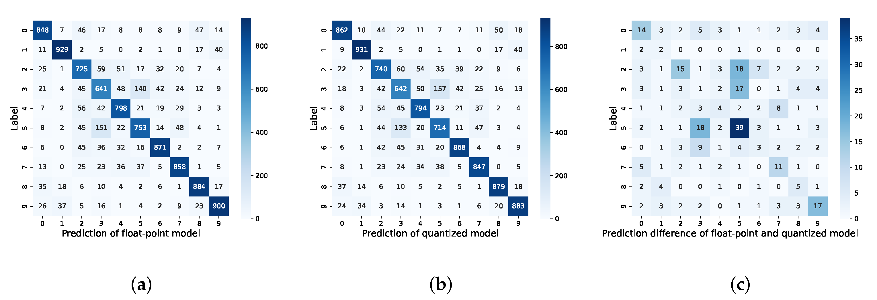
The quantized model shown in Figure 1b was trained using the conventional loss function $L_T$, which is the CE loss between the predictions of the quantized model and the labels. In contrast, we trained the quantized model using $L_F$, which is the MCL loss between the predictions of the quantized and floating-point models. The accuracy and CD values of the quantized model obtained using these two different methods on the 10-class labels of the CIFAR-10 dataset are shown in

Table 2. Accuracy (Acc.) and CD of the LeNet model, including the 32-bit floating-point model (FP32) and the 8-bit quantized model (ISE8). The quantized model is trained using different loss functions, in which $L_T$ is the CE loss between the predictions of the quantized model and the labels, and $L_F$ is the MCL loss between the predictions of the quantized and floating-point models.

Model	Acc. (%)											CD (%)
	Truck	Ship	Horse	Frog	Dog	Deer	Cat	Bird	Car	Plane	All
FP32	84.8	92.9	72.5	64.1	79.8	75.3	87.1	85.8	88.4	90.0	82.07	-
ISE8 ($L_T$)	86.2	93.1	74.0	64.2	79.4	71.4	86.8	84.7	87.9	88.3	81.60	4.06
ISE8 ($L_F$)	85.1	93.5	72.6	64.7	79.2	74.3	86.1	84.6	87.5	88.2	81.58	3.54

.

The quantized model trained using $L_F$ achieved an accuracy of 81.58%, which was 0.49% lower than that of the original model and only 0.02% lower than that of the quantized model trained using $L_T$. In addition, the quantized model trained using $L_F$ achieved a CD of 3.54%, which was 0.52% lower than that of the quantized model trained using $L_T$. This means that the quantized model trained using $L_F$ is more equivalent to the original model.

The decrease in accuracy resulted from increased prediction accuracy in four out of ten classes but decreased accuracy in the remaining six. As a result, these changes caused a decrease in the similarity between the quantized and floating-point models. Compared to the quantized model trained using $L_T$, the results varied when using $L_F$ to train the quantized model. Although quantization caused some loss, it reduced the CD by 0.49% while only decreasing the accuracy by 0.02%.

We show the confusion matrix of the outputs of the quantized model trained using the MCL and the floating-point model trained using $L_T$, which is presented in Figure 9. The outputs of the quantized model trained using the MCL show smaller differences when compared to the floating-point model, indicating a reduced equivalence loss. When comparing the prediction difference in Figure 9 with that in Figure 1, it can be seen that the maximum discrepancy in the classification predictions decreased from 39 (in Figure 1c) to 18 (in Figure 9c), and the number of instances where the prediction discrepancy exceeds 10 was reduced from 8 (in Figure 1c) to 5 (in Figure 9c). These results demonstrate the advantages of employing MCL training in quantized models to reduce the equivalence loss.

4.2. Evaluation on ImageNet

To demonstrate the effectiveness of the proposed method, we quantized several representative models using the MCL loss, including ResNet18/34/50, MobileNetV2, and BN-VGG16. Additionally, we evaluated them using 8-bit-width quantization on the ImageNet dataset.

We followed the proposed quantization scheme. First, we trained a 32-bit floating-point model using $L_T$ as the full-precision model. Then, we used it as an initial model to train the quantized model, where two of the loss functions were used: $L_T$ and $L_F$. Furthermore, we used identical training settings for pretraining and fine-tuning, including the learning rate, learning rate scheduler, batch size, optimizer, and weight decay.

For a better comparison, the initial learning rate in the training of the quantized model using $L_F$ remained unchanged in the training of the quantized model using $L_T$. The learning rate was updated every 20 epochs with the learning rate scheduler. The parameters were quantized by 10% every two epochs, and by the 20th epoch, all parameters were transferred to the ISE type. We used the stochastic gradient descent (SGD) optimizer to adjust the parameters. The momentum remained at 0.9, and the weight decay was set to $4\times {10}^{-5}$. For ResNet18/34 and MobileNetV2, the batch size was set to 128, and for ResNet50 and BN-VGG16, the batch size was set to 64 owing to their large size.

First, we compared the accuracy and CD of the quantized models obtained using different loss functions. The experimental results of these models on the ImageNet dataset are shown in

Table 3. Top-1 accuracy (Top-1 Acc.) of the 32-bit floating-point (FP32) model and 8/7-bit quantized (ISE8/7) model trained using different loss functions on the ImageNet dataset. $L_T$ is the CE loss between the predictions of the quantized model and the labels, and $L_F$ is the MCL loss between the predictions of the quantized and floating-point models. The CD is computed between the FP32 and the ISE8 model. The differences in the accuracy and CD values between both quantized models are indicated in bold type.

Model	Result	ResNet18	ResNet34	ResNet50	MobileNetV2	BN-VGG16
FP32	Top-1 Acc. (%)	70.63	74.72	76.87	71.97	74.31
ISE8 ($L_T$)	Top-1 Acc. (%)	70.13	73.90	76.16	69.12	72.61
	CD (%)	8.75	8.92	8.71	15.15	12.43
ISE8 ($L_F$)	Top-1 Acc. (%)	70.08 (−0.05)	74.11 (+0.21)	76.16 (+0.00)	69.33 (+0.21)	73.70 (+1.09)
	CD (%)	7.45 (−1.3)	7.48 (−1.44)	8.52 (−0.19)	13.32 (−1.83)	9.46 (−2.97)
ISE7 ($L_T$)	Top-1 Acc. (%)	69.18	73.32	75.43	61.23	71.10
	CD (%)	13.89	15.04	13.32	36.16	13.13
ISE7 ($L_F$)	Top-1 Acc. (%)	68.85 (−0.33)	73.71 (+0.39)	75.91 (+0.48)	61.48 (+0.25)	72.39 (+1.39)
	CD (%)	12.21 (−1.68)	12.90 (−2.14)	12.90 (−0.42)	27.40 (−8.76)	10.22 (−2.91)

, where we list the Top-1 accuracy (Top-1 Acc.) and CD of the quantized models.

We also present the accuracy of the floating-point model as a baseline. The two quantized models were trained using two different loss functions and identical quantization settings. We found that the quantized model trained using $L_F$ achieved the lowest CD while maintaining comparable or even higher performance compared to the quantized model trained using $L_T$. We can see that the network with the best performance is ResNet50 for 7-bit quantization, which achieved a CD of 12.90%, and the accuracy was higher than that of the quantized model trained using $L_T$ by 0.48%.

In addition, we compared the models quantized using many advanced methods, including FAQ [48], regularization [39], LSQ [40], EQ [41], QAT [30], OCS [42], ACIQ [43], SSBD [49], UNIQ [44], Apprentice [45], INQ [38], RV-Quant [46], 8-bit training [50], and ZeroQ [47]. The comparison was performed across different bit widths of the weights and activations. For most of these methods, bias quantization is not mentioned, whereas our method can support bias quantization at a low bit width. For all methods, the Top-1 accuracy (Top-1 Acc.) serves as the baseline for the floating-point model. The experimental results on the ImageNet dataset for these models are shown in

Table 4. Top-1 accuracy (Top-1 Acc.) results on the ImageNet dataset for ResNet18 are displayed as weights (W), activations (A), and biases (B). Our proposed method uses $L_F$ as a loss function to train quantized models. The CD results are shown in brackets to the right of the accuracy results. The comparison results for fair comparison and reference comparison are presented in the table. The best results are marked in red, and our results are indicated in bold type.

ResNet18
Comparison	Method	Bit	Top-1 Acc. (%)
Fair	FAQ	W8A8B32	70.02
	Regularization	W8A8	68.10
	INQ	W8A8	68.96
	RV-Quant	W8A8	70.01
	8-bit training	W8A8	66.95
	Ours	W8A8B8	70.08 (7.48)
Reference	FAQ	W4A4B32	69.82
	Regularization	W4A4	67.50
	UNIQ	W4A8	67.02
	UNIQ	W5A8	68.00
	ACIQ	W8A4	65.80
	Ours	W7A7B7	68.85 (12.21)
-	Baseline	W32A32B32	70.63

,

Table 5. Top-1 accuracy on the ImageNet dataset for ResNet34. The table description is consistent with Table 4.

ResNet34
Comparison	Method	Bit	Top-1 Acc. (%)
Reference	LSQ	W8A8	74.10
	FAQ	W8A8B32	73.71
	Ours	W8A8B8	74.11 (7.48)
Reference	Apprentice	W4A8	73.10
	UNIQ	W4A8	71.09
	UNIQ	W5A8	72.60
	FAQ	W4A4B32	73.31
	Ours	W7A7B7	73.71 (12.90)
-	Baseline	W32A32B32	74.72

,

Table 6. Top-1 accuracy on the ImageNet dataset for ResNet50. The table description is consistent with Table 4.

ResNet50
Comparison	Method	Bit	Top-1 Acc. (%)
Fair	EQ	W8A8	75.13
	RV-Quant	W8A8	75.67
	OCS	W8A8	75.70
	QAT	W8A8	75.10
	8-bit training	W8A8	71.72
	SSBD	W8A8B16	74.95
	Ours	W8A8B8	76.16 (8.52)
Fair	EQ	W7A7	75.04
	RV-Quant	W7A7	75.89
	Ours	W7A7B7	75.91 (12.90)
Reference	UNIQ	W4A8	73.37
	Apprentice	W4A8	74.70
	ACIQ	W8A4	71.45
	OCS	W6A8	75.20
	OCS	W7A8	75.50
	OCS	W8A6	63.60
	OCS	W8A7	74.50
-	Baseline	W32A32B32	76.87

,

Table 7. Top-1 accuracy on the ImageNet dataset for MobileNetV2. The table description is consistent with Table 4.

MobileNetV2
Comparison	Method	Bit	Top-1 Acc. (%)
Fair	RV-Quant	W8A8	70.29
	QAT	W8A8	70.90
	ZeroQ	W8A8	72.91
	Ours	W8A8B8	69.33 (13.32)
Reference	Ours	W7A7B7	61.48 (27.40)
-	Baseline	W32A32B32	71.97

and

Table 8. Top-1 accuracy on the ImageNet dataset for BN-VGG16. The table description is consistent with Table 4.

BN-VGG16
Comparison	Method	Bit	Top-1 Acc. (%)
Fair	FAQ	W8A8B32	73.66
	LSQ	W8A8	73.50
	EQ	W8A8	70.97
	OCS	W8A8	72.80
	Ours	W8A8B8	73.70 (9.46)
Fair	EQ	W7A7	70.96
	Ours	W7A7B7	72.39 (10.22)
Reference	FAQ	W4A8B32	73.66
	ACIQ	W8A4	67.60
	OCS	W6A8	72.10
	OCS	W7A8	72.60
	OCS	W8A6	49.20
	OCS	W8A7	70.70
-	Baseline	W32A32B32	74.31

. To the best of our knowledge, model quantization using the MCL loss exhibited the best performance, particularly for ResNet18/34/50 networks.

However, the results for MobileNetV2 were significantly lower compared to those of the other models. The CD did not fall below 10% for the 8-bit setting and was close to 30% for the 7-bit setting. We presume that the reason for this is that MobileNetV2, as a lightweight model, contains inverted residuals and depth-wise convolution layers. These structures have far fewer parameters compared to conventional convolutional layers with kernel sizes of 3, 5, 7, etc. To a certain extent, this increased the impact of parameter quantization on the results. To further investigate the reasons, we generated a kernel density estimation (KDE) of the parameter distributions for the floating-point and quantized models in MobileNetV2. For comparative purposes, we also included KDE for BN-VGG16, as illustrated in Figure 10.

For the MobileNetV2 and BN-VGG16 networks, we generated the weight distribution of the continuous convolution/linear layer and batch normalization layer of the network, which are located at the front and back layers of the model, respectively, as shown in Figure 10. Owing to insufficient data, the impact of the bias was negligible. Conv/Linear-0/1 and BN-0/1 are two consecutive computing layers. It should be noted here that the weight of the batch normalization layer refers to the weight after fusing the variance of the input feature map. The black line represents the weight distribution of the floating-point model, whereas the blue and orange lines represent that of the quantized model trained using $L_T$ and $L_F$, respectively. For the parameter distributions of the convolutional or linear layers, we observe an almost complete overlap, demonstrating an approximate normal distribution for both models. This is in line with the original purpose of quantization, which aims for the quantized weights to resemble floating-point weights as much as possible. However, the situation is slightly different for the parameter distribution in the batch normalization layer. On the one hand, there are generally fewer parameters in the batch normalization layer compared to the convolutional/linear layers, resulting in a greater difference in the data distribution. As shown in Figure 10, the weight distribution of the 8-bit quantized model trained using $L_T$ and $L_F$ was challenging to approximate or match that of the 32-bit floating-point model. On the other hand, the fused weight of the batch normalization layer includes variance information from the feature map, which means that inadequate or incomplete feature extraction can significantly affect the overall data distribution.

For BN-VGG16, the convolution layer with a kernel size of three contained many weight parameters (Param = 1792 and 1,180,160), which extracted feature information well. As a result, the subsequent batch normalization layer approximated a normal distribution. Moreover, compared to the quantized model trained using $L_T$, the weight distribution of the quantized BN-VGG16 trained using $L_F$ approached the floating-point BN-VGG16 model more closely. As shown in Figure 10, the orange line is closer to the black line than the blue line.

In contrast, for MobileNetV2, the number of weight parameters was significantly smaller compared to BN-VGG16 (Param = 528 and 442,752). Insufficient feature information led to a feature distribution with a large variance, which further affected the distribution of the fused weight in the subsequent batch normalization layer. This impact became increasingly pronounced as the layer moved further back. As shown in Figure 10, the weight distribution of BN-0 roughly resembles a normal distribution, whereas that of the BN-1 layer at the back deviates completely from a normal distribution.

Consequently, the 8-bit quantized model output differed significantly from that of the floating-point model for MobileNetV2. The quantized model trained using $L_F$ achieved a significant reduction in the CD of up to 13.32% while experiencing a notable increase in accuracy of 69.33%, which was higher than that of the quantized model trained using $L_T$.

In summary, the results prove that in most cases, the quantized model trained using $L_F$ can further reduce the mode compression loss while maintaining or even improving the accuracy.

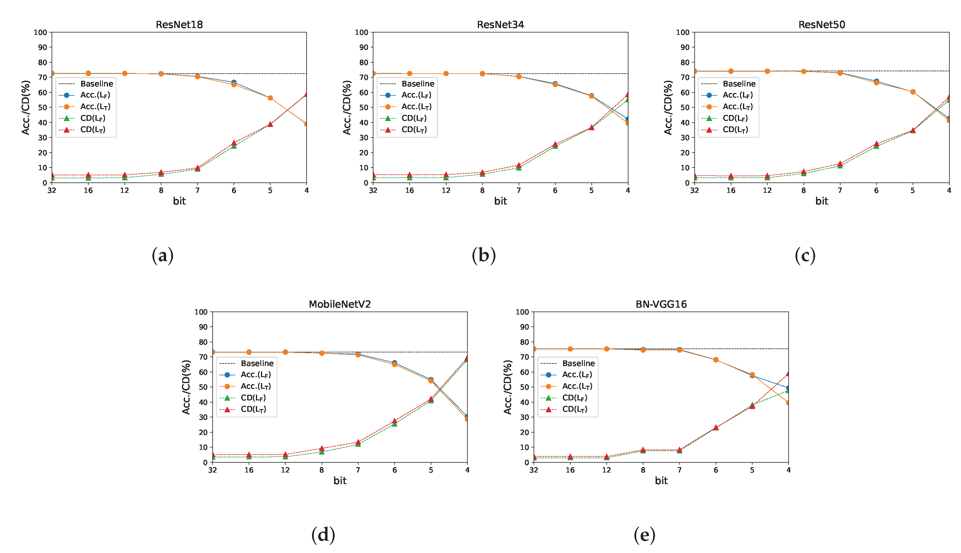
4.3. Evaluation on CIFAR-100

To evaluate the CD of the quantization model at various bit widths, we trained the ResNet18/34/50 network on the CIFAR-100 dataset at bit widths of 32, 16, 12, 8, 7, and 6. The loss functions we used were $L_F$ and $L_T$. The Top-1 accuracy (Top-1 Acc.) and CD changes in the different network models at different quantization bit widths are illustrated in Figure 11.

The use of different loss functions resulted in few differences in the networks’ accuracy values for the quantization models at different bit widths. This is evidenced by the similar orange and blue lines in the graph, with differences becoming more prominent only when the quantization bit width decreased. However, for the CD, training using the MCL loss function yielded a smaller compression loss, as indicated by the green line, which is lower than the red line in the graph. In addition, the CD increased with decreasing bit widths of quantization. Similarly, at lower bit widths, the difference in the CD became more pronounced. The quantized model trained using $L_F$ achieved higher accuracy compared to the one trained using $L_T$ when the bit width was lower than six. This was particularly evident for BN-VGG16 and ResNet34 with a 4-bit width. The quantization models with different bit widths not only resulted in different levels of performance but also lower bandwidths, thereby reducing the demand for storage and making deployment on resource-constrained devices more feasible. The CD of the quantization model fine-tuned using the MCL was lower, making it better suited to scenarios that require high equivalence between the quantization and floating-point models (such as intelligent face locks, etc.).

5. Conclusions

We proposed a novel quantization pipeline named DiffQuant, which includes the compression difference (CD) and model compression loss (MCL). The CD measures the equivalence of quantized and floating-point models, and the MCL leverages the output from both models to guide fine-tuning.

Furthermore, we developed a quantization algorithm named DiffQuant, which utilizes the ISE as the data type and the MCL as a loss function, to fine-tune the quantized model. This proposed method can quantize both the batch normalization (BN) layer and the bias when supporting the quantization of weights and activations using unlabeled datasets.

Various experiments on the CIFAR-100 and ImageNet datasets demonstrated that the quantized model trained using the MCL achieved a significantly lower compression loss compared to traditional methods while maintaining accuracy. For lightweight models such as MobileNetV2, we compared and analyzed the weight distribution of the quantized model. The results showed that the feature extraction process had a critical impact on the weight distribution, particularly for batch normalization, leading to an inevitable loss of model compression. Finally, we evaluated the performance of the quantized model at different bit widths. We found that the accuracy and CD decreased with a reduction in the bit width. The quantized model trained using the MCL consistently showed low compression loss and high accuracy. Furthermore, the MCL calculates the loss between the outputs of the quantized and floating-point models. However, this measurement may be susceptible to outliers. In future work, we plan to address this issue by utilizing more stable loss functions for evaluation. We also intend to explore the impact of the MCL on the performance of the quantized model by combining a conventional loss function (such as the cross-entropy loss between the quantized model’s output and labels, etc.) with the MCL in different proportions.

References

1. Wang, Y.; Wang, C.; Long, P.; Gu, Y.; Li, W. Recent advances in 3D object detection based on RGB-D: A survey. Displays 2021, 70, 102077. [Google Scholar] [CrossRef]
2. Ning, E.; Wang, C.; Zhang, H.; Ning, X.; Tiwari, P. Occluded person re-identification with deep learning: A survey and perspectives. Expert Syst. Appl. 2023, 239, 122419. [Google Scholar] [CrossRef]
3. He, K.; Zhang, X.; Ren, S.; Sun, J. Deep residual learning for image recognition. In Proceedings of the Conference on Computer Vision and Pattern Recognition, Las Vegas, NV, USA, 27–30 June 2016; pp. 770–778. [Google Scholar]
4. Li, S.; Dong, X.; Shi, Y.; Lu, B.; Sun, L.; Li, W. Multi-angle head pose classification with masks based on color texture analysis and stack generalization. Concurr. Comput. Pract. Exp. 2023, 35, e6331. [Google Scholar] [CrossRef] [PubMed]
5. Tian, S.; Li, L.; Li, W.; Ran, H.; Ning, X.; Tiwari, P. A survey on few-shot class-incremental learning. Neural Netw. 2024, 169, 307–324. [Google Scholar] [CrossRef] [PubMed]
6. Long, J.; Shelhamer, E.; Darrell, T. Fully convolutional networks for semantic segmentation. In Proceedings of the IEEE Conference on Computer Vision and Pattern Recognition, Boston, MA, USA, 7–12 June 2015; pp. 3431–3440. [Google Scholar]
7. Hinton, G.; Vinyals, O.; Dean, J. Distilling the Knowledge in a Neural Network. arXiv 2015, arXiv:1503.02531. [Google Scholar]
8. Han, S.; Pool, J.; Dally, W.J. Learning both Weights and Connections for Efficient Neural Networks. In Proceedings of the Advances in Neural Information Processing Systems, Montreal, QC, Canada, 7–12 December 2015; Volume 28. [Google Scholar]
9. Jacob, B.; Kligys, S.; Chen, B.; Zhu, M.; Tang, M.; Howard, A.; Adam, H. Quantization and training of neural networks for efficient integer-arithmetic-only inference. In Proceedings of the IEEE Conference on Computer Vision and Pattern Recognition, Salt Lake City, UT, USA, 18–23 June 2018; pp. 2704–2713. [Google Scholar]
10. Courbariaux, M.; Bengio, Y.; David, J.P. Training deep neural networks with low precision multiplications. arXiv 2014, arXiv:1412.7024. [Google Scholar]
11. Zhou, S.; Wu, Y.; Ni, Z.; Zhou, X.; Wen, H.; Zou, Y. Dorefa-net: Training low bitwidth convolutional neural networks with low bitwidth gradients. In Proceedings of the IEEE Conference on Computer Vision and Pattern Recognition, Honolulu, HI, USA, 21–26 July 2017; pp. 442–450. [Google Scholar]
12. Cheng, Q.; Yang, Y.; Guo, Y. Review on Neural Network Compression. Appl. Sci. 2020, 10, 3978. [Google Scholar]
13. Khoramshahi, E.; Liu, Z.; McDonald-Maier, K.D. Rethinking the Structure of Redundant Convolutional Neural Networks for Efficient Inference. IEEE Access 2020, 8, 16837–16850. [Google Scholar]
14. Leng, C.; Dou, Z.; Li, H.; Zhu, S.; Jin, R. Extremely low bit neural network: Squeeze the last bit out with admm. In Proceedings of the Thirty-Second AAAI Conference on Artificial Intelligence, New Orleans, LA, USA, 2–7 February 2018. [Google Scholar]
15. Mishra, A.; Nurvitadhi, E.; Cook, J.J.; Marr, D. Wrpn: Wide reduced-precision networks. arXiv 2017, arXiv:1709.01134. [Google Scholar]
16. Xu, C.; Yao, J.; Lin, Z.; Ou, W.; Cao, Y.; Wang, Z.; Zha, H. Alternating multi-bit quantization for recurrent neural networks. arXiv 2018, arXiv:1802.00150. [Google Scholar]
17. Zhou, S.C.; Wang, Y.Z.; Wen, H.; He, Q.Y.; Zou, Y.H. Balanced quantization: An effective and efficient approach to quantized neural networks. J. Comput. Sci. Technol. 2017, 32, 667–682. [Google Scholar] [CrossRef]
18. Zhou, W.; Wang, A.; Yu, L. A Heart Sound Diagnosis Processing Unit Based on LSTM Neural Network. In Proceedings of the 2022 IEEE 4th International Conference on Circuits and Systems (ICCS), Chengdu, China, 23–26 September 2022; pp. 210–215. [Google Scholar]
19. Cai, H.; Zhu, L.; Han, S. Proxylessnas: Direct neural architecture search on target task and hardware. arXiv 2018, arXiv:1812.00332. [Google Scholar]
20. Li, Y.; Jin, X.; Mei, J.; Lian, X.; Yang, L.; Xie, C.; Yu, Q.; Zhou, Y.; Bai, S.; Yuille, A. Autonl: Neural architecture search for lightweight non-local networks in mobile vision. In Proceedings of the International Conference on Learning Representations, Addis Ababa, Ethiopia, 26–30 April 2020. [Google Scholar]
21. Liu, C.; Zoph, B.; Neumann, M.; Shlens, J.; Hua, W.; Li, L.J.; Fei-Fei, L.; Yuille, A.; Huang, J.; Murphy, K. Progressive neural architecture search. In Proceedings of the European Conference on Computer Vision (ECCV), Munich, Germany, 8–14 September 2018; pp. 19–34. [Google Scholar]
22. Mei, J.; Li, Y.; Lian, X.; Jin, X.; Yang, L.; Yuille, A.; Yang, J. Atomnas: Fine-grained end-to-end neural architecture search. In Proceedings of the International Conference on Learning Representations, Addis Ababa, Ethiopia, 26–30 April 2020. [Google Scholar]
23. Pham, H.; Guan, M.Y.; Zoph, B.; Le, Q.V.; Dean, J. Efficient neural architecture search via parameter sharing. arXiv 2018, arXiv:1802.03268. [Google Scholar]
24. Wu, B.; Dai, X.; Zhang, P.; Wang, Y.; Sun, F.; Wu, Y.; Tian, Y.; Vajda, P.; Jia, Y.; Keutzer, K. Fbnet: Hardware-aware efficient convnet design via differentiable neural architecture search. In Proceedings of the IEEE Conference on Computer Vision and Pattern Recognition, Long Beach, CA, USA, 15–19 June 2019; pp. 10734–10742. [Google Scholar]
25. Xie, S.; Zheng, H.; Liu, C.; Lin, L. Snas: Stochastic neural architecture search. arXiv 2018, arXiv:1812.09926. [Google Scholar]
26. Elthakeb, A.T.; Pilligundla, P.; Mireshghallah, F.; Yazdanbakhsh, A.; Gao, S.; Esmaeilzadeh, H. Releq: An automatic reinforcement learning approach for deep quantization of neural networks. arXiv 2018, arXiv:1811.01704. [Google Scholar] [CrossRef] [PubMed]
27. Wu, B.; Wang, Y.; Zhang, P.; Tian, Y.; Vajda, P.; Keutzer, K. Mixed precision quantization of convnets via differentiable neural architecture search. arXiv 2018, arXiv:1812.00090. [Google Scholar]
28. Uhlich, S.; Mauch, L.; Yoshiyama, K.; Cardinaux, F.; Garcia, J.A.; Tiedemann, S.; Kemp, T.; Nakamura, A. Differentiable quantization of deep neural networks. arXiv 2019, arXiv:1905.11452. [Google Scholar]
29. Wang, K.; Liu, Z.; Lin, Y.; Lin, J.; Han, S. Haq: Hardware-aware automated quantization with mixed precision. In Proceedings of the IEEE Conference on Computer Vision and Pattern Recognition, Long Beach, CA, USA, 15–19 June 2019; pp. 8612–8620. [Google Scholar]
30. Krishnamoorthi, R. Quantizing deep convolutional networks for efficient inference: A whitepaper. arXiv 2018, arXiv:1806.08342. [Google Scholar]
31. Zhang, Y.; Ye, J.; Zhang, Y.; Qi, H. Data-Free Quantization with Accurate Activation Clipping and Adaptive Batch Normalization. Neural Process. Lett. 2023, 55, 10555–10568. [Google Scholar]
32. Cai, H.; Chen, Y.; Zhang, W.; Xiong, J.; Lin, S. Generative Low-Bitwidth Data Free Quantization. arXiv 2020, arXiv:2003.03603. [Google Scholar]
33. Choi, T.; Park, J.; Shin, S.J. Data-Free Network Quantization with Adversarial Knowledge Distillation. In Proceedings of the IEEE/CVF Conference on Computer Vision and Pattern Recognition (CVPR) Workshops, Seattle, WA, USA, 13–19 June 2020. [Google Scholar]
34. He, Y.; Kang, G. Data-Free Quantization through Weight Equalization and Bias Correction. arXiv 2019, arXiv:1906.04721. [Google Scholar]
35. Yang, H.; Xu, J.; Yang, G.; Zhang, M.; Qin, H. Neural Network Quantization Based on Model Equivalence. In Proceedings of the 2022 International Conference on High Performance Big Data and Intelligent Systems (HDIS), Tianjin, China, 10–11 December 2022; pp. 8–12. [Google Scholar]
36. Lin, D.D.; Talathi, S.S.; Annapureddy, V.S. Fixed Point Quantization of Deep Convolutional Networks. In Proceedings of the 33rd International Conference on Machine Learning, New York, NY, USA, 19–24 June 2016. [Google Scholar]
37. Rastegari, M.; Ordonez, V.; Redmon, J.; Farhadi, A. XNOR-Net: ImageNet Classification Using Binary Convolutional Neural Networks. arXiv 2016, arXiv:1603.05279. [Google Scholar]
38. Zhou, A.; Yao, A.; Guo, Y.; Xu, L.; Chen, Y. Incremental network quantization: Towards lossless cnns with low-precision weights. In Proceedings of the IEEE Conference on Computer Vision and Pattern Recognition, Honolulu, HI, USA, 21–26 July 2017; pp. 3306–3314. [Google Scholar]
39. Liu, S.; Liu, M.; Zhao, R.; Yang, D.; Cheng, X.; Chen, Y. Learning Sparse Low-Precision Neural Networks with Learnable Regularization. In Proceedings of the 27th ACM International Conference on Multimedia, Nice, France, 21–25 October 2019; pp. 2163–2166. [Google Scholar]
40. Zhang, S.; Zhou, Z.; Lin, J.; Sun, J. Learned step size quantization. In Proceedings of the IEEE Conference on Computer Vision and Pattern Recognition, Salt Lake City, UT, USA, 18–23 June 2018; pp. 4641–4650. [Google Scholar]
41. Wang, Y.; Liu, J.; Su, H.; Yang, Y.; Li, W. EasyQuant: Post-training quantization via scale optimization. arXiv 2021, arXiv:2006.16669. [Google Scholar]
42. Zhu, C.; Han, S. Improving neural network quantization without retraining using outlier channel splitting. arXiv 2017, arXiv:1711.01577. [Google Scholar]
43. Banner, R.; Nahshan, Y.; Hoffer, E.; Soudry, D. ACIQ: Analytical clipping for integer quantization of neural networks. arXiv 2018, arXiv:1810.05723v1. [Google Scholar]
44. Li, B.; Wang, X.; Zhang, L.; Liu, H.; Liu, Y.; Cheng, J. UNIQ: Uniform noise injection for the quantization of neural networks. In Proceedings of the IEEE Conference on Computer Vision and Pattern Recognition, Long Beach, CA, USA, 15–20 June 2019; pp. 5714–5722. [Google Scholar]
45. Mishra, A.; Marr, D. Apprentice: Using knowledge distillation techniques to improve low-precision network accuracy. In Proceedings of the IEEE Conference on Computer Vision and Pattern Recognition Workshops, Salt Lake City, UT, USA, 18–22 June 2018; pp. 18–25. [Google Scholar]
46. Belaouad, M.; Moerman, B.; Verbelen, T.; Dambre, J. Value-aware Quantization for Training and Inference of Neural Networks. In Proceedings of the European Conference on Computer Vision (ECCV), Munich, Germany, 8–14 September 2018. [Google Scholar]
47. Wang, T.; Liu, Z.; Chen, Z.; Xu, C.; Wu, X. ZeroQ: A Novel Zero Shot Quantization Framework. In Proceedings of the AAAI Conference on Artificial Intelligence, New York, NY, USA, 7–12 February 2020; Volume 34, pp. 11654–11661. [Google Scholar]
48. Zhu, H.; Zhong, Z.; Deng, Y.; Liu, J.; Wu, J.; Xiong, H. Discovering low-precision networks close to full-precision networks for efficient embedded inference. In Proceedings of the International Conference on Learning Representations, Addis Ababa, Ethiopia, 26–30 April 2020. [Google Scholar]
49. Blalock, D.; Yang, C.H.; Shankar, V.; Krishnamurthy, A.; Zhang, Y.; Hsia, J.; Keutzer, K. Same, same but different: Recovering neural network quantization error through weight factorization. In Proceedings of the International Conference on Learning Representations, Addis Ababa, Ethiopia, 26–30 April 2020. [Google Scholar]
50. Gupta, S.; Agrawal, A.; Gopalakrishnan, K.; Narayanan, P. Training deep neural networks with 8-bit floating point numbers. In Proceedings of the International Conference on Machine Learning, Lille, France, 6–11 July 2015; pp. 1737–1746. [Google Scholar]
Figure 1. Confusion matrices showing (a) the labels and predictions of the floating-point model, (b) the labels and predictions of the quantized model, and (c) the labels and prediction differences between the floating-point and quantized models. Darker blue means more samples.
Electronics 12 04972 g001
Figure 2. Mapping from real numbers to integer values: (a) affine quantization, (b) scale quantization. The solid black line represents the mapping of values, and the dotted red line represents the boundary of the mapping. The gray areas indicate the truncated values.
Electronics 12 04972 g002
Figure 3. Calculation of loss functions, in which L T is the loss function between the output of the quantized model and the labels, and L F is the loss function between the outputs of the quantized and floating-point models. FP32 represents the 32-bit floating-point type and ISE indicates the integer type with shared exponent.
Electronics 12 04972 g003
Figure 4. Achieving the optimal shared exponent by measuring the distance between the real and quantized data and computing the PCC and JSD. r indicates real data with the floating-point type. Quantized data are represented with a pseudo-floating-point type.
Electronics 12 04972 g004
Figure 5. Probability density histogram of floating-point data and probability density distribution of pseudo-floating-point data across different reference shared exponents.
Electronics 12 04972 g005
Figure 6. A flowchart of the quantization process.
Electronics 12 04972 g006
Figure 7. Training and inference pipelines of DiffQuant using ISE. Parameters in the batch normalization layer are updated during the training phase and then fused during the inference phase.
Electronics 12 04972 g007
Figure 8. Simulation of hardware computing process using RNT and OTP. N is the bit width and L is the bit width of the intermediate results, widened so as not to lose accuracy.
Electronics 12 04972 g008
Figure 9. Confusion matrices showing (a) the labels and predictions of the floating-point model, (b) the labels and predictions of the quantized model trained using the MCL, and (c) the labels and prediction differences between the floating-point and quantized models. Darker blue means more samples.
Electronics 12 04972 g009
Figure 10. Weight KDE for MobileNetV2 and BN-VGG16 in convolution (a,b,e,f) and batch normalization layers (c,d,g,h), respectively. In the title of each subfigure, “0” and “1” indicate the two successive layers, where the former refers to the layer near the front of the network, and the latter represents that near the back. Param represents the number of parameters. The comparison model includes the FP32 and the ISE8 models trained using different loss functions, in which L T is the CE loss between the predictions of the quantized model and the labels, and L F is the MSE loss between the predictions of the quantized and floating-point models.
Electronics 12 04972 g010aElectronics 12 04972 g010b
Figure 11. The accuracy (Acc.) and CD variations using different quantization bit widths on the CIFAR-10 dataset. The results for ResNet18, ResNet34, ResNet50, MobileNetV2, and BN-VGG16 are illustrated in subfigures (a), (b), (c), (d), and (e), respectively. The baseline indicates the accuracy of the FP32 model.
Electronics 12 04972 g011