Urban Traffic Simulation Using Mobility Patterns Synthesized from Real Sensors

Abstract

Smart cities are an ongoing research topic with multiple sub-research areas, from traffic control to optimization and even safety. However, testing the new methodologies or technologies directly in the real world is an almost impossible feat that, inclusively, can result in disaster. Thus, there is the importance of simulation. Simulation enables testing new and complex methodologies and gauging their impact in a realistic context without adding any safety issues. Additionally, these can accurately map real-world conditions depending on the simulation configuration. One key aspect of the simulation is the traffic flows in the simulated region. These may be hard to find and, if ill-set, may introduce bias in the results. This work is on the characterization of the traffic in the city center of Guimarães, Portugal. An urban simulation scenario was established, using SUMO as the mobility traffic simulator, with traffic patterns derived from real-world data provided by Guimarães City Hall and using Eclipse MOSAIC for extended vehicular simulation. Apart from mobility patterns analysis, this work also provides publicly accessible datasets, simulations, and applications made available to future research works.

1. Introduction

The increase in vehicle and pedestrian traffic in cities can sometimes overwhelm traditional traffic management. Current research on smart cities aims to improve many aspects of this, inclusively optimizing traffic flows.

This research type needs accurate data to replicate real city contexts. Otherwise, bias can be easily introduced, as traffic can be very complex.

This work analyzes real traffic data provided by the Guimarães City Hall, collected from multiple monitoring points in the city. These data may be used to describe the traffic and replicate it in simulation. The goal is to produce realistic datasets and a ready simulation to be used in future research works.

Guimarães (https://www.cm-guimaraes.pt/, accessed on 1 November 2023) is a city in the northern part of Portugal, known for being the birthplace of the country, and it is currently part of Unesco’s World Heritage. According to the latest statistics from Instituto Nacional de Estatıistica (INE), it has 156 thousand inhabitants.

Simulations are built using Simulation of Urban MObility (SUMO) [1], one of the most used traffic simulators, coupled with Eclipse Multi-Domain and Multi-Scale Simulation framework for Connected and Automated Mobility (MOSAIC). Coupling these simulators enables more complete and complex scenarios, including the implementation of Intelligent Transportation System (ITS) applications on vehicles, traffic lights, or Road Side Unit (RSUs). It also enables all the road entities to communicate, opening the possibility for new use cases. Thus, using MOSAIC to create the simulation can provide a set of valuable tools for future work. Among its capabilities, MOSAIC empowers real-time adjustments, such as dynamic vehicle re-routing and adaptive traffic light changes, in response to simulation events. Consequently, building a MOSAIC-based simulation aims to provide instruments for future developments, enabling the development of more intricate and sophisticated applications. This approach proves especially beneficial in assessing behavioral dynamics within smart cities, contributing to their overall evolution.

The main outcome of this work is the replication of real-world traffic using a simulation framework instead of the more traditional approach of using a traffic simulator. This approach enables a plethora of new functionalities and use cases that can further expand the research. Moreover, the simulation scenario created and its traffic flows were analyzed to gauge the implications of traffic phenomena, such as stopped time, on the fuel consumption and emissions produced.

Results showed that the SUMO simulator could replicate the real scenario accurately. Additionally, this work produced a set of datasets containing multiple movement parameters from the vehicles, including fuel consumption, CO2, CO, HC, PMx, NOx emissions, and vehicles stopped time. This dataset is available to download at https://doi.org/10.5281/zenodo.7997433 (accessed on 1 November 2023), and the code used to produce these results at https://github.com/fabio-r-goncalves/norte (accessed on 1 November 2023).

This paper is organized as follows. Section 2 presents a review of the related work surrounding the use of simulation to mimic traffic behavior and the different types of data that can feed these simulations. Section 3 presents the simulator and the simulation frameworks used to increase its realism. In Section 4 and Section 5, the city center that will be simulated is presented, as well as the way the traffic data—including vehicle, bus, and traffic light data—were gathered and prepared. Section 6 presents the process of modeling the data available to replicate the real-world traffic in the simulator. Results are presented and discussed in Section 7. The paper concludes with remarks about the work developed and some pointers towards future work.

2. Related Work

Simulation is the representation of a real situation or system in software, replicating its behaviors, interactions, and environmental characteristics. A simulation model allows for the understanding of the current state of a system and the evaluation of the effects that different scenarios can have on it. Then, when a system is studied through the use of simulation, theoretical changes can be tested and validated. The legitimacy of the simulation result is directly related to the quality of the information used and its integration into the simulation system [2]. Simulation models are a tool to analyze dynamic systems and offer a risk-free alternative to test different configurations without having to implement them in the real world and thus avoiding unnecessary costs [3].

Simulation models can be of three different types: macroscopic, mesoscopic, and microscopic models. Macroscopic models represent the system in a highly abstract form where each object and all the interactions between them are not computed. The objects in the simulation are grouped in clusters, and only their quantity and flow are taken into account. In this way, this type of model offers fast execution times; however, the results produced are less accurate. On the other side of the spectrum when compared with macroscopic models, microscopic models represent the system as detailed as in reality. Abstraction is kept at a minimum, and all behaviors, dimensions, distances, speeds, and interactions are needed and implemented into the model. The results obtained are extremely detailed, allowing for a complete study of the system, but its processing can be lengthy on highly complex or large systems [4,5]. A middle-ground solution are the mesoscopic models. This type of model balances the compromise between the accuracy of the results and the running times [6], and achieves better results and lower processing times than the macroscopic and microscopic models, respectively.

Transitioning simulation to the study of traffic, microscopic simulation models, because of their characteristics, are the ones that better reproduce the behavior of vehicles. Among the available traffic simulators and considering the project’s needs, SUMO edges out the others by being free and open-source [7].

In the literature, there are various strategies to model the real world in the SUMO simulator. In 2013, Ref. [8] used the SUMO simulator to model the city of Coimbra, Portugal. Traffic routes were modeled based on an origin–destination matrix built from mobility information collected through GPS, road sensors, and historical data. The network was imported from the world map platform Open Street Map (OSM). The results showed that SUMO was able to represent the urban traffic realistically, concluding that SUMO was a good choice for future works regarding road network management.

In Italy, Ref. [9] built a real-world traffic micro-simulation scenario from scratch with SUMO of the city of Cagliari. The aim of the work was to create a detailed step-by-step tutorial on how to use the different tools available on the SUMO package to build and run the simulation. Similarly to the previous paper, the transportation network was imported from OSM, and an origin–destination matrix with real traffic data was used for route generation. The author adds that the simulation model can be further developed to better aid decision-makers by adding multiple vehicle types, traffic lights, and public transport systems (buses).

Researchers from Croatia [10] used SUMO to build a simulation model of the city of Rijeka. The network was downloaded from OSM, and real data were collected for traffic generation. In this case, mobile data from a mobile phone network infrastructure provider was used to compute origin–destination matrices. The city map was divided into 48 zones, each with an origin and a destination. The total number of trips in the network resulted from the sum of the trips of each origin–destination combination. One adversity pointed out by the researchers was the number of routes that could be generated because those were limited by the data provider.

One increasingly explored area of research centers around traffic optimization. In the works referenced by [11,12,13], the Particle Swarm Optimization (PSO) algorithm is employed to enhance traffic flow within specific road segments or entire urban areas. Addressing traffic optimization encompasses various strategies, with one particularly subtle approach involving adjustments to traffic light timings.

In [14], Chi Liu et al. propose a new LSTM model, called “AttConvL-STM”, to predict the in/out flows within a short period of time within region in a city and they have analyzed the prediction results with baselines from three large public datasets in Beijing, Rome, and Chengdu. The authors also consider that their approach, which is able to perform multi-step-ahead predictions, is suitable to help city managers to identify crowd movements. The present work also aims similar objectives, but this time based upon the simulation of real traffic flows.

There are also works using SUMO and virtual traffic light systems [15] for urban traffic management, where vehicle mobility patterns and velocities are adjusted according to neighboring intersection contexts. Works presented in [16], using SUMO and Vehicles in Network Simulation (VEINS) [17] simulation tools, also show that urban traffic conditioning is also important to facilitate emergency vehicle movement by lowering emergency travel times.

While a considerable portion of the existing literature relies on replicating traffic patterns using tools like SUMO, a notable research gap emerges in the absence of bi-directional communication capabilities. This limitation, though valuable for certain applications, may hinder the potential for broader and more dynamic simulations in future studies. The present study elevates this research paradigm by introducing bi-directional communication (established between SUMO and the network simulator), thereby introducing many novel functionalities. Significant enhancements include the integration of intelligent traffic lights [15,18] and the utilization of communication-based strategies for the implementation of smart cities [19,20]. Moreover, the accurate replication of real-world traffic is of major importance to gauge the real improvement of the traffic caused by the algorithm.

3. Simulation Frameworks

Traffic simulations have a multitude of algorithms that can replicate real-world behavior quite well. There are multiple traffic simulators, including SUMO [1], AnyLogic [21], Vissim [22], and Aimsun [23]. SUMO is distributed as an open-source program, providing more flexibility than the others, and, as such, was the traffic simulator chosen for this work. It is a multi-modal traffic simulator, which makes it ideal for studying the movement of multiple modes of transportation. Being a microscopic simulator means that it enables controlling each vehicle and its parameters individually. SUMO provides tools to control multiple vehicle and movement parameters, including the speed, acceleration, following mode, and vehicle size.

Even though SUMO is quite powerful, it has its limitations. For example, it does not allow adjusting parameters during its run time. Moreover, vehicles, traffic lights, and other entities have static behavior. The presented drawbacks can be addressed using a simulation framework.

Simulation frameworks, such as VEINS [17], Eclipse Mosaic [24,25], and OMNET++ [26], can provide bi-directional communication between the traffic simulator and a network simulator, allowing it to extend its functionalities, allowing vehicle communications and the implementation of applications in the vehicles, thus giving the road entities some “intelligence”.

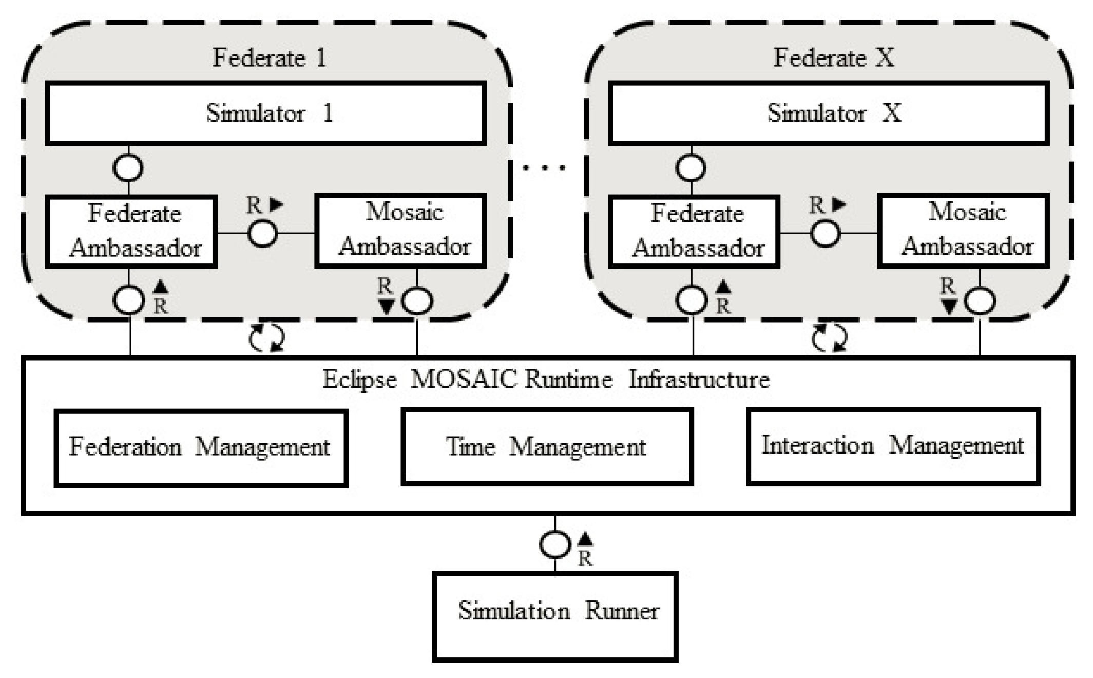
The simulation framework chosen for this work was Eclipse MOSAIC, Version 22.1. This is a Java-based open-source software distributed under the Eclipse Public License developed by DCAITI in Berlin, Germany. It is able to couple traffic and network simulators to provide new functionalities. Moreover, it allows the easy development and implementation of applications that can run in every simulated entity.

MOSAIC [24,25] couples individual simulators through federates and ambassadors. An ambassador wraps each simulator into a federate object and links it to the MOSAIC Runtime Infrastructure (RTI). The latter is responsible for handling the simulation lifecycle (Figure 1). Moreover, it is open-source and can be extended through the implementation of other models.

4. City Traffic Data Collection and Processing

One of the biggest obstacles in the simulation of traffic and Vehicular Ad hoc Network (VANET) networks is replicating real-world conditions. Thus, building and artificial scenarios may create a bias that influences the results, providing solutions with low implementation ability in real scenarios.

To accurately represent real-world scenarios in simulation, access to real-world data is needed. This can be analyzed, providing patterns and measurements that can then be replicated.

This section describes the sources of the data used to collect city data at three different levels. In Section 4.1, the collection and treatment of real-world traffic data are described.

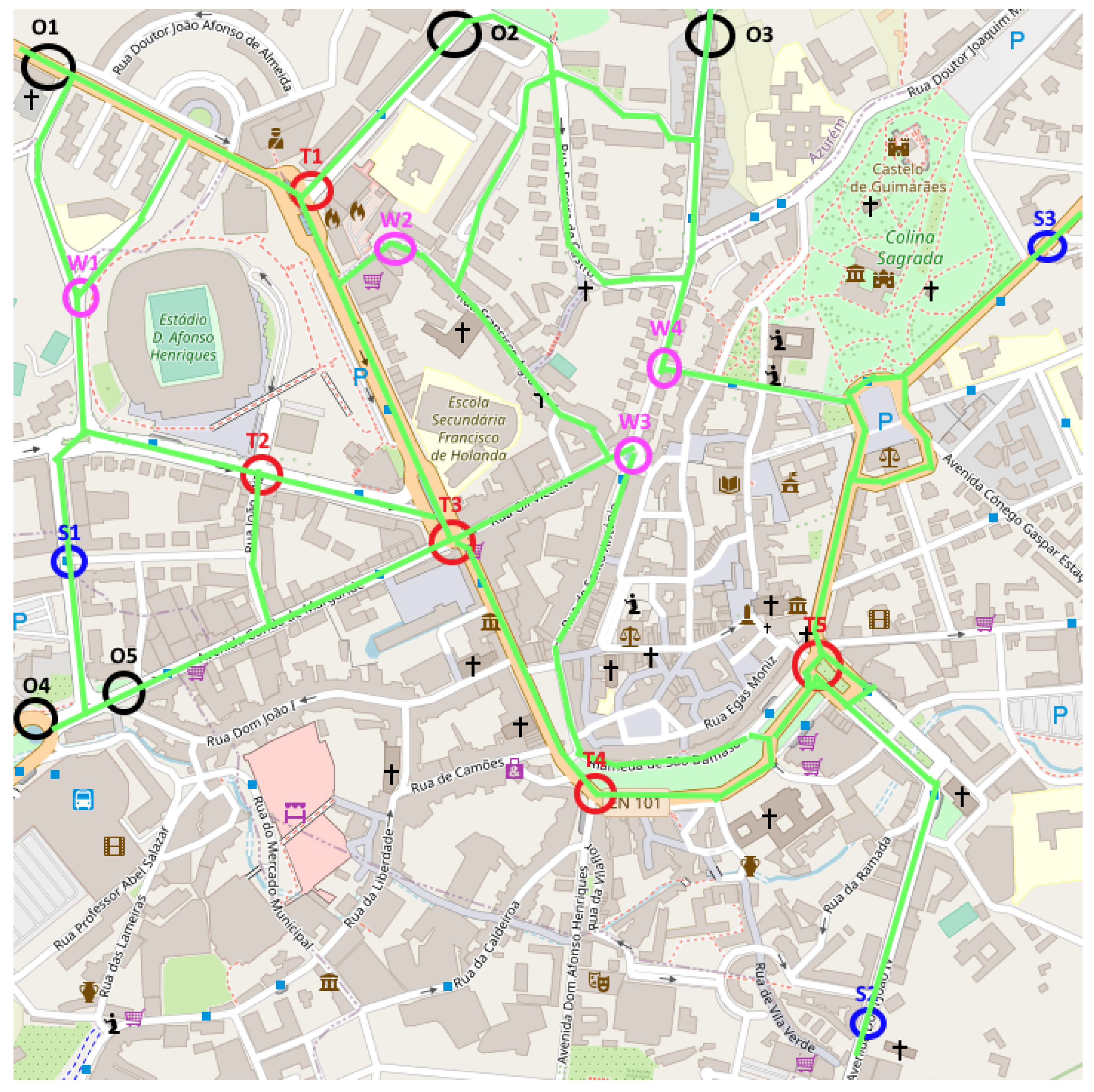
Figure 2 shows a map of the city center of Guimarães, the object of study of this work. The figure shows the area used for the replication of the real-world behavior, using red circles for traffic lights (T1, T2, T3, T4, and T5) and blue circles to show the positions of the sensors used to collect and measure the real-world traffic flows (S1, S2, and S3) within the city.

This work also includes real data taken from the traffic lights and buses. The data from the traffic lights were measured manually and introduced into the simulation; bus routes and departure times were collected from the city bus operator, Guimabus.

4.1. Traffic Data

Traffic data are one of the most important components in building a simulation scenario that can accurately replicate reality. For this work, real-world data were provided by the Guimarães City Hall. These data were obtained from sensors distributed across the city center (blue circles in Figure 2).

Table 1. Location of the sensors.

Sensor	GPS	Number of Sensors
S1	41.443271, −8.302675	2
S2	41.437777, −8.291246	2
S3	41.451333, −8.280557	2

presents additional information on these sensors, including their position and the number of sensors. All the locations have two sensors. Sensors S2 and S3 measure the traffic entering and leaving the city; both sensors in S1 measure the traffic in the same direction, as the street in this location has two lanes.

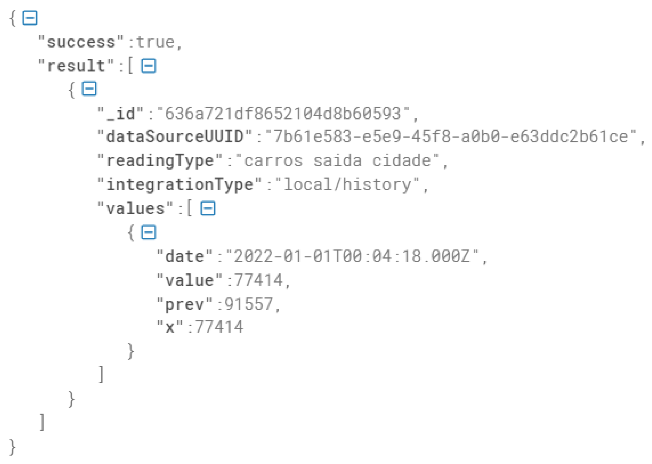
4.1.1. Data Records

Figure 3 shows an example of the collected data records. It shows four main fields date, value, prev, and x. These correspond to the sample date (date), the current number of vehicles that have passed through this particular sensor until the current time (value), the previous value before the current sample (prev), and the number of vehicles passing through the sensor (x); this last parameter (x) is 1 in the large majority of samples because a new sample is usually created each time a vehicle passes through the sensor.

The rest of the parameters, presented in JavaScript Object Notation (JSON), indicate the success of the operation, the sensor source ID, the type of information provided, and if it is real-time or historic (these are not of major importance for current work).

4.1.2. Data Fetching and Pre-Processing

The real-world data were provided and accessed through a Representational State Transfer (REST) Application Programming Interface (API) in JSON format. Manually fetching and organizing the data would be a very demanding job. Python is a simple and powerful scripting language, ideal for these situations. So, a script was coded using Python to iterate through the multiple sources and download the associated data. The script also filters the raw data, extracting only the traffic-related data. The data were then organized into multiple Comma Separated Value (CSV) files (according to each source). CSV is easily imported to other software, such as Excel, which provides data analysis tools.

Table 2. Sensors raw data.

Sensor	Way	Number of Samples	Avg Sample Time (s)	Standard Dev (s)	Total Time (Days)
S1	One-Way	94,556	16.41	162.57	18
S2	Way-In	191,516	11.71	5125.50	26
	Way-Out	105,132	21.33	126.88	25
S3	Way-In	644,132	14.98	83.44	111
	Way-Out	575,551	16.77	134.71	111

shows the attributes of the collected data, including the number of samples in each sensor, the average sample time, the standard deviation of the sample time, and the time interval in which the data point was collected.

Depending on the sensor, the data collection spanned between 18 days on sensor S3 to 111 days on sensor S1, obtaining a number of samples ranging from 94,556 entries to 644,132. Another important factor was the sample rate. As shown in Table 2, each collected data point does not have a constant sample rate. Instead, it has an entry for each time a vehicle passes through the sensor. Meaning that the intervals between each sample are not constant, and each interval only has one vehicle passing. This makes it hard to analyze. So, the next step was to resample the data, creating constant intervals. These allow for a better analysis of the collected data, providing insight into the traffic flow at each time instant.

The data re-sampling process consisted of grouping the data collected in a pre-determined period of time, in this case, 1 h, thus obtaining 24 time periods each day. This allows for the analysis of the traffic during each day’s period.

Table 3. Resampled Data (1 h intervals).

Sensor	Way	Samples	Average Flow Vehicles/Hour	Std Dev
S1	One-Way	431	232	200
S2	Way-In	939	157	130
	Way-Out	612	90	85
S3	Way-In	7967	103	194
	Way-Out	7967	210	180

contains the number of samples in each sensor that resulted from the re-sampling and average vehicle flow. In Section 5, a more in-depth analysis of the collected data is given.

5. Traffic Characterization

The goal of the data collection is to characterize the city traffic in order to create its virtual representation. This section describes the data collected in Section 4, including the vehicle data, traffic lights, and bus data.

5.1. Vehicle Data

The collected data spanned multiple days, ranging from 18 to 111 days (Table 2). Table 3 presents the average of the multiple traffic flows. However, this is of little relevance, as the traffic flow has huge variations during each day and between days, resulting in a high standard deviation. The same happens when averaging the traffic flow each day.

Table 4. Traffic flow average and standard deviation per weekday per sensor (vehicles/hour).

Sensor	Way	Sun	Mon	Tue	Wed	Thu	Fri	Sat	Std Dev
S1	One Way	170 ± 165	247 ± 209	210 ± 183	218 ± 192	237 ± 202	317 ± 587	231 ± 222	252
S2	Way-In	130 ± 116	167 ± 134	167 ± 136	167 ± 133	168 ± 135	182 ± 140	145 ± 118	130
	Way-Out	55 ± 51	98 ± 89	100 ± 95	91 ± 93	101 ± 96	110 ± 96	70 ± 61	82
S3	Way-In	188 ± 166	270 ± 220	270 ± 220	277 ± 220	279 ± 218	26 ± 187	259 ± 187	194
	Way-Out	116 ± 139	242 ± 232	245 ± 237	251 ± 236	256 ± 239	207 ± 103	201 ± 211	200

shows the average and standard deviation traffic flow for each day of the week. It can be seen that it still presents a high variance, with the standard deviation values having the same magnitude as the average. Additionally, the average standard deviation for each sensor is presented in the last column. These can range from 82 to 252 vehicles per hour on the sensors S2 and S1, respectively.

Table 5. Traffic flow standard deviation per day per sensor, averaged hour (vehicles/hour).

Sensor	Way	Sun	Mon	Tue	Wed	Thu	Fri	Sat	Average
S1	One Way	37	35	41	66	47	47	149	60
S2	Way-In	21	30	32	25	20	21	32	26
	Way-Out	15	30	34	30	23	22	27	26
S3	Way-In	51	63	59	55	45	90	54	60
	Way-Out	47	60	72	59	57	82	60	62

shows the standard deviation of the traffic flows per day of the way. However, the values in this table were calculated by averaging the traffic flow per hour of the day instead of the traffic flow per day, which has much better precision. The present table does not show the average for each hour due to the number of values needed. The goal was to show that using the traffic flow values average per day is of little use.

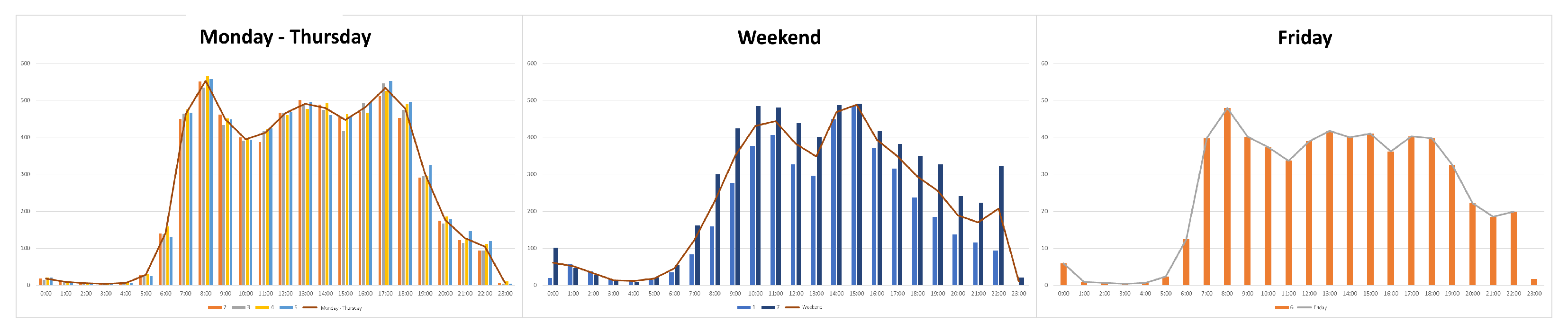
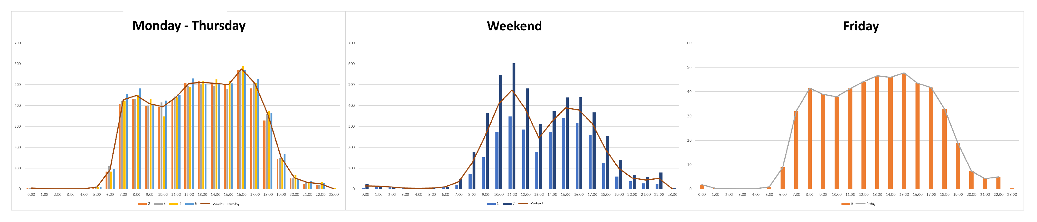
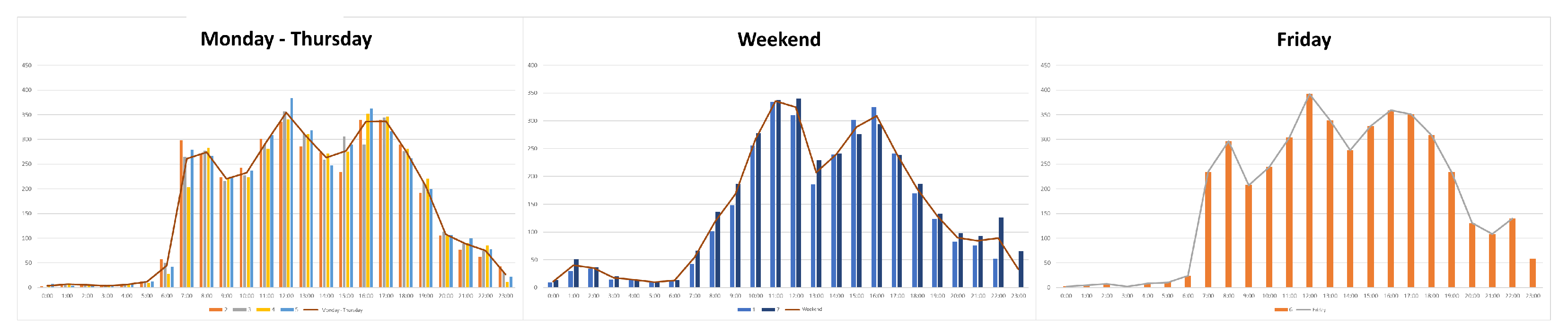
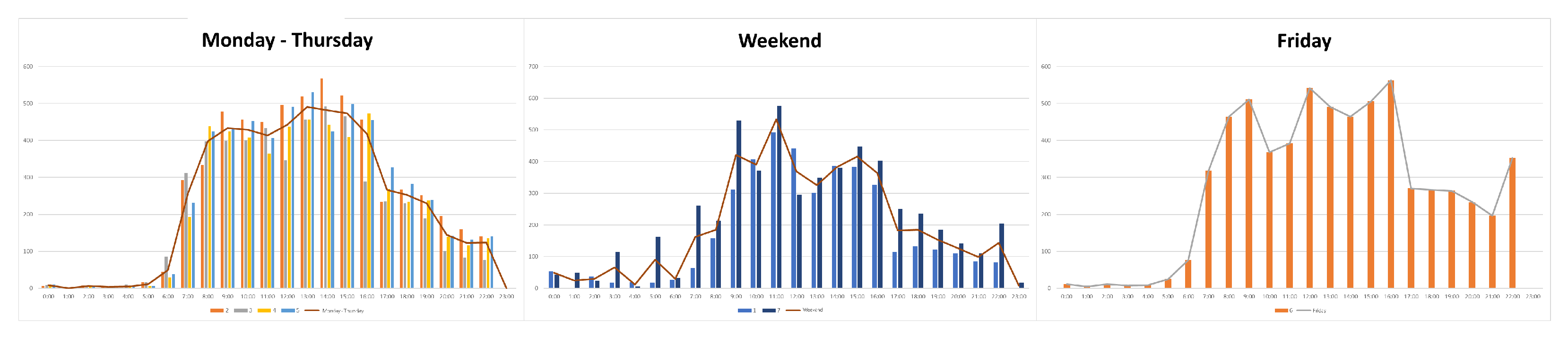
Figure 4, Figure 5, Figure 6, Figure 7 and Figure 8 show a comparison of the average traffic profiles—the average traffic flow per hour per day— in multiple sensors. Each of the figures presents three different charts. The first chart in each figure shows the traffic from Monday through Thursday, the second the traffic from Saturday and Sunday and the last Friday’s traffic. All traffic shows the average traffic during each hour on each day of the week. The line presented shows the average of all the values in each hour. These indicate that the traffic behavior is very similar during weekdays. The same happens on the weekends. Although some values are outside the average line, this line seems to represent quite well the traffic behavior. Friday seems to be an isolated case, having a general behavior different from the other two cases. Although this behavior may seem a little bit strange, it fits the observable behavior of road users. Usually, on Fridays, people’s movements are different from other work week days; with the weekend approaching, people leave work early, they go out shopping or eat out, creating different traffic patterns.

This behavior can serve to reduce the number of cases needed to accurately represent the traffic in the city on weekends, weekdays, and Fridays.

5.2. Bus Data

Public transportation is a vital part of urban cities, improving connectivity and allowing people to travel and reach their destinations. It is important to include them in the model for a more realistic representation of the traffic since buses are always circulating within cities, and bus stops can greatly impact traffic flow. The company GuimaBus (https://guimabus.pt/, accessed on 1 November 2023) is responsible for the collective passenger transport service in the municipality of Guimares, with a total of 66 bus routes comprising 1519 bus stops. However, only 24 bus routes (65 bus stops) are present in the selected region, and those were added to the model. Moreover, the bus fleet is 100% electrically powered. This information was collected from GuimaBus and is summarized in

Table 6. Bus routes used for simulation between 16:00 and 17:00 on a weekday.

Bus Route	Route Type	Bus Stops	N Buses	Departure Time (Bus Stop)
003	Circular	14	1	16:15 (128)
004	Circular	20	2	16:05 (624), 16:41 (624)
011	Round-trip	6	6	16:00 (794), 16:06 (498), 16:20 (794), 16:25 (498), 16:40 (794), 16:46 (498)
012	Circular	11	1	16:09 (498)
014	Circular	11	1	16:00 (2)
021	Round-trip	7	3	16:00 (794), 16:27 (474), 16:30 (794)
031	Circular	8	2	16:20 (710), 16:50 (710)
032	Circular	7	2	16:06 (624), 16:36 (624)
041	Circular	9	2	16:15 (715), 16:45 (715)
042	Circular	9	2	16:00 (715), 16:30 (715)
061	Circular	7	1	16:23 (474)
062	Circular	9	2	16:04 (1525), 16:34 (1525)
070	Circular	9	1	16:19 (613)
071	Circular	9	1	16:51 (2)
072	Circular	9	1	16:38 (613)
073	Circular	9	1	16:16 (2)
081	Round-trip	6	3	16:11 (2), 16:20 (999), 16:41 (2)
082	Circular	9	1	16:30 (715)
083	Circular	9	1	16:00 (715)
170	Round-trip	10	2	16:02 (554), 16:41 (710)

. In the table, the first column refers to the identifier for each route, and there are two types of routes: circular and round trip. Circular routes are routes that follow a circular shape (for example, around the city center), starting and ending at the same bus stop. On the other hand, round-trip routes consist of a more linear route (for example, from the city center to the city outskirts), and upon reaching the last bus stop, the bus turns around and returns to the initial bus stop.

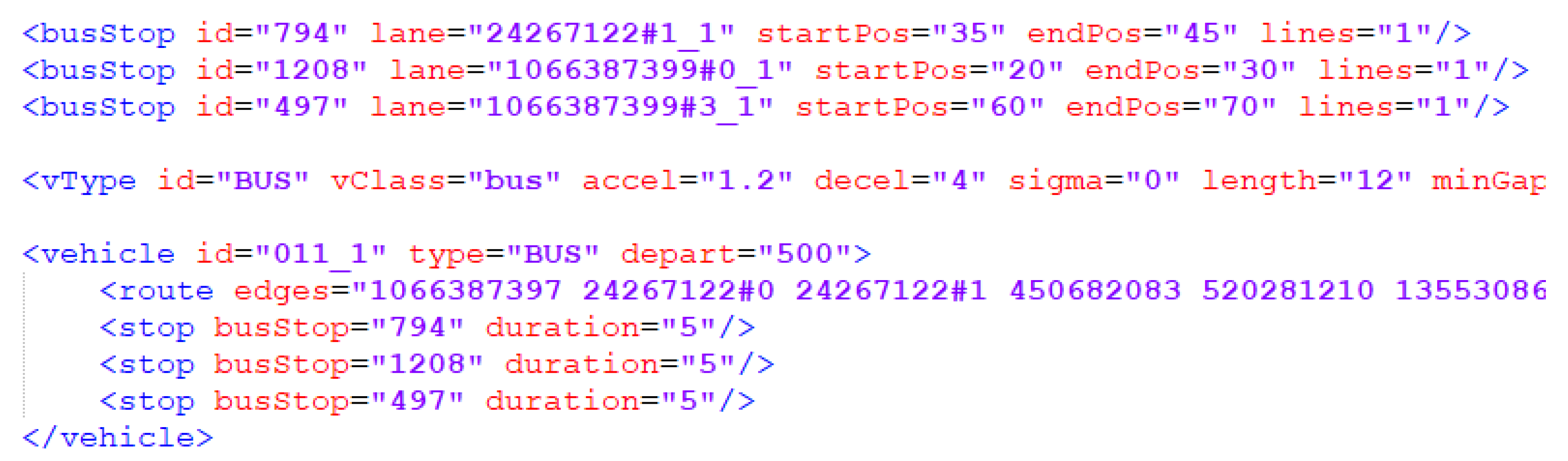
Bus stops and routes were coded in an $.xml$ file and added as an additional file to the SUMO configuration file. All buses have the SUMO default characteristics. To be coded, each bus stop needs an identification (in this case, its name), its location in the network (lane), and its position in the lane. The bus routes are the sequence of lanes (edges) in the network that the bus must follow. Figure 9 shows an example of the implementation of a bus circulating on its route. The departure time defines the trip’s start; while following its route, the bus stops at all defined stops.

5.3. Traffic Lights Data

In the selected area of the city center of Guimarães, Figure 2, there are five intersections, represented by T1, T2, T3, T4, and T5, where traffic lights regulate vehicles and pedestrian crosswalks. T1 is located in Rua Teixeira de Pascoais and controls two-way traffic to allow pedestrians to cross the road. T2 results from the intersection of two two-way streets with multiple lanes, Av. São Gonçalo and Rua João XXI; therefore, there is one traffic light regulating the traffic for each direction and the corresponding crosswalks. The intersection T3 involves five one-way streets with different numbers of lanes, Av. Conde de Margaride, Alameda Dr Alfredo Pimenta, Av. São Gonçalo, Rua de Gil Vicente, and Rua Paio Galvão. This intersection is one of the points where traffic becomes congested due to a high number of pedestrians crossing the road coming from the nearby school Escola Secundária Francisco de Holanda. Through this intersection, it is also possible to access the historic city center. Traffic circulating on Alameda de São Dâmaso (two-way street) has the option to turn onto the Av. Dom Afonso Henriques (one-way only) at T4. To regulate this intersection, there are traffic lights. T5 is a roundabout named Largo da República do Brasil where traffic lights are used on two different roads that converge into the roundabout. Two traffic lights regulate the traffic entering and exiting the Alameda de São Dâmaso, and two other traffic lights similarly regulate traffic on Av. Alberto Sampaio. In total, there are 18 traffic lights in this region.

The real traffic light cycle was measured on-site, resulting in the cycle times shown in

Table 7. Traffic light cycle times measured.

Intersection	Total Cycle Time (s)
T1	41
T2	119
T3	89
T4	72
T5	41

. At intersections T4 and T5, the fixed cycle can be interrupted when pedestrians press the button to cross the road. This made it difficult to measure the cycle times of the traffic light accurately, and an average time from several measurements was used in this case.

Every traffic light cycle, within two green light periods, has a 3-second yellow light followed by a 3-second red light to ensure that vehicles slow down and stop safely and that intersections are clear before the next green light. Each cycle also has a 15-second red light phase for vehicles so pedestrians can cross the road safely.

6. Replication of Real-World Traffic

The replication of real-world traffic in a chosen location needs multiple steps. First is the definition of the geographical real-world area to be simulated. Using the defined bounds, it is then possible to create the scenario in simulation using parameters and roads imported directly from a real location (Section 6.1). Then, it is possible to carefully define the routes that the vehicles in the simulation will follow, complying with real-world traffic laws and trying to represent the real routes in the city (Section 6.3). The next step is the definition of the traffic flows (Section 6.2), which indicate how many vehicles should travel on each route in the period of one hour. These flows can be computed from the real-world data collected in Section 4. The final step is the simulation of the defined scenario using a simulation framework (Section 6.4).

This simulation scenario, based upon real city traffic data, is also planned to establish a baseline for traffic optimization studies within the city. This will be accomplished either by analyzing and defining strategies to optimize the traffic light cycle times of several intersections and crossroads—an ongoing study using this urban simulation platform (using the U-NSGA-III optimization algorithm [27]) is already underway—or by analyzing several traffic diversion alternatives taking into account the Braess Paradox [28]. This is a counter-intuitive fact that the creation of shortcuts may complicate traffic flows and can lead to increased average travel times for all users [29].

6.1. Scenario Creation

Creating a scenario for simulating a realistic scenario in MOSAIC involves several steps. These are described below and illustrated in the workflow.

(1) First of all, it is necessary to define the geographical area. This is a set of coordinates that constitute a quadrilateral geometric figure. The selected area must accommodate the entire real-world area to be studied. In this particular case, the rectangle has the coordinates 41.4493 −8.3034, 41.4371 −8.2865.

(2) Using the defined area, the map can be obtained. OpenStreetMaps (OSM) is an online platform that provides maps for free in an open-source format. This format can then be easily imported into SUMO and MOSAIC.

(3) Import the maps obtained from OpenStreetMaps into MOSAIC. MOSAIC provides scenario-convert, a tool to convert OSM maps to MOSAIC scenarios. In this case, if it is used with the “–osm2mosaic” option, it will automatically create all the necessary files and file structures for MOSAIC.

(4) Create the route files for SUMO. These are the files that define the route of each vehicle on the map. These can also be created using scenario-convert.

6.2. Traffic Flows

The available real-world data provide accurate information about the traffic at several locations in the city center of Guimarães. Unfortunately, the sensors that provide the data are located at only three different places. Thus, while the data alone may not be sufficient to accurately represent the traffic at other locations of the city center, they can be used to infer the traffic flow at unrepresented locations. So, the traffic flows on each major downtown road can be calculated according to three methodologies:

• A—Traffic flow values collected by the sensors;
• B—Traffic flows required at unrepresented locations for the known values to be correct;
• C—Values inferred through real-world knowledge.

A is the easiest way to calculate the traffic flow; it directly uses the values measured by the traffic sensors. However, this methodology needs to be used in conjunction with the other measures. Although indicating the traffic flow in each direction at the specific location, the sensor data do not clearly identify the origin and destination of the traffic. This has to be inferred using both methods A and B.

Method B uses the values from A. In this methodology, the values of all the sensors are used in conjunction. As mentioned before, the values of the sensors do not indicate the origin and destination of the traffic. By using the values of the multiple sensors together, it is possible to know the origin and destination of traffic and the traffic that will exceed these values. This excess traffic will then be used in method C.

Method C uses the traffic in excess in combination with practical knowledge of the city to infer the traffic at these locations. Since this is real-world knowledge of the city, the precise values are unknown; however, comparative values can be inferred.

Even though any of the methods may not be exact, the combination of all of them can accurately describe the city traffic. During the simulation design and establishment of the traffic flows, it was noticed that an equilibrium was needed to obtain the desired traffic flow values at each known point. The traffic flow at each point is self-verifiable because every traffic flow affects the others. So, if the traffic flow at a point is increased, it will affect others by creating jams or allowing and stopping the needed flow for other pairs’ origin–destinations. For example, increasing the traffic flow from S3 to S1 can easily overwhelm the connection at T5, preventing the correct flow from S2 to O1, O2 or O4.

Since all previously defined methods are needed to recreate the traffic accurately, the flows at each origin were defined by trial and error to approximate the known values.

6.3. SUMO Routes

As mentioned, the traffic simulation in the presented work was carried out through SUMO. SUMO has multiple ways of defining traffic flows. However, MOSAIC only supports the definition of the traffic flows through routes. More precisely, MOSAIC uses the route files to define the flow on each route (MOSAIC supports other flow creation methodologies; this one, however, allows more control over the flows).

Because of the known traffic flows at the sensor locations, these were all used as either traffic waypoints (S1) or as start or end points of the traffic flow (S2 and S3). Additionally, due to their importance in the traffic flow in the actual city, other points were defined to serve as traffic start and endpoints. These new points are shown on the map as O1, O2, O3, and O4. These are high-flow points composed of the University of Minho (O2 and O3), the shopping mall (O4 and O5), and the route to the nearest city, Braga (O1). The points indicated as W1 to W4 are auxiliary points inserted to better characterize the created routes (shown in

Table 8. SUMO Routes.

Route	Origin	Waypoint	Destination
1	S3	W4, W2, T1	O2
2	S3	T5, W3, T3, T1	O2
3	S3	T5, W3, T3	O1
4	S3	T5	S2
5	S3	T5, W3, T3, T2, S1	O4
6	S2	T5	S3
7	S2	W4, W2, T1	O2
8	S2	T5, W3, T3, T1	O2
9	S2	T5, W3, T3, T2, S1	O4
10	O5	T3, T4, T5, S3	S3
11	O5	T3, T1	O2
12	O5	T2, W1	O1
13	O5	T3, T1	O1
14	O1	O2, W4	S3
15	O1	T3, T4, T5	S3
16	O1	T1	O2
17	O1	W1, S1	O4
18	O1	T3, T4, T5	S2
19	O2	T1	O1
20	O2	T1, W1, S1	O4
21	O2	T1, T3, T2, S1	O4
22	O1	W4, T5	S2
23	O2	T1, T3, T4, T5	S2
24	O2	W4	S3
25	O2	T1, T3, T4, T5	S3
26	O5	T3, T4, T5	S2
27	S3	W4	O3

). In Figure 10, the updated map with the new points is shown. In addition, the streets through which traffic flows are shown.

Both the university and the shopping mall need two points as origin and destination because of the city traffic flows. O3, O4, and O5 only allow one-way traffic. O2 and O3 are both needed because they are two traffic routes used to access the university.

These routes were also created using scenario-convert provided by MOSAIC. This tool can create routes in multiple ways. However, the one that gives the most control receives the start and end points as input and creates the desired number of alternative routes. Using this methodology, 27 routes were created. These are presented in Table 8, indicating the SUMO route, the origin, the destination, and one other point for easy identification.

6.4. Eclipse MOSAIC Mapping

MOSAIC provides a methodology to easily use the routes defined in SUMO. This can be accomplished through a mapping file. This file allows for linking vehicles with a desired route, indicating the target traffic flow on each route. Moreover, it is possible to define which types of vehicles should circulate on each route. Additionally, and if necessary, the mapping file allows one to attribute a Java application to a vehicle (or any other entity), giving it a panoply of new functionalities.

A realistic scenario has multiple vehicles with different sizes and movement characteristics.

Table 9. Vehicle type distribution. (* vehicles added directly in SUMO).

Name	Vehicle Class	Weight
Car	Car	0.4
Bus	Public Transport Vehicle	*
Heavy Goods	Heavy Goods Vehicle	0.01
Light Goods	Light Goods Vehicle	0.1
Works Vehicle	Works Vehicle	0.1
Taxi	Taxi	0.19
Bicycle	Bicycle	0.07
Motorcycle	Motorcycle	0.19
High Occupancy Vehicle	High Ocupance Vehicle	0.05

shows the types of vehicles used and the percentage of each preset in the simulation. So, as it indicates, the most common vehicle is a passenger vehicle, followed by motorcycles and taxis. The least common is the heavy goods vehicle, as there seems to be a low probability of them passing through the city. Table 9 shows bus weight as “*” because buses are introduced directly into the simulation through SUMO, without the MOSAIC mapping file, following the route patterns presented in Section 5.2.

The creation of the MOSAIC mapping file and, consequently, the completion of the simulation scenario needs to match the targeted traffic flows at each map point previously indicated (blue circle), since these values represent the real-world count. In this work, it was chosen to select the time of day with the highest traffic. Thus, the solution would be to analyze the values shown in Figure 4, Figure 5, Figure 6, Figure 7 and Figure 8 and choose the most representative one, containing the heaviest traffic either entering or exiting the city. The results presented and discussed were taken from simulation runs encompassing one hour of heavy traffic flows; this period seems to occur from 16h00 to 17h00 on weekdays, from Monday to Thursday. The traffic flows for the selected period are shown in

Table 10. Selected traffic flows.

Sensor	Way	Traffic Flow (Vehicles/Hour)
S1	One Way	447
S2	Way-In	478
S2	Way-Out	573
S3	Way-In	358
S3	Way-Out	180

.

Table 11. Mapping target flows (vehicles/hour).

Route	1	2	3	4	5	6	7	8	9
Target Flow	-	50	50	20	53	150	-	210	110
Route	10	11	12	13	14	15	16	17	18
Target Flow	5	230	175	150	25	-	120	205	190
Route	19	20	21	22	23	24	25	26	27
Target Flow	230	90	90	30	160	-	-	310	235

combines the values presented in Table 8 and Table 9, showing the target flow for each route. The goal of the values in these tables was for the simulation values to be as close as possible to the values in Table 10. The results obtained are shown in Section 7. During the process of creating the traffic flows on each route, some of the existing routes were not used. This usually happened because the traffic on those routes interfered with other routes, preventing the flows from reaching the goal values.

7. Results and Discussion

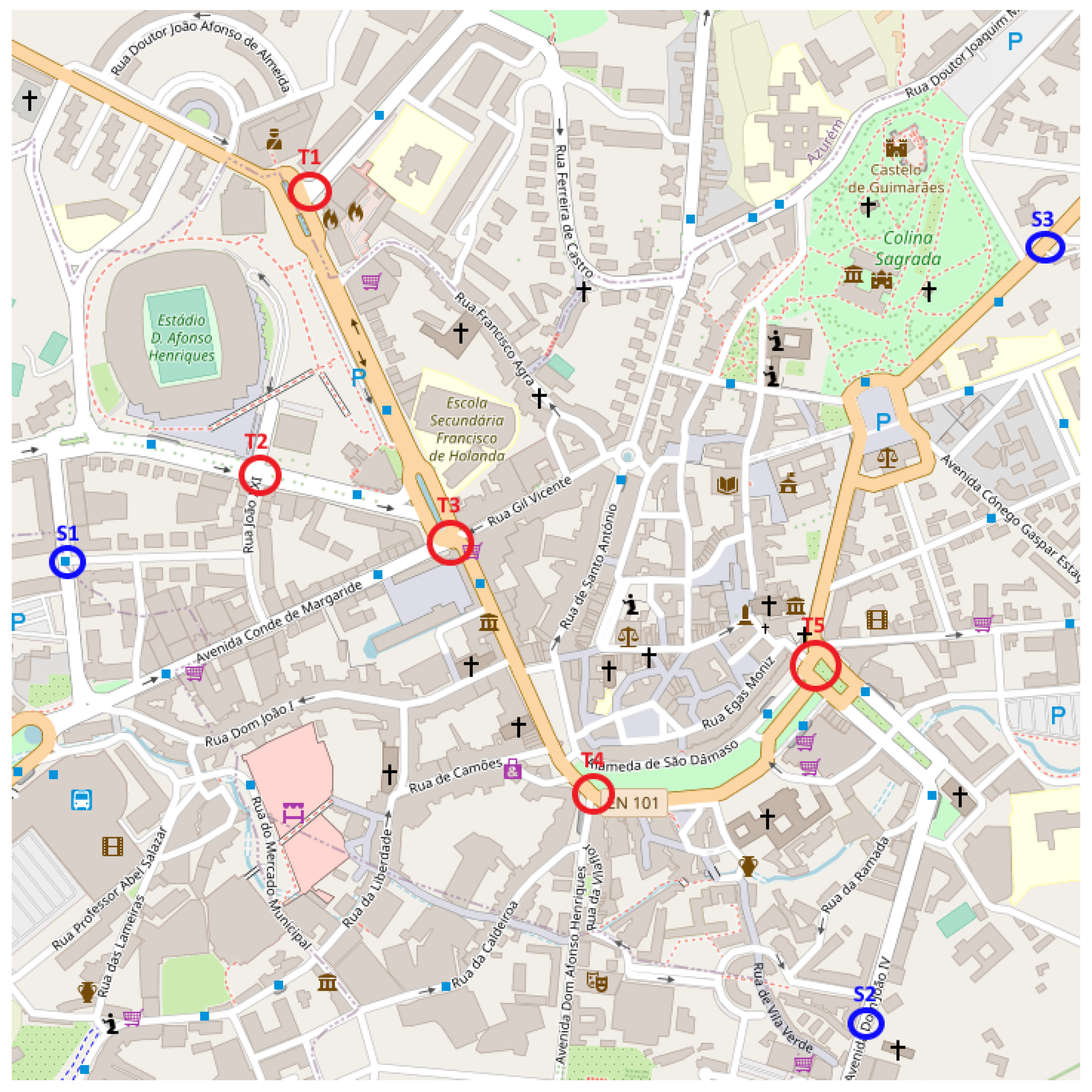
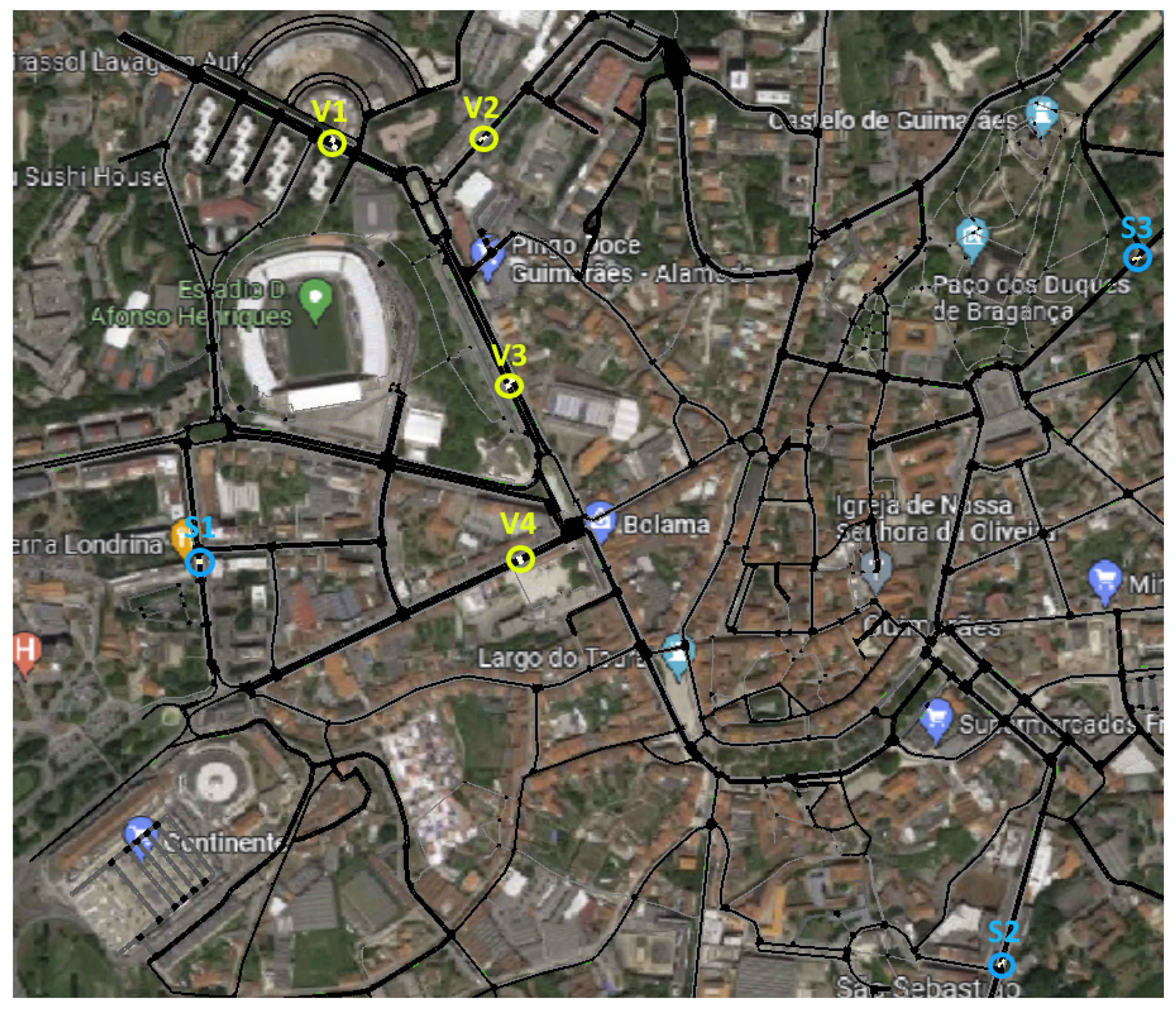
Using the configurations defined in the previous sections, a simulation scenario was established, using SUMO as the traffic simulator and MOSAIC Eclipse for extended capabilities, such as applications to run on the traffic management system (road sensors) and on the vehicles to store the driving data. Figure 11 shows an updated view of the simulation area. This is what can be seen in SUMO when running the simulation. In reality, it results from an overlay of a Google Maps screenshot over the SUMO graphical interface. Additionally, in Figure 11 the locations of the sensors from which the data were collected are shown in blue (similarly to Figure 2) and four extra points, shown in yellow (V1, V2, V3, and V4), are virtual traffic sensors added to the simulation in order to obtain traffic counts, which enable a better analysis of the created traffic flows. The location and number of virtual traffic sensors can be seen in

Table 12. Location of the virtual sensors.

Sensor	Location	Number of Sensors
V1	41.447942, −8.300653	2 + 2
V2	41.448006, −8.298386	1 + 1
V3	41.445357, −8.298120	2 + 2
V4	41.443308, −8.298012	3

. The columns in the table indicate the sensor name, their GPS locations, and the sensor number at each location. The values shown as x + y represent the number of sensors in each location.

The results obtained from the simulation are presented in

Table 13. Traffic flows obtained from the simulation (Grey row indicates the total for each sensor).

Sensor	Way	Lane	Traffic Flow (Vehicles/Hour)
S1	-	1	405
	-	2	35
		Tot	440
S2	Way-In	1	477
	Way-Out	1	572
S3	Way-In	1	358
	Way-Out	1	181
V1	O - E	1	244
	O - E	2	106
		Tot	350
	E - O	1	181
	E - O	2	157
		Tot	338
V2	N - S	1	473
	S - N	1	394
V3	O - E	1	368
	O - E	2	6
		Tot	374
	E - O	1	336
	E - O	2	137
		Tot	547
V4	-	1	127
	-	2	242
	-	3	209
		Tot	548

, which indicates the flow obtained at each sensor at each location. The first column shows the sensor’s name, followed by the direction of the traffic it is measuring (if there is more than one way) and the lane. In the last column, the sum of the flows at all the sensors in the same direction is shown. The flow indicates the number of vehicles that passed through each sensor during the one-hour period. This shows the traffic flows obtained at each traffic sensor (virtual and real). The lanes used by the vehicles are selected by the simulator. This results in the uneven distribution of the vehicles per lane, creating situations such as lane 2 of sensor V3, where there are no vehicles during all simulations. Since one of the lanes is sufficient for all the traffic crossing it, the simulator chose to use only one of the lanes for almost all the traffic, with only a few vehicles in the other one.

The values obtained from the simulation can be compared with those collected from the real world (see Table 10). The result is a scenario very close to reality, with a difference of a few vehicles per hour at each sensor. Moreover, although the values at these particular locations are not available, the values obtained with the virtual sensors seem to be acceptable, based on the real-world knowledge of the city and its comparison with the known values. For example, V4 is one of the city locations with the highest traffic. This fact is confirmed by the results obtained. The other sensors present values of the same order of magnitude, which also seems reasonable since they are all placed in heavy-traffic locations.

Table 14. Simulation results.

Routes	Vehicles	Fuel (mL/km)	CO2 (mg/km)	Distance (m)	Stopped Time (s)	Stopped Time (s/km)
1	-	-	-	-	-	-
2	33	0.47	1106	2486	258	1.03
3	34	0.36	844	2603	200	0.77
4	17	0.20	466	1458	23	0.16
5	-	-	-	-	0	-
6	141	0.18	426	1499	2	0.01
7	-	-	-	-	-	-
8	139	0.43	1014	2548	248	0.97
9	79	0.36	846	2783	268	0.96
10	4	0.23	535	2076	161	0.77
11	134	0.71	1651	1308	304	2.32
12	112	0.55	1270	1349	338	2.27
13	87	0.58	1341	1425	324	2.27
14	22	0.17	405	2204	2	0.01
15	-	-	-	-	-	-
16	113	0.17	388	770	2	0.03
17	192	0.15	350	1000	$>1$	>0.01
18	178	0.24	570	2291	95	0.42
19	149	0.54	1268	742	63	0.85
20	58	0.35	806	1544	63	0.41
21	59	0.39	920	1646	144	0.09
22	18	0.17	404	1939	35	0.18
23	103	0.36	833	2270	157	0.69
24	-	-	-	-	-	-
25	-	-	-	-	-	-
26	218	0.32	736	1933	153	0.79
27	220	0.17	402	1051	-	0.00
Total Avg	2110	0.34	790	1608	143	0.08

shows multiple metrics that were obtained from the filtered simulation by each route and the average per simulation. These indicate the number of vehicles per route and then the averages of fuel spent by each vehicle, the produced CO₂, the distance traveled by each vehicle, and the amount of time each vehicle was stopped. Moreover, it also presents the value for the stopped time per km; otherwise, scenarios with longer roads could seem to have unfairly higher stopped times due to their longer roads. All metrics were obtained directly from SUMO, including the values of the emissions. SUMO uses the different defined vehicle classes to try to give an accurate estimate of the emissions produced.

Although all these metrics can be valuable for studying the environmental impact of traffic, the time stopped is particularly interesting. This indicates the amount of time a vehicle is stopped during its trip. Ideally, this value would be 0, meaning that the vehicle could travel the entire route without stopping, either due to traffic or traffic lights. Thus, it is particularly important to measure the efficiency of traffic rules in a city. It can be combined with the emissions and vehicle consumption to produce a result that would balance traffic efficiency with emissions. The last line of the table shows the total average of the vehicles in the simulation. This was calculated from the raw data and not on the individual values of the table.

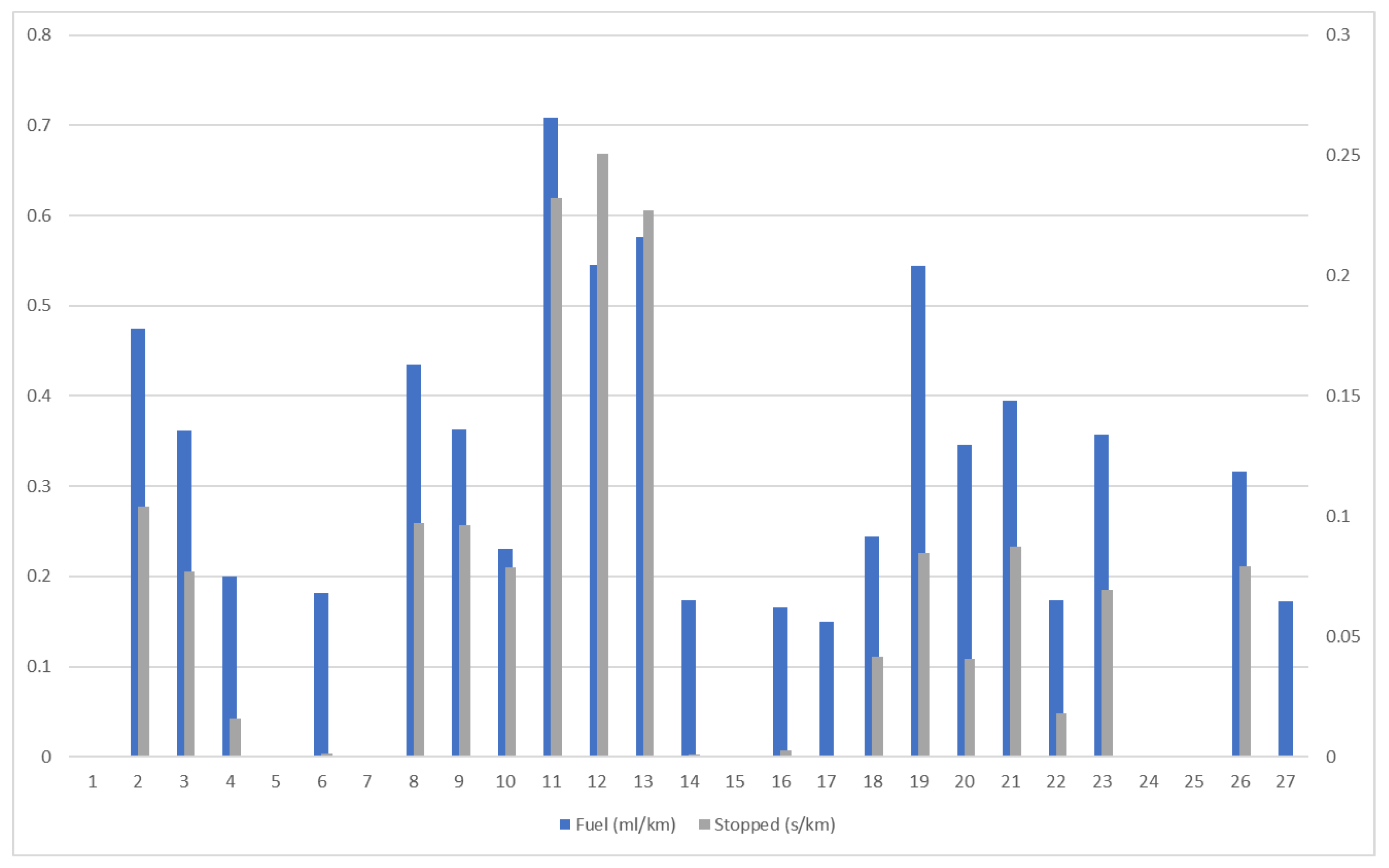
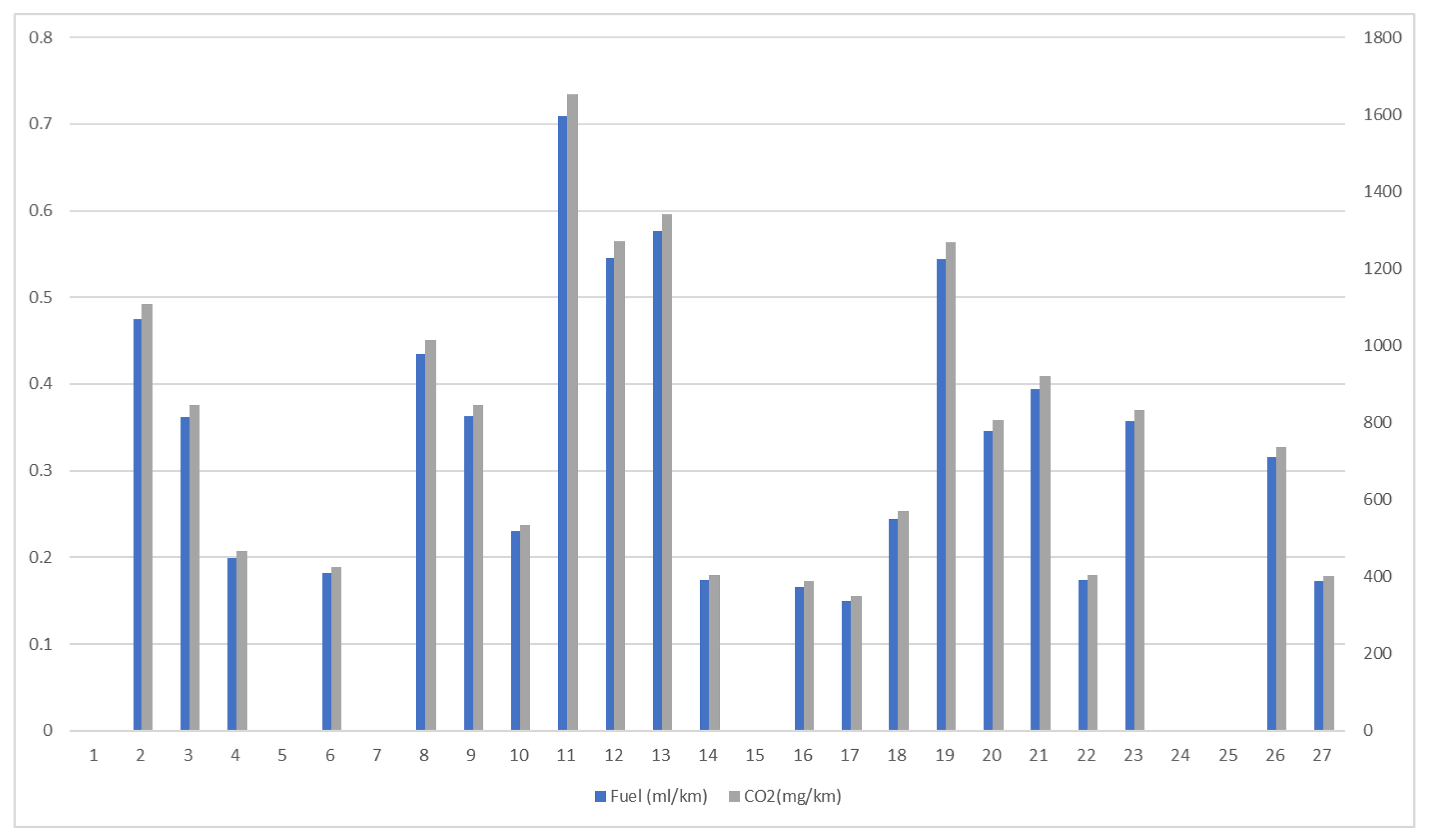
These results are particularly noticeable in Figure 12. This chart shows how the emissions and fuel consumption relate to each other. The chart shown has two different scales to accommodate the different magnitudes of the values presented. The values from CO₂ emissions use the scale indicated in the left-most scale (0 to 4000), and the fuel is represented in the right-most scale (0 to 0.8). It can be seen that, as expected, the vehicles that consume more fuel also produce more emissions (e.g., route 2).

In Figure 13, the values of the fuel consumption and the stopped time are compared. These results indicate that the vehicles must be using fuel while stopped. Thus, the scenarios with longer stopped times per km are the ones with more fuel consumption. Furthermore, this indicates that traffic optimization may be critical in order to minimize stopped time and, consequently, fuel waste.

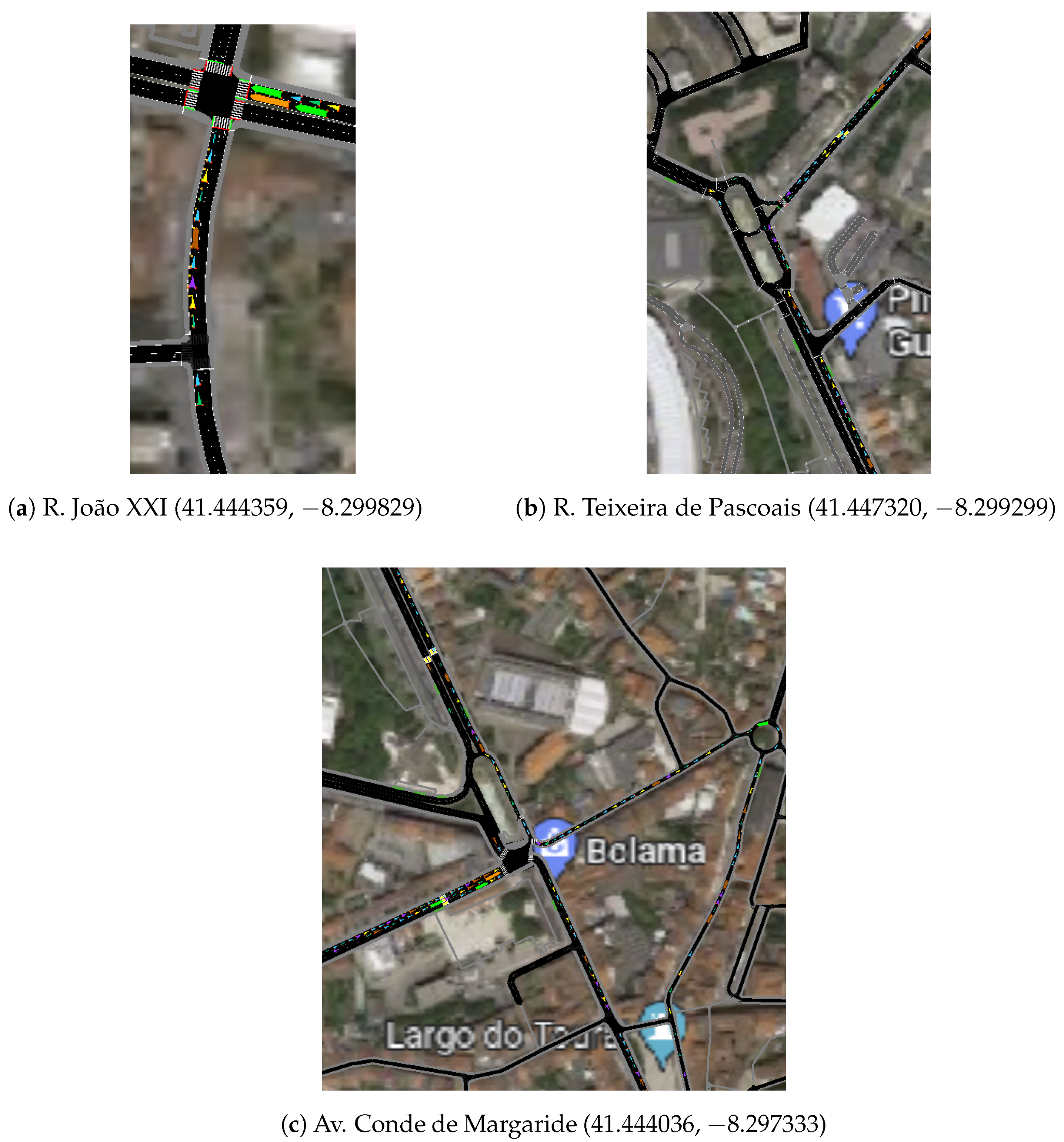
Another simulation result is the visual representation of the traffic. Figure 14a–c show the traffic created in the simulation. It can be easily seen that the traffic creates heavy traffic in multiple locations, which is deduced by the stopped times shown in Table 14. The results show that the traffic is inefficient, creating slow traffic in multiple routes, where vehicles need to stop multiple times along their route. This may happen due to multiple reasons, including too many vehicles on a specific stretch of road or ill-set traffic light times. So, the traffic could probably be optimized, either by redirecting vehicles (which could cause other problems [28]) or adjusting the traffic lights [12,30].

8. Conclusions and Future Work

This work presents the replication of real-world traffic in the city center of Guimarães, using data collected from real sensors, providing an accurate view. The data collected from the real-world traffic sensors were then analyzed, evaluating the traffic behavior and allowing a selected time period to be simulated.

The locations of the sensors were not enough to fully characterize the traffic in the city, and through a combination of data and real-world knowledge, the origin–destination matrix was defined, resulting in 27 vehicle routes. Additionally, virtual sensors were deployed during the simulation to count the traffic at critical locations, allowing for a better understanding of the traffic flows.

Moreover, the simulation allowed for a way to gauge the fuel consumption and emissions of the vehicles inside a city. Furthermore, it showed how traffic inefficiency can increase these metrics due to unnecessary stopped time. The next step would be to use optimization algorithms to reduce this stopped time and evaluate its impact on the vehicle’s fuel consumption and emissions.

Furthermore, the coupling of the traffic and network simulator through a simulation framework enables one to easily extend the resulting solution into more complex simulations that can take advantage of the bi-directional communication.

The results show that the created simulation scenario can accurately replicate reality, being a good basis for future research work, enabling the usage of unbiased datasets and traffic scenarios. The data collected and simulation scenarios, as well as the applications, were all made available at https://doi.org/10.5281/zenodo.7997433 and https://github.com/fabio-r-goncalves/norte (accessed on 1 November 2023).

The next goal is to create other traffic patterns to simulate different time periods and model a simulation encompassing a whole day. Additionally, it would be ideal to introduce more sensors in the city, starting with the locations where virtual sensors were used, to create a more accurate simulation.

As previously mentioned, the major limitation of the work is the lack of more physical sensors in other locations that could give a more accurate view of reality. Also, the obtained data were unbalanced, with more data from sensors from some locations, which could cause some bias in the final results.