VGG-C Transform Model with Batch Normalization to Predict Alzheimer’s Disease through MRI Dataset

Abstract

Alzheimer’s disease is the most common cause of dementia and is a generic term for memory and other cognitive abilities that are severe enough to interfere with daily life. In this paper, we propose an improved prediction method for Alzheimer’s disease using a quantization method that transforms the MRI data set using a VGG-C Transform model and a convolutional neural network (CNN) consisting of batch normalization. MRI image data of Alzheimer’s disease are not fully disclosed to general research because it is data from real patients. So, we had to find a solution that could maximize the core functionality in a limited image. In other words, since it is necessary to adjust the interval, which is an important feature of MRI color information, rather than expressing the brain shape, the brain texture dataset was modified in the quantized pixel intensity method. We also use the VGG family, where the VGG-C Transform model with bundle normalization added to the VGG-C model performed the best with a test accuracy of about 0.9800. However, since MRI images are 208 × 176 pixels, conversion to 224 × 224 pixels may result in distortion and loss of pixel information. To address this, the proposed VGG model-based architecture can be trained while maintaining the original MRI size. As a result, we were able to obtain a prediction accuracy of 98% and the AUC score increased by up to 1.19%, compared to the normal MRI image data set. It is expected that our study will be helpful in predicting Alzheimer’s disease using the MRI dataset.

1. Introduction

Alzheimer’s disease is the most common stage of dementia, requiring extensive medical attention. Early and precise analysis of AD prediction is required for initiation of clinical progression and effective patient treatment [1]. AD is a chronic neurobiological brain disorder that continuously kills brain cells and causes deficits in memory and thinking skills, eventually accelerating the loss of the ability to perform even the most basic tasks [2]. In the early stages of AD, doctors use neuroimaging and computer-aided diagnostic approaches to classify the disease. According to the World Alzheimer’s Association’s most recent census, more than 4.7 million people over the age of 65 in the United States have survived the disease [3]. The report also predicts that around 60 million people will be affected by AD within the next 50 years. Worldwide, AD accounts for about 60–80% of all forms of dementia, and there is a 60% chance that one dementia patient every 3 s, due to AD [4]. Alzheimer’s dementia is divided into:

-

Mild cognitive impairment: while generally affected by a memory deficit in many people as they age, in others it leads to problems with dementia.

-

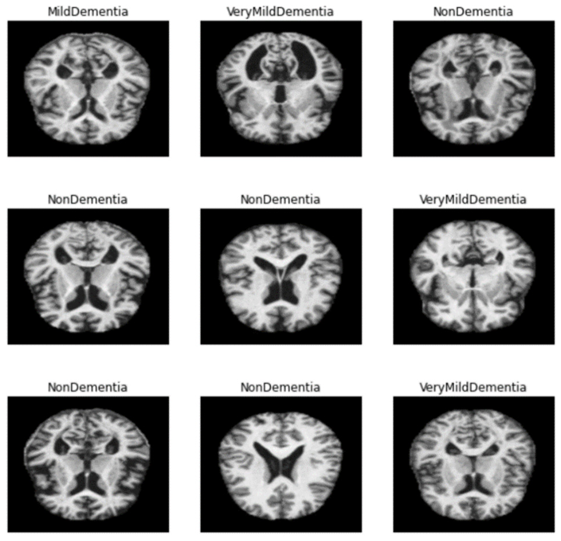
Mild dementia: Cognitive impairment that sometimes affects their daily life is found in people with moderate dementia. Symptoms include memory deficits, uncertainty, personality changes, feelings of loss, and difficulty performing daily tasks.

-

Moderate dementia: daily life becomes much more complex, and patients require special care and support. Symptoms are comparable to mild dementia but somehow get worse. People may need more help, even combing their hair. They can also show significant personality changes; for example, they become paranoid or irritable for no reason. Sleep disturbances are also likely to occur.

-

Severe Dementia: At this stage, symptoms may worsen. These patients may lack communication skills and may require full-time treatment. The bladder can’t be controlled, and you can’t do small activities, such as sitting in a chair with your head raised and maintaining a normal posture. Various research paradises have been conducted to slow the abnormal degeneration of the brain, reduce medical expenses, and improve treatment. According to nih.gov’s “Alzheimer’s Disease Fact Sheet”, the failure of recent AD research studies may suggest that early intervention and diagnosis may be important for the effectiveness of treatment [5]. Various neuroimaging methods are increasingly reliant on early diagnosis of dementia, which is reflected in many new diagnostic criteria. Neuroimaging uses machine learning to increase diagnostic accuracy for various subtypes of dementia [6].

Implementing a machine learning algorithm requires specific preprocessing steps. Feature extraction and selection, feature dimension reduction, and classifier algorithms are all steps in the machine learning-based classification process [7]. These techniques require advanced knowledge and several optimization steps, which can be time consuming. Recently, early detection and automatic AD classification [8] have emerged, resulting in large-scale multimodal neuroimaging results. Other methods of AD research include MRI, positron emission tomography (PET), and genotype sequencing results. Analyzing different modalities to make a decision is time consuming. In addition, patients may experience radioactive effects with modalities, such as PET [9]. It is considered important to develop better computer-aided diagnostic systems that can interpret MRI [10] images to identify patients with AD. Existing deep learning systems use cortical surfaces to input CNNs to perform AD classification on raw MRI images [11].

The important contributions of this study are:

• As mentioned above, the method of diagnosing AD on MRI images compares the size of the hippocampus. However, due to the nature of the existing CNN model, it is difficult to detect because it is not sensitive to image dispersion. Therefore, additional processing of the color space of the image is required.
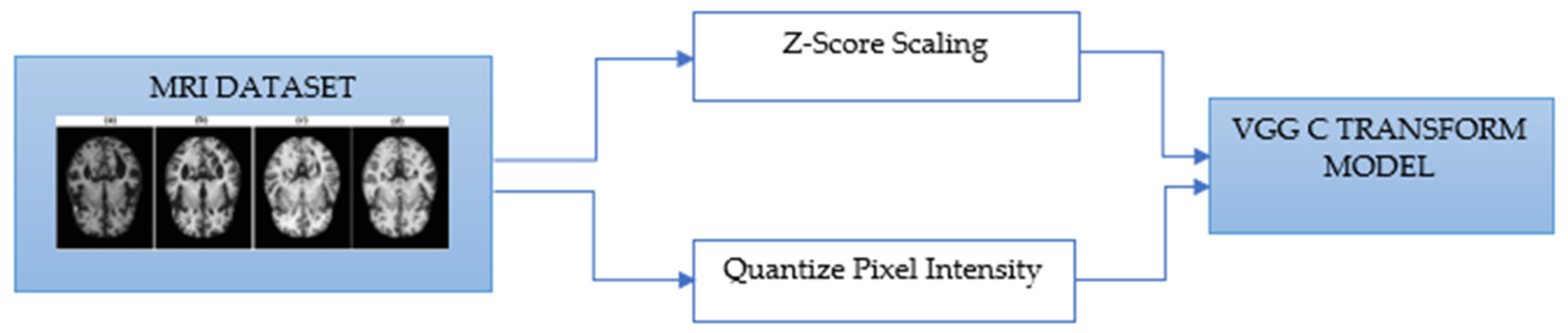
• For Z-score normalization, the interval to which each pixel belongs is converted to [−1, 1], and for min–max, it is converted to [0, 1]. During the computation of the convolutional neural network, the pixel intensity of [0, 255] is adjusted for fast convergence and accurate feature extraction.
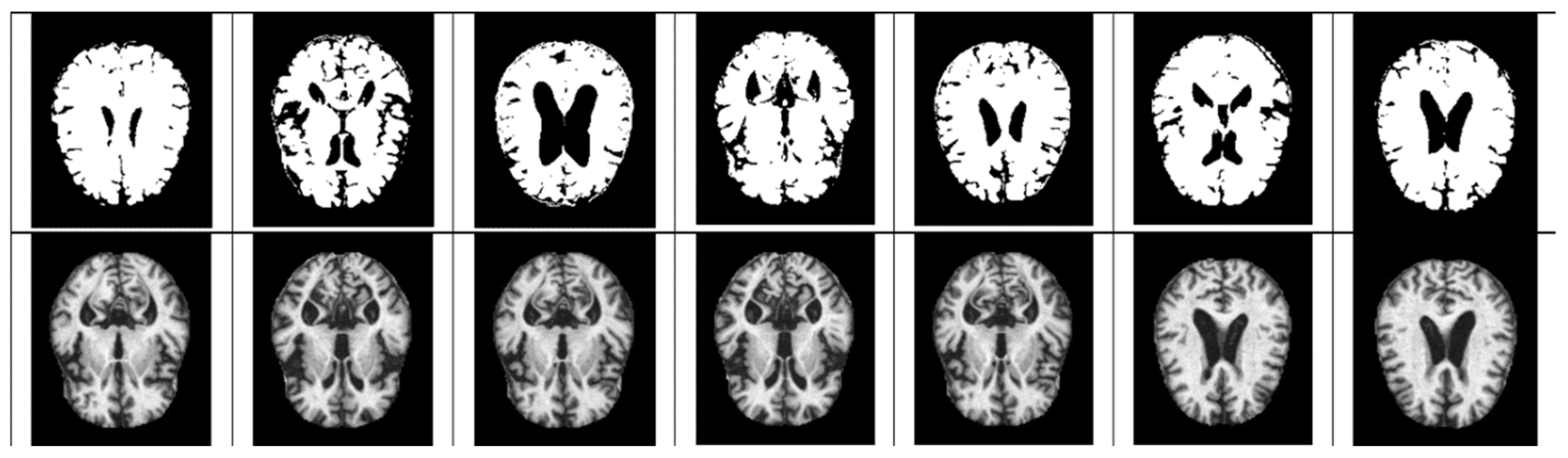
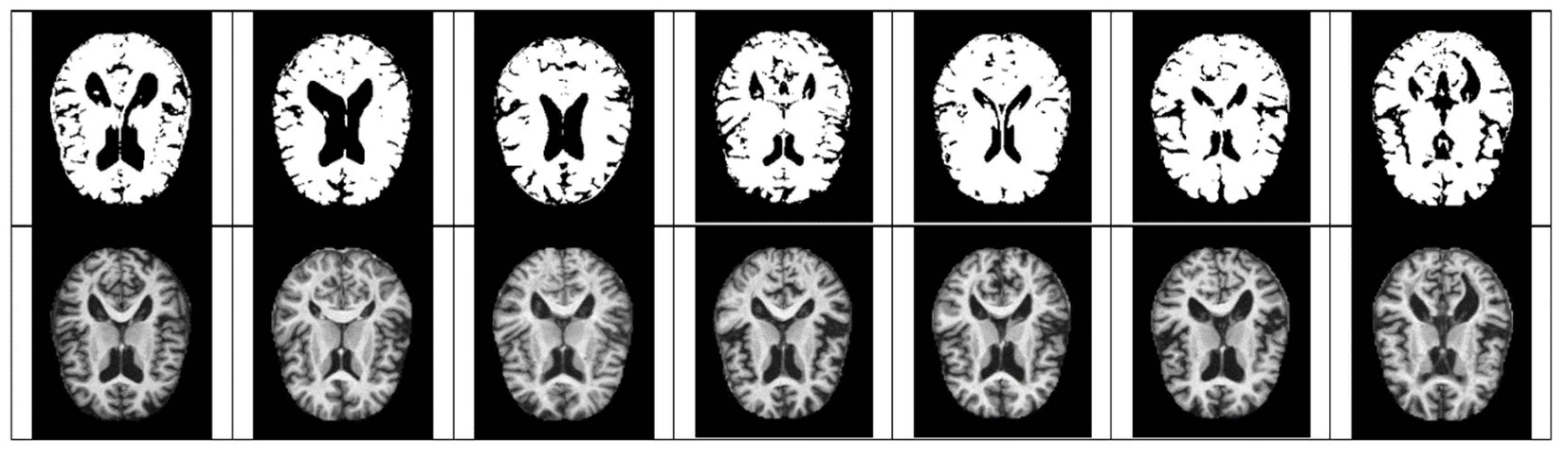
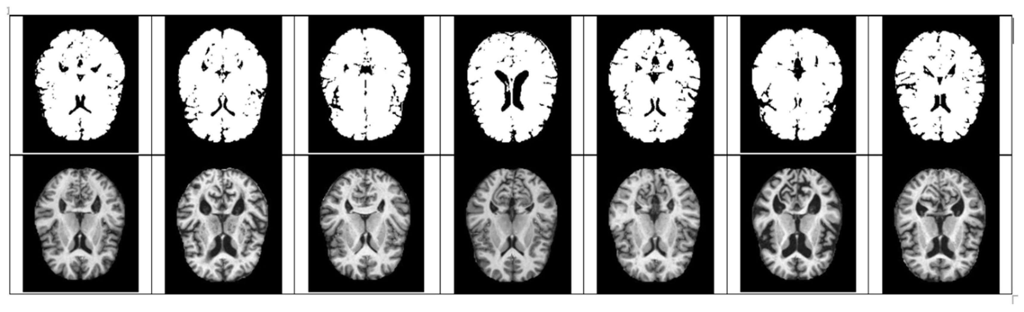
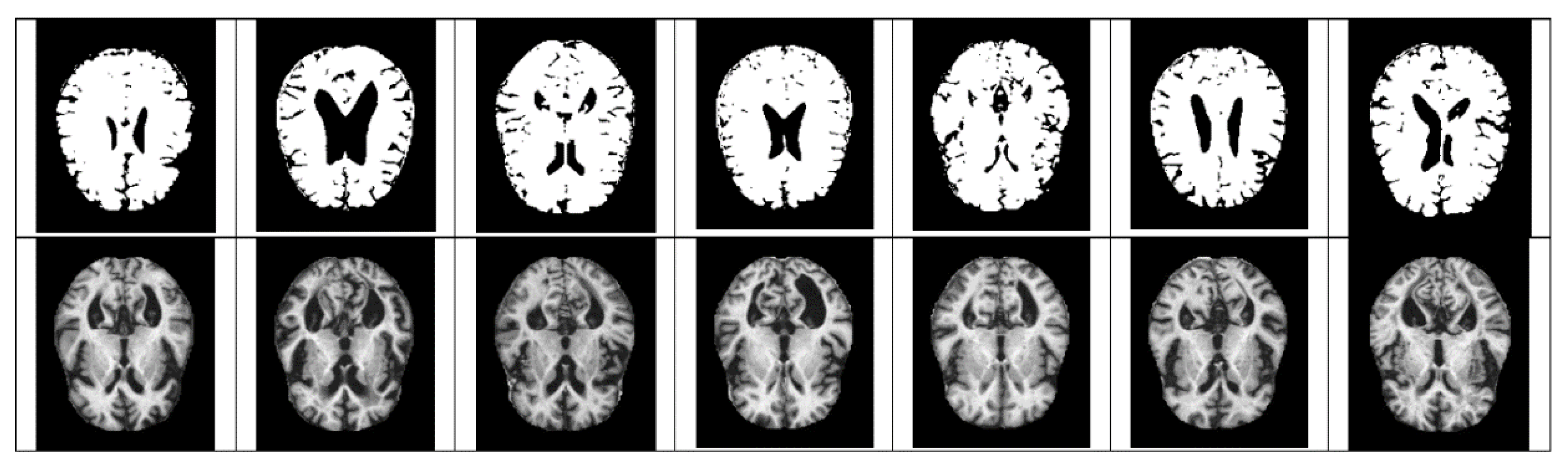
• The size space of pixels constituting the Alzheimer’s MRI data set is [0, 255]. Among them, patients with AD with reduced hippocampus will have more pixels close to zero than normal people. On the premise of this, the average value of pixel intensities in each MRI image is set as a threshold value. Alzheimer’s should recognize changes in size contraction rather than changes in brain function. Based on this information, it is necessary to set the space as an important feature for the color information of MRI rather than a feature representing the shape of the brain.
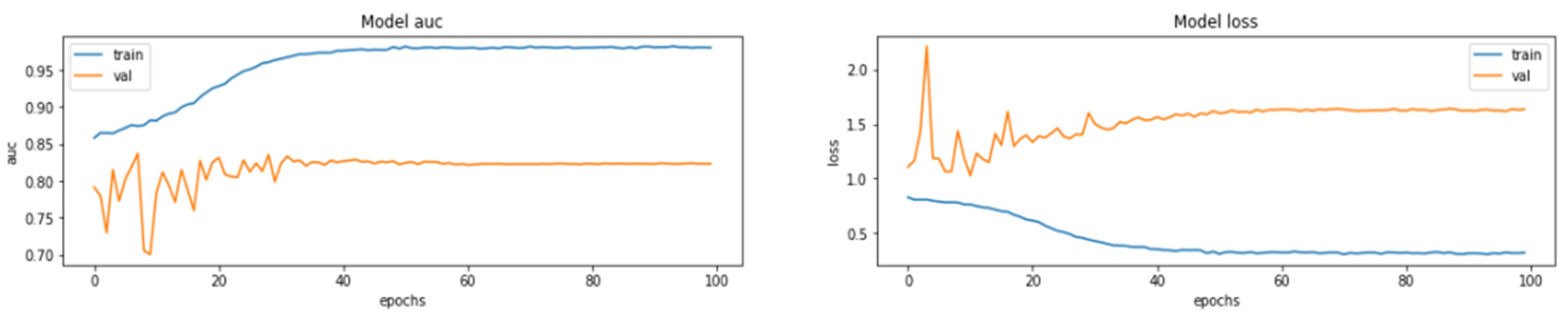
• Among the VGG family, the VGG-C Transform model with batch normalization added to the VGG-C model showed the highest performance with a test accuracy of about 0.9999. However, since the size of the MRI image is 208 × 176, distortion and loss of pixel information occur in the process of resizing to 224 × 224. Therefore, we propose a VGG model-based architecture that can learn while maintaining the original MRI size. Existing CNNs report high performance for images with the same aspect ratio. This is because images in the real world vary in size and need to be transformed into fixed-size metrics to learn through CNN. However, since all images in a given data set have the same aspect ratio, it is important to find input values of appropriate size. Moreover, due to the data imbalance problem, the AUC score is used as an evaluation indicator. The rest of the paper is arranged as follows: Section 2 describes the related studies. The proposed method is explained in Section 3. Section 4 summarizes the results. The discussion is presented in Section 5, and the conclusion is given in Section 6.

2. Related Work

It is believed that deep learning focuses on its use in the diagnosis of AD. Several in-depth study methods have recently been proposed to help diagnose AD and help physicians make informed health decisions. In this section, we present some studies that are closely related to our study. Lu nar. [12] proposed a multimodal deep neural network with a multi-step technique for identifying people with mental disabilities. The method has an accuracy of 82.4% in patients with mild cognitive impairment (MCI) and AD within three years. The model has a sensitivity of 94.23% in the AD category and an accuracy of 86.3% in the non-dementia category. Using ADNI and the National Center for Dementia Research (NRCD) data sets, Gupta nar. [13] proposed a diagnostic method for classifying ADs using cortical, subcortical, and hippocampal region features from MRI images with an accuracy of 96.42%. AD and healthy control (HC). Ahmed et al. [14] proposed a CNN model of a character extractor and a SoftMax classifier to diagnose AD. This model uses the right and left hippocampal sections on MRI to prevent overload and has an accuracy of 90.05%. Bashar nar. [15] developed a method of localization of the target region from a large MRI scale to automate the process. Based on the left and right hippocampus, this method achieves 94.82% and 94.02% accuracy, respectively.

Navaz nar. [16] proposed a pre-prepared Alexnet model to classify the stages of AD to solve the class imbalance model. The prefabricated model is used as a feature sorting device and is classified with the highest accuracy of 99.21% using support vector machine (SVM), k-nearest neighbor (KNN) and random forest (RF). Ieracitano et al. [17] proposed a data-based approach to differentiate subjects with AD, MCI, and HC by analyzing non-invasive EEG recordings. The energy spectral densities of the 19-channel EEG traces reflect their corresponding spectral profiles on a two-dimensional gray image. The CNN model is then used to classify binary classes and multi-categories from 2D images with 89.8% and 83.3% accuracy. Jain sun. [18] used the pre-prepared VGG16 model for feature unpacking, which uses “FreeSurfer” library for pre-processing, selection of MRI slices using entropy, and classification using a transfer training called PFSECTL mathematical model. Using the ADNI database, the researchers classified normal control (NC), early mci (EMCI), and late mci (LMCI) with a 95.73% accuracy. Mehmood sun. [19] used tissue segmentation to extract gray matter (GM) from each subject. This model achieves a classification accuracy of 98.73% for AD and NC and 83.72% for EMCI and LMCI patients. Shi et al. [20] proposed a deep multi-member network that works well for small and large data sets to diagnose AD. The model uses an ADNI data set with an accuracy of 55.34% in both binary and multi-class. Liu et al. [21] proposed the Siamese neural network to study the ability to differentiate all brain volume inequalities.

The team used a unique nonlinear nuclear approach to normalize features and eliminate package effects in the data set and population, while using MRI Cloud processes to create low-dimensional volume characteristics in a predetermined atlas brain structure. Networks use the ADNI data set to achieve a balanced accuracy of 92.72% in the MCI and AD categories. Van et al. [22] introduced a 3D ensemble model integration with AD and MCI using a collapsible grid method. The 3D-DenseNets were optimized using a probability-based melting method. This model uses ADNI data sets to achieve 97.52% class accuracy. Shankar nar. [23] used the wolf solution optimization method with the decision tree, KNN, and CNN models to diagnose AD with an accuracy of 96.23%. Jangel and Rator [24] proposed a pre-prepared VGG16 to extract AD features from the ADNI database. In their classification, they used clusters and decision tree algorithms meaning SVM, Linear Discriminate, and K. Their method had a 99.95% accuracy of functional MRI images and an average of 73.46% accuracy of PET images. Ge et al. [25] proposed a 3D multidimensional in-depth learning architecture to learn the features of AD. On a randomly isolated brain scanned data set of the subject, the system achieved an experimental accuracy of 93.53% and an average accuracy of 87.24%. Wang [26] introduced the Spike Convolutional Deep Boltzmann Machine model for early detection of AD with a multi-task learning technique to prevent hybrid mapping and over-tuning. Sarraf et al. [27] introduced an in-depth training line trained with multiple training drawings to perform specific classifications on scale and transition invariant processes. The model achieved 94.32% and 97.88% for functional MRI and MRI imaging. Preferred sun. [28], using data extension system, solved the problem of class imbalance in the detection of AD, achieving a classification accuracy of 98.41% in one view of the OASIS data set and 95.11% in 3D imaging.

Table 1 provides an overview of the literature study, and accordingly, many techniques have been proposed for classifying AD using machines and in-depth learning methods. However, high design parameters and class imbalances in the multi-category AD category remain a problem. To solve this problem, we proposed a CNN model with few parameters. We used the SMOTE [29] technique to resolve data classification imbalances, and our proposed model can accurately identify and predict the four stages of dementia that may lead to AD.

Table 1. A summary of the literature survey.

Ref.	Method	Author’s Name	No. of. Classes	Accuracy (%)
[12]	Multiscale deep learning	Lu nar	Binary Class (AD vs. HC)	82.4
[13]	Combined feature technique	Gupta nar	Binary Class (AD vs. HC)	96.42
[14]	Ensemble model	Ahmed et al.	Binary Class (AD vs. HC)	94.03
[17]	2D CNN	Ieracitano et al.	Binary Class (AD, MCI)	89.8
[18]	CNN	Jain sun	Three class (NC, EMCI, LMCI)	95.73
[19]	Transfer Learning	Mehmood sun	Binary class (AD vs. NC)	98.73
[20]	Deep polynomial network	Shi et al.	Multiclass (AD vs. NC)	55.34
[21]	Siamese network	Liu et al.	Binary class (MCI vs. AD)	92.72
[22]	3D CNN	Van et al.	Binary class (AD vs. MCI)	97.52
[24]	VGG16	Jangel and Rator	Binary class (AD vs. NC)	73.46
[25]	3D CNN	Ge et al.	Binary class (AD vs. NC)	93.53
[28]	3D View model	Preferred sun	Binary class (AD vs. NC)	95.11

3. Materials and Method

Alzheimer’s disease can be diagnosed by magnetic resonance imaging (MRI) of the brain [10]. In general, AD is diagnosed when the size of the hippocampus shown on the cerebral cortex is smaller than that of a normal person. MRI data set provided the information about the size of each patient’s hippocampus. However, due to the shape of the human brain, the AD machine learning model requires a great deal of complexity. Given a set of data, there is a major problem of information imbalance. As shown in Figure 1, of Kaggle, MildDementia has 717 units, Moderate Dementia has 52 units, NonDementia has 2560 units, and VeryMild Dementia has 1792 units.

Figure 1. Categories of dementia level in dataset.

3.1. Data Preprocess

As mentioned above, the method of diagnosing AD on MRI images [30] is to compare the size of the hippocampus. However, due to the characteristics of the existing CNN model, it is difficult to detect it because it is not sensitive to the variance of the image. Therefore, additional processing for the color space of the image is required. Moreover, this is a grayscale image, but it is stored as a 3D RGB value, so it needs to be converted to 2D. Therefore, additional processing for the color space of the image is required. To this end, the following activities have been proposed and implemented, as shown in Figure 2.

Figure 2. VGG-C Transform model process by MRI data.

In the case of Z-score standardization, the section to which each pixel belongs is converted to [−1, 1], and in the case of min–max, it is converted to [0, 1]. The pixel intensity of [0, 255] is scaled for fast convergence and accurate feature extraction during the computation of the convolutional neural network. Pixels constituting the Alzheimer’s MRI dataset have a size space of [0, 255]. Among them, Alzheimer’s patients with reduced hippocampus will have more pixels close to zero as compared to those of the normal people. Based on this premise, the average value of pixel intensity in each MRI image is set as the threshold. Alzheimer’s should recognize changes in size contraction rather than changes in brain features. Based on this information, it is necessary to set the empty space as an important feature for the color information of the MRI rather than the feature representing the shape of the brain. Therefore, Figure 3, Figure 4, Figure 5 and Figure 6 show examples of brain structure dataset changed to the Quantization Pixel intensity methodology.

Figure 3. Quantized very mild examples (above), original very mild examples (below).

Figure 4. Quantized non examples (above), original very mild examples (below).

Figure 5. Quantized moderate examples (above), original very mild examples (below).

Figure 6. Quantized mild examples (above), original very mild examples (below).

3.1.1. Scaling

Z-score is a variation of scaling that represents the number of standard deviations away from the mean. z-score is usually used to ensure that the feature distributions have mean = 0 and std = 1. It is useful when there are a few outliers, but not so extreme that you need clipping. One of the major sources of confusion between scaling and normalization is when the terms are sometimes used interchangeably and very similar. In both cases, it is necessary to transform the values of numeric variables so that the transformed data points have specific helpful properties. The difference is that, in scaling, you are changing the range of your data, while in normalization, you are changing the shape of the distribution of data. In the case of Z-score standardization, the section to which each pixel belongs is converted to [−1, 1], and in the case of Min–Max normalization, it is converted to [0, 1]. The pixel intensity of [0, 255] is scaled for fast convergence and accurate feature extraction during the computation of the convolutional neural network.

Scaling A. Z-score

$$\mathrm{Z}-score=\frac{data-mean\left(data\right)}{std\left(data\right)}$$

(1)

$$Min Max=\frac{data-min\left(data\right)}{ max\left(data\right)-min\left(data\right)}$$

(2)

3.1.2. Quantize Pixel Intensity

Pixels constituting the Alzheimer’s MRI dataset have a size space of [0, 255]. Among them, Alzheimer’s patients with reduced hippocampus will have more pixels close to zero than normal people. Based on this premise, the average value of pixel intensity in each MRI image is set as the threshold.

$$\begin{gathered} Quentized data=if data\left[i\right] \ge threshold, then data\left[i\right] ≔ 255 \\ else data\left[i\right] ≔ 0 \end{gathered}$$

(3)

The metrics used to analyze the study’s outputs included precision, recall, F-Score, and accuracy. These metric values were computed using the confusion matrix. These metrics’ equations are:

$$Accuracy (\%)=\left(TP+TN\right)/\left(TP FP TN FN\right)$$

(4)

$$Precision \left(PPV\right)=TP/\left(TP FP\right)$$

(5)

$$Recall=TP/\left(TP+FN\right)$$

(6)

$$F-score=2\left(Percision \ast Recall\right) Percion+Recall$$

(7)

3.1.3. ConvNet Configuration

The deep learning model used in the experiment was conducted based on the six models implemented in the VGG model paper, and the model structure is shown in Table 2 below. The convolutional layers in VGG use a very small receptive field (3 × 3, the smallest possible size that still captures left/right and up/down). There are also 1 × 1 convolution filters that act as linear transformation of the input, followed by a ReLU [31] unit. The convolution stride is fixed to 1 pixel so that the spatial resolution is preserved after convolution. Table 2 shows the ConvNet configurations evaluated in this study, one per column. Moving forward, we will refer to nets by name (A–E). All configurations follow the general design presented in the Section 3.1.3, differing only in depth: from 11 weighting layers in network A (8 transitions and 3 FC layers) to 19 weighting layers in network E (16 transitions and 3 FC layers). Transition of width layers (number of channels) start at 64 in the first layer and increase by doubling after each max pooling layer until 512. Table 2 shows the number of parameters for each configuration. Despite the great depth, the number of weights in the net is not greater than the number of weights in shallow nets with larger transitions. Layer width and receptive field (144M weights (Sermanet et al., 2014)).

Table 2. Model Structure.

ConvNet Configuration
A	A-LRN	B	C	D	E
11 weight layers	11 weight layers	13 weight layers	16 weight layers	16 weight layers	19 weight layers
Input (224 × 224 RGB image)
Conv3-64	Conv3-64 LRN	Conv3-64 Conv3-64	Conv3-64 Conv3-64	Conv3-64 Conv3-64	Conv3-64 Conv3-64
Maxpool
Conv3-128	Conv3-128	Conv3-128 Conv3-128	Conv3-128 Conv3-128	Conv3-128 Conv3-128	Conv3-128 Conv3-128
Maxpool
Conv3-256 Conv3-256	Conv3-256 Conv3-256	Conv3-256 Conv3-256	Conv3-256 Conv3-256 Conv1-256	Conv3-256 Conv3-256 Conv3-256	Conv3-256 Conv3-256 Conv3-256 Conv3-256
Maxpool
Conv3-512 Conv3-512	Conv3-512 Conv3-512	Conv3-512 Conv3-512	Conv3-512 Conv3-512 Conv1-512	Conv3-512 Conv3-512 Conv3-512	Conv3-512 Conv3-512 Conv3-512 Conv3-512
Maxpool
Conv3-512 Conv3-512	Conv3-512 Conv3-512	Conv3-512 Conv3-512	Conv3-512 Conv3-512 Conv1-512	Conv3-512 Conv3-512 Conv3-512	Conv3-512 Conv3-512 Conv3-512 Conv3-512
Maxpool
FC-4096
FC-4096
FC-1000
Soft-max

4. Experiment and Results

We performed 5-way cross-validation for all models, and the accuracy of the VGG-C with Tuning model that added the batch normalization process to the VGG-C model was 0.9800, and 0.9927, and 0.9906 for F1-score, precision, and recall, respectively, and 0.9947. Table 3 below shows the learning results. As shown in Figure A1, we made our VGG-C Transform model using Google Colab.

Table 3. Comparison of the result with other methods.

Model		VGG A	VGG B	VGG-C T	VGG D	VGG E	Our Work
Train	Accuracy	0.9876	0.8990	0.9800	0.9663	0.9143	0.9999
	F1-score	0.9945	0.9185	0.9927	0.9837	0.9284	0.9998
	Precision	0.9945	0.9173	0.9906	0.9941	0.9706	0.9997
	Recall	0.9945	0.9197	0.9947	0.9735	0.8897	1.0000
Test	Accuracy	0.7550	0.7480	0.8013	0.7415	0.7245	0.7746
	F1-score	0.7696	0.7513	0.8040	0.7380	0.7097	0.7799
	Precision	0.7702	0.7372	0.7895	0.7761	0.7553	0.7744
	Recall	0.7697	0.7659	0.8191	0.7035	0.6693	0.7855

4.1. Software Tools for Experimental

We implemented our proposal by experimenting using Python in Google Colaboratory with Tensorflow 2.0 and Keras 2.4.3; during training, we used a Tesla T4 GPU with 16 GB of memory provided by Colab.

4.2. Quantize Pixel Intensity

Alzheimer’s disease a should recognize changes in size contraction rather than changes in brain features. Based on this information, it is necessary to set the empty space as an important feature for the color information of the MRI rather than the feature representing the shape of the brain. Figure 3, Figure 4, Figure 5 and Figure 6 show examples of brain structure dataset changed to the Quantization Pixel intensity methodology.

4.3. Design Experiments

The performance of the proposed MLR-VGGNet was proven by a comparison on various CNN models, such as the original VGG16, VGG19, ResNet50, Inception V3, and Xception. In all comparison models, a transfer learning from pre-trained weights available was also used. The training parameters on all models is given, such as batch size = 20, epoch = 60, optimizer = RMSProp, learning rate = 1 × 10⁻⁵, loss function = categorical cross-entropy.

During training, the four blocks of VGGNet were frozen; therefore, the weights did not change to retain the lower layers generalized to generate low-level features. Additional components, such as AC, BN, and residuals, are fully trained to achieve weight with high-level feature generation that corresponds to the fish species classification.

4.4. Experimental Results

Among the VGG Family, the VGG-C Transform model with batch normalization [32] added to the VGG-C model recorded the highest performance with a test accuracy of approximately 0.9800. However, since the MRI image has a size of 208 × 176, distortion and loss of pixel information occur in the process of resizing it to 224 × 224. Our proposed VGG model-based architecture can learn while preserving the original MRI size [33]. Conventional CNNs report high performance for images with the same aspect ratio. This is because images have different sizes, so they need to be converted into metrics of a fixed size in order to learn them through CNN [7]. However, since all images in a given dataset have the same aspect ratio, it is important to find an input value of an appropriate size. In addition, due to data imbalance, the AUC Score should be used as an evaluation index. The Convolution2D layer in TensorFlow is designed to be suitable for convolution of feature maps with similar aspect ratios. Therefore, not a general Convolution2D layer, but a SeparableConvolution2D layer is required. The model is implemented so that learning can proceed through MLP through flattening after convolution operation [34].

The input size of the constructed model is 176 × 208 × 3, and all RGB values for each channel are data composed by repeating the gray scale of the two-dimensional matrix. From this image, a feature map is extracted through one block, consisting of a convolutional layer and a max pooling layer, and a new feature is extracted by passing the extracted feature map through a second convolutional block. The finally generated feature map is then flattened and passed through the MLP layer to predict the result. In the model compilation process, the optimizer used Adam and the learning rate schedule was applied. The loss function uses categorical cross entropy because it should be possible to predict four classes. Accuracy uses the AUC score due to the problem of class imbalance. The graph below is the result of learning by setting the model epoch to 100. The left graph shows the AUC score, and the right graph shows the loss. As shown in Figure 7, Figure 8 and Figure 9.

Figure 7. Accuracy graph.

Figure 8. Loss graph.

Figure 9. The AUC score for the train set was measured to be 0.9804, and the AUC score for the test set was measured to be 0.8232.

5. Discussion

In this paper, we proposed an enhanced prediction method for Alzheimer’s disease using quantize method to MRI Dataset conversion with the convolutional neural network (CNN) consisting of a VGG-C Transform model and a batch normalization. Four types of MRI Dataset are used by many pieces of research for predicting AD (Alzheimer’s Disease) but there is a problem with the imbalance between the class. The number of files was 4600 in the train dataset and 1279 in the test dataset, and the number of each class shows a difference of up to 300:1 for the train set. This imbalance not only greatly affects the performance of the model but also means a model of low judgment that cannot be judged on a small number of datasets. To solve this imbalance, we apply image quantizing method to simplify and maximize the feature, which is important to recognize changes in size contraction rather than changes in brain features. After the experiment, the AUC score improved by up to 1.19%, compared to the normal dataset, and it can be seen as a meaningful result because medical images, such as MRI data, are important in the judgment of clinicians. A limitation of our work is the lack of MRI datasets from real patients, so in future work, we are trying to find clinicians who can collaborate on clinical trial studies with Institutional Review Board (IRB) approval.

6. Conclusions

In this paper, we propose an improved prediction method for Alzheimer’s disease using a quantization method that transforms the MRI data set using a VGG-C Transform model and a convolutional neural network (CNN) consisting of batch normalization. Among the VGG Family, the VGG-C Transform model with batch normalization added to the VGG-C model recorded the highest performance with a test accuracy of about 0.9999. However, since the MRI image has a size of 208 × 176, distortion and loss of pixel information occur in the process of resizing it to 224 × 224. Therefore, we proposed a VGG model-based architecture that can learn while preserving the original MRI size. As a result, we were able to obtain a prediction accuracy of 98%, and the AUC score increased by up to 1.19%, compared to the normal MRI image data set. It is expected that our study will be helpful in predicting Alzheimer’s disease using the MRI dataset. Furthermore, if the data used are adequate and the available resources can handle the increased computational complexity, the overall performance of the base model to be enhanced by fine-tuning the pre-trained convolutional layers.

References

- Liu, S.; Liu, S.; Cai, W.; Che, H.; Pujol, S.; Kikinis, R.; Feng, D.; Fulham, M.J. Multimodal neuroimaging feature learning for multiclass diagnosis of Alzheimer’s disease. IEEE Trans. Biomed. Eng. 2015, 62, 1132–1140. [Google Scholar] [CrossRef] [PubMed]
- Przedborski, S.; Vila, M.; Jackson-Lewis, V. Series introduction: Neurodegeneration: What is it and where are we? J. Clin. Investig. 2003, 111, 3–10. [Google Scholar] [CrossRef] [PubMed]
- Giorgio, J.; Landau, S.M.; Jagust, W.J.; Tino, P.; Kourtzi, Z. Modelling prognostic trajectories of cognitive decline due to Alzheimer’s disease. NeuroImage Clin. 2020, 26, 102199. [Google Scholar] [CrossRef] [PubMed]
- Patterson, C. World Alzheimer Report 2018 the State of the Art of Dementia Research: New Frontiers; Alzheimer’s Disease International: London, UK, 2018. [Google Scholar]
- Alzheimer’s Disease Fact Sheet. 2019. Available online: https://www.nia.nih.gov/health/alzheimers-disease-fact-sheet (accessed on 11 May 2022).
- Stamate, D.; Smith, R.; Tsygancov, R.; Vorobev, R.; Langham, J.; Stahl, D.; Reeves, D. Applying deep learning to predicting dementia and mild cognitive impairment. In Artificial Intelligence Applications and Innovations (IFIP Advances in Information and Communication Technology); Springer: Cham, Switzerland, 2020; Volume 584, pp. 308–319. [Google Scholar] [CrossRef]
- De, A.; Chowdhury, A.S. DTI based Alzheimer’s disease classification with rank modulated fusion of CNNs and random forest. Expert Syst. Appl. 2021, 169, 114338. [Google Scholar] [CrossRef]
- Ieracitano, C.; Mammone, N.; Hussain, A.; Morabito, F.C. novel multi-modal machine learning based approach for automatic classification of EEG recordings in dementia. Neural Netw. 2020, 123, 176–190. [Google Scholar] [CrossRef]
- Kim, Y. Are we being exposed to radiation in the hospital? Environ. Health Toxicol. 2016, 31, e2016005. [Google Scholar] [CrossRef]
- KaggleDataset. Available online: https://www.kaggle.com/datasets/jboysen/mri-and-alzheimers (accessed on 19 May 2022).
- Moser, E.; Stadlbauer, A.; Windischberger, C.; Quick, H.H.; Ladd, M.E. Magnetic resonance imaging methodology. Eur. J. Nucl. Med. Mol. Imag. 2009, 36, 30–41. [Google Scholar] [CrossRef]
- Mansourifar, H.; Shi, W. Deep Synthetic Minority Oversampling Technique. arXiv 2020, arXiv:2003.09788. [Google Scholar]
- Dubey, S. Alzheimer’s Dataset. 2019. Available online: https://www.kaggle.com/tourist55/alzheimers-dataset-4-class-of-images (accessed on 19 May 2022).
- Rieke, J.; Eitel, F.; Weygandt, M.; Haynes, J.D.; Ritter, K. Visualizing convolutional networks for MRI-based diagnosis of Alzheimer’s disease. In Understanding and Interpreting Machine Learning in Medical Image Computing Applications (Lecture Notes in Computer Science); Springer: Cham, Switzerland, 2018; Volume 11038, pp. 24–31. [Google Scholar] [CrossRef]
- Lu, D.; Initiative, A.D.N.; Popuri, K.; Ding, G.W.; Balachandar, R.; Beg, M.F. Multimodal and multiscale deep neural networks for the early diagnosis of Alzheimer’s disease using structural MR and FDG-PET images. Sci. Rep. 2018, 8, 5697. [Google Scholar] [CrossRef]
- Gupta, Y.; Lee, K.H.; Choi, K.Y.; Lee, J.J.; Kim, B.C.; Kwon, G.R. Early diagnosis of Alzheimer’s disease using combined features from voxel-based morphometry and cortical, subcortical, and hippocampus regions of MRI T1 brain images. PLoS ONE 2019, 14, e0222446. [Google Scholar] [CrossRef]
- Ahmed, S.; Choi, K.Y.; Lee, J.J.; Kim, B.C.; Kwon, G.-R.; Lee, K.H.; Jung, H.Y. Ensembles of patch-based classifiers for diagnosis of alzheimer diseases. IEEE Access 2019, 7, 73373–73383. [Google Scholar] [CrossRef]
- Basher, A.; Kim, B.C.; Lee, K.H.; Jung, H.Y. Volumetric featurebased Alzheimer’s disease diagnosis from sMRI data using a convolutional neural network and a deep neural network. IEEE Access 2021, 9, 29870–29882. [Google Scholar] [CrossRef]
- Nawaz, H.; Maqsood, M.; Afzal, S.; Aadil, F.; Mehmood, I.; Rho, S. A deep feature-based real-time system for alzheimer disease stage detection. Multimed. Tools Appl. 2020, 80, 1–19. [Google Scholar] [CrossRef]
- Ieracitano, C.; Mammone, N.; Bramanti, A.; Hussain, A.; Morabito, F.C. A convolutional neural network approach for classification of dementia stages based on 2D-spectral representation of EEG recordings. Neurocomputing 2019, 323, 96–107. [Google Scholar] [CrossRef]
- Jain, R.; Jain, N.; Aggarwal, A.; Hemanth, D.J. Convolutional neural network based Alzheimer’s disease classification from magnetic resonance brain images. Cognit. Syst. Res. 2019, 57, 147–159. [Google Scholar] [CrossRef]
- Mehmood, A.; Yang, S.; Feng, Z.; Wang, M.; Ahmad, A.S.; Khan, R.; Maqsood, M.; Yaqub, M. A transfer learning approach for early diagnosis of Alzheimer’s disease on MRI images. Neuroscience 2021, 460, 43–52. [Google Scholar] [CrossRef]
- Shi, J.; Zheng, X.; Li, Y.; Zhang, Q.; Ying, S. Multimodal neuroimaging feature learning with multimodal stacked deep polynomial networks for diagnosis of Alzheimer’s disease. IEEE J. Biomed. Health Informat. 2018, 22, 173–183. [Google Scholar] [CrossRef]
- Liu, C.-F.; Padhy, S.; Ramachandran, S.; Wang, V.X.; Efimov, A.; Bernal, A.; Shi, L.; Vaillant, M.; Ratnanather, J.T.; Faria, A.V.; et al. Using deep siamese neural networks for detection of brain asymmetries associated with Alzheimer’s disease and mild cognitive impairment. Magn. Reson. Imag. 2019, 64, 190–199. [Google Scholar] [CrossRef]
- Wang, H.; Shen, Y.; Wang, S.; Xiao, T.; Deng, L.; Wang, X.; Zhao, X. Ensemble of 3D densely connected convolutional network for diagnosis of mild cognitive impairment and Alzheimer’s disease. Neurocomputing 2019, 333, 145–156. [Google Scholar] [CrossRef]
- Shankar, K.; Lakshmanaprabu, S.K.; Khanna, A.; Tanwar, S.; Rodrigues, J.J.; Roy, N.R. Alzheimer detection using group grey wolf optimization based features with convolutional classifier. Comput. Electr. Eng. 2019, 77, 230–243. [Google Scholar] [CrossRef]
- Janghel, R.; Rathore, Y. Deep convolution neural network based system for early diagnosis of Alzheimer’s disease. IRBM 2020, 1, 1–10. [Google Scholar] [CrossRef]
- Ge, C.; Qu, Q.; Gu, I.Y.-H.; Jakola, A.S. Multiscale deep convolutional networks for characterization and detection of Alzheimer’s disease using MR images. In Proceedings of the 2019 IEEE International Conference on Image Processing (ICIP), Taipei, Taiwan, 22–25 September 2019; Volume 12, pp. 789–793. [Google Scholar] [CrossRef]
- Pan, T.; Zhao, J.; Wu, W.; Yang, J. Learning imbalanced datasets based on SMOTE and Gaussian distribution. Inf. Sci. 2020, 512, 1214–1233. [Google Scholar] [CrossRef]
- Bi, X.; Wang, H. Early Alzheimer’s disease diagnosis based on EEG spectral images using deep learning. Neural Netw. 2019, 114, 119–135. [Google Scholar] [CrossRef] [PubMed]
- Brownlee, J. A Gentle Introduction to the Rectified Linear Unit (ReLU). 2020. Available online: https://machinelearningmastery.com/rectified-linear-activation-function-for-deep-learning-neural-networks/ (accessed on 21 May 2022).
- Sarraf, S.; DeSouza, D.D.; Anderson, J.; Tofighi, G. DeepAD: Alzheimer’s disease classification via deep convolutional neural networks using MRI and fMRI. bioRxiv 2016. [Google Scholar] [CrossRef]
- Afzal, S.; Maqsood, M.; Nazir, F.; Khan, U.; Aadil, F.; Awan, K.M.; Mehmood, I.; Song, O.-Y. A data augmentationbased framework to handle class imbalance problem for Alzheimer’s stage detection. IEEE Access 2019, 7, 115528–115539. [Google Scholar] [CrossRef]
- Jordan, J. Normalizing Your Data. 2018. Available online: https://www.jeremyjordan.me/batch-normalization/ (accessed on 21 May 2022).