UCAV Air Combat Maneuver Decisions Based on a Proximal Policy Optimization Algorithm with Situation Reward Shaping

Abstract

Autonomous maneuver decision by an unmanned combat air vehicle (UCAV) is a critical part of air combat that requires both flight safety and tactical maneuvering. In this paper, an unmanned combat air vehicle air combat maneuver decision method based on a proximal policy optimization algorithm (PPO) is proposed. Firstly, a motion model of the unmanned combat air vehicle and a situation assessment model of air combat was established to describe the motion situation of the unmanned combat air vehicle. An enemy maneuver policy based on a situation assessment with a greedy algorithm was also proposed for air combat confrontation, which aimed to verify the performance of the proximal policy optimization algorithm. Then, an action space based on a basic maneuver library and a state observation space of the proximal policy optimization algorithm were constructed, and a reward function with situation reward shaping was designed for accelerating the convergence rate. Finally, a simulation of air combat confrontation was carried out, which showed that the agent using the proximal policy optimization algorithm learned to combine a series of basic maneuvers, such as diving, climb and circling, into tactical maneuvers and eventually defeated the enemy. The winning rate of the proximal policy optimization algorithm reached 62%, and the corresponding losing rate was only 11%.

1. Introduction

As a critical part of modern war, air combat intensively embodies the trend that emerging technologies are widely applied in war. Autonomous decision by an unmanned combat air vehicle (UCAV) is one of the main research directions in air combat. In the 1960s, the National Aeronautics and Space Administration (NASA) began an experiment using artificial intelligence (AI) to replace human pilots in making air combat decisions [1,2]. In 2016, Psibernetix Inc., Air Force Research Laboratory and University of Cincinnati, disclosed an AI called ALPHA, which controls the flights of UCAVs in air combat missions [3]. In 2019, the Defense Advanced Research Project Agency (DARPA) kicked off the Air Combat Evolution program (ACE), which is aimed at developing trusted, scalable, human-level, AI-driven autonomy for air combat [4].

The main advantages of UCAV autonomous air combat are as follows: improving the combat level of the pilot by man–machine confrontation training; easing the operational pressure of the pilot with decision support in air combat; reducing training time, costs and casualties by autonomous air combat or human–machine collaborative combat.

The theory and technology regarding autonomous air combat maneuver decision have been evolving in recent years. Traditional research methods include game theory, expert system and optimization theory.

Differential game theory is a typical representative air combat maneuver decision method based on game theory. Differential game of pursuit and evasion was introduced by Isaacs [5]. Sufficient conditions of qualitative differential game, which assure the termination of a particular target of a pursuit–evasion problem, were derived by Leitmann [6]. A differential game theory-based maneuver algorithm following a hierarchical decision structure was developed in [7]. The algorithm establishes a scoring function matrix computed from the relative geometry, relative distance and velocity of two aircrafts, and then it performs a scoring function matrix calculation based on differential game theory to determine the optimal maneuvers in a dynamic and challenging combat situation. The combat results and maneuvers under the controlled computation environment are similar to those of real air combat.

A rule-based expert system, which needs less effort to engineer and possesses high interpretability, constructs production rules with predicate logic similar to IF–ELSE–THEN. An air combat decision expert system was established in [8]. The system matches collected air combat situation information with the rules in an expert knowledge base, and then it outputs corresponding strategies. A systematic decision method based on an expert system was proposed in [9]. The method designs a maneuver selection auxiliary system, which is composed of a knowledge base, tactical planner, maneuver method selector, execution planner, special case processor and man–machine interface. The knowledge base is constructed according to expert evaluation of air combat decision. The other parts of the system are mainly constructed by fuzzy logic. This method can assist pilots in realizing the potential combat capability of the aircraft and meet the operational performance requirements within time limits. In [10], a rule base was established according to potential air combat situations faced by UCAVs, and the constraints of air combat decision were set with a priori knowledge. In [11], an evolutionary expert system tree method was proposed to solve the problem that traditional expert systems are unable to be applied in unexpected situations.

An air combat decision method based on an optimization algorithm formalizes decision-making problems into multiobjective optimization problems. In [12], a Bayesian inference-theory-based air combat situation assessment was calculated to adjust the weights of the maneuver decision factors. Functions based on fuzzy logic of the maneuver decision factors were established to enhance the robustness and effectiveness of the decision results. The simulation results demonstrated the intensity of the air combat game and displayed the drawbacks of an element maneuver method. An intelligent tactical aid decision system based on linear discriminant analysis (LDA) and improved glowworm swarm optimization (IGSO) was proposed in [13]. The simulation results showed that the LDA-IGSO-ELM algorithm can quickly and accurately solve the problem of threat assessment and provide effective support for firepower allocation and maneuver decision. The biological immune system protects the body against intruders by recognizing and destroying harmful cells or molecules. Inspired by this, [14] employed the genetic algorithm and evolutionary algorithm to imitate the immune mechanism to select and construct air combat maneuvers. The test results demonstrated the potential of immunized maneuver selection in terms of constructing effective motion-based trajectories over a relatively short (1–2 s) period of time. Reference [15] modeled air combat based on optimal control and game theory and then transformed dual aircraft air combat into an optimization problem using parameterized curves. The problem was then solved with a moving time horizon scheme to generate optimal strategies for the aircraft. The results from different scenarios showed that the method is capable of providing solutions in air combat for autonomous aerial vehicles.

Traditional air combat decision methods require accurate modeling of a complex and changeable air combat process, which is usually difficult to achieve. With the expansion of the decision space, it is also faced with dimension explosion, which leads to difficulties in solving problems and low real-time performance. Emerging research methods represented by deep reinforcement learning (DRL) train an agent through a trial-and-error mechanism, which removes accurate modeling and generates maneuver decision with data based on a neural network to improve solution efficiency [16].

The feasibility of autonomous maneuver decision based on reinforcement learning (RL) was proved in [17]. However, motion of UCAVs was only considered in the 2D plane, and research on the motion of UCAVs in the 3D space was lacking in the paper. An intelligent tactical decision method based on a deep Q-learning network (DQN) was proposed in [18]. In order to verify the validity of the method, an enemy based on Min-Max algorithm was also designed. The simulation results showed that the decision-making performance of the DQN approach was quicker and more effective than the Min-Max recursive approach. However, velocity was not considered as a feature vector in the input of the neural network, which may have affected the convergence rate of the method. In [19], a heuristic Q-network method was proposed to improve the efficiency of reinforcement learning, which realizes self-learning of air confrontation maneuver strategy and, finally, helps the fighters make reasonable maneuver decisions independently under different air confrontation situations. However, similar to [17], the influence of changes in altitude on the motion of UCAVs was not considered. In [20], an autonomous maneuver decision model based on a deep Q network was proposed for UCAVs in short-range air combat; however, velocity and angles were coupled in the definition of an air combat situational advantage, which may interfere in the process of learning optimal strategies with a reward function. A novel maneuver strategy generation algorithm based on a state-adversarial deep deterministic policy gradient algorithm was proposed in [21], but the experimental results in the paper only proved the effectiveness of the algorithm in the 2D plane.

There are two main inadequacies in the existing research on air combat maneuver decision based on deep reinforcement learning: one is that the training environment of the agent is different from actual air combat, which limits the application of the research results; the other is that factors affecting air combat are not fully considered, which affects the learning efficiency of the agent. In this paper, a novel UCAV air combat maneuver decision method based on a proximal policy optimization algorithm (PPO) [22] is proposed. Firstly, a general UAV short-range air combat confrontation framework was established including a motion model of a fixed-wing aircraft and a situation assessment model of air combat. In order to verify the effectiveness of the method, an enemy maneuver strategy based on a greedy algorithm was designed. Then, the action space based on a basic maneuver library and the state observation space of the agent were constructed. The maneuver policy was generated by training with the PPO algorithm. A reward function, based on situation reward shaping, was designed for accelerating the convergence rate of the algorithm. Finally, simulations of one-to-one, short-range air combat in stochastic situations were carried out to verify the effectiveness of the PPO algorithm. The winning rate of the PPO algorithm reached 62%, and the corresponding losing rate was only 11%. The results of the simulations showed that the maneuver decision method proposed in this paper can enable UCAVs to learn the maneuver policy autonomously and defeat the enemy.

The paper is arranged as follows: the general UCAV short-range air combat confrontation framework is constructed in Section 2; the agent training method based on deep reinforcement learning is designed in Section 3; the simulation analysis is performed in Section 4; Section 5 summarizes the research.

2. Air Combat Confrontation Framework

In this section, the simulation environment of general UCAV short-range air combat is constructed, which mainly included a UCAV motion model, air combat situation assessment model, and enemy maneuver strategy based on the situation assessment. The UCAV motion model provides a research object for air combat maneuver decision. The air combat situation assessment model is the basis for evaluating the advantages and disadvantages of the air combat maneuver decision, and the enemy maneuver strategy based on the situation assessment adds antagonism to the air combat simulation environment and serves as a training opponent to verify the effectiveness of the air combat maneuver decision based on deep reinforcement learning.

2.1. Unmanned Combat Air Vehicle Motion Model

The velocities and positions of UCAVs are the main factors that affect short-range air combat. Therefore, a three degrees of freedom model for a fixed-wing aircraft was employed in this paper, which not only reflected the air combat situation but also improved the simulation’s efficiency. Considering that the angle of attack and the angle of sideslip are so small that the two angles can be ignored, a dynamic model of a UCAV in the NED (north-east-down) coordinate system can be expressed as [23]:

$$\left\{\begin{array}{l}\dot{x}=v\cos \gamma \cos \psi \\ \dot{y}=v\cos \gamma \sin \psi \\ \dot{z}=-v\sin \gamma \\ \dot{v}=g\left(n_x-\sin \gamma \right)\\ \dot{\gamma }=\frac{g}{v}\left(n_z\cos \varphi -\cos \gamma \right)\\ \dot{\psi }=\frac{g\sin \varphi }{v\cos \gamma }{n}_z\end{array}\right.,$$

(1)

where $\mathit{p}=\left[x,y,z\right]$ represents the position, and the flight altitude of the UCAV is $h=-z$. $\dot{x}$, $\dot{y}$ and $\dot{z}$ denote the north velocity, the east velocity and the vertical velocity, respectively; $v$ represents the airspeed; $\gamma$ and $\psi$ denote the angle of climb and the azimuth angle of the flight path; respectively. The state variable $\mathit{s}$ is:

$$\mathit{s}=\left[x,y,z,v,\gamma ,\psi ,\dot{x},\dot{y},\dot{z},\dot{v},\dot{\gamma },\dot{\psi }\right].$$

(2)

where $\mathit{u}=\left[n_x,n_z,\varphi \right]$ is the control input of a UCAV; $n_x$ is the longitudinal overload, and its direction is consistent with the direction of the velocity vector; $n_z$ is the normal overload, and its direction is consistent with the direction of the lift; $\varphi$ is the roll angle with the velocity vector as the axis, and its definition conforms to the right-hand rule. The velocity magnitude can be changed by $n_x$, and the velocity direction can be changed by $n_z$ and $\varphi$. Therefore, the desired maneuvers of a UCAV can be achieved with an appropriate $\mathit{u}$ in theory. Considering the real conditions of the short-range air combat environment and the limited maneuverability of a UCAV, several limitations were set, $\left[x,y\right]\in \left[-2\times 10^4,2\times 10^4\right]$ m and $z\in \left[-2\times 10^4,-1\times {10}^2\right]$ m; $v\in \left[100,600\right]$ m/s; $n_x\in \left[-5,5\right]$ and $n_z\in \left[-5,5\right]$. The parameters of the UCAV motion model are shown in Figure 1.

2.2. Air Combat Situation Assessment Model

An air combat situation can be understood as qualitative or quantitative descriptions of various indicators of UCAVs including the position, velocity, firepower and relative position and velocity difference between UCAVs. The air combat situation is dynamic so that the descriptions in different evaluation systems may be different.

The geometry between two UCAVs can be determined by the relative angle and distance in the short-range air combat. The geometry of air combat is shown in Figure 2. The red aircraft represents the UCAV trained by deep reinforcement learning, and the blue aircraft represents the enemy UCAV. $\mathit{L}\mathit{O}\mathit{S}$ is line of sight, which is defined as the vector from the center of mass of the red UCAV to that of the blue UCAV, and its magnitude is the distance between the two UCAVs. $ATA$ is the antenna train angle, which is defined as the angle between the velocity vector of the red UCAV and the $\mathit{L}\mathit{O}\mathit{S}$, $ATA\in \left[0,\pi \right]$. $AA$ is the aspect angle, which is defined as the angle between the velocity vector of the blue UCAV and the $\mathit{L}\mathit{O}\mathit{S}$, $AA\in \left[0,\pi \right]$. $HCA$ is the heading crossing angle, which is defined as the angle between the velocity vectors of the two UCAVs, $HCA\in \left[0,\pi \right]$. The three-ninths line is the line between the 3 and 9 o’clock directions of an aircraft, which is used to determine whether the other aircraft is located in the front or rear hemisphere of the aircraft.

Let ${\mathit{p}}_r=\left[x_r,y_r,z_r\right]$ and ${\mathit{v}}_r=\left[v_r^x,v_r^y,v_r^z\right]$ denote the position and the velocity vector of the red UCAV, respectively, and ${\mathit{p}}_b=\left[x_b,y_b,z_b\right]$ and ${\mathit{v}}_b=\left[v_b^x,v_b^y,v_b^z\right]$ denote the position and the velocity vector of the blue UCAV, respectively. Then, the formula using the above parameters is as follows:

$$\mathit{L}\mathit{O}\mathit{S}={\mathit{p}}_b-{\mathit{p}}_r,$$

(3)

$$ATA=\arccos \left(\frac{{\mathit{v}}_r\cdot \mathit{L}\mathit{O}\mathit{S}}{‖{\mathit{v}}_r‖\cdot ‖\mathit{L}\mathit{O}\mathit{S}‖}\right),$$

(4)

$$AA=\arccos \left(\frac{{\mathit{v}}_b\cdot \mathit{L}\mathit{O}\mathit{S}}{‖{\mathit{v}}_b‖\cdot ‖\mathit{L}\mathit{O}\mathit{S}‖}\right),$$

(5)

$$HCA=\arccos \left(\frac{{\mathit{v}}_r\cdot {\mathit{v}}_b}{‖{\mathit{v}}_r‖\cdot ‖{\mathit{v}}_b‖}\right).$$

(6)

The situation assessment was divided into two parts: one was the conditions for the end of air combat including the attack zone, altitude limit and velocity limit; the other part was the situation assessment in the process of air combat including the angle, velocity and altitude situations.

2.2.1. Conditions for the End of Air Combat

Short-range air combat, also known as a dogfight, usually covers an operational range of 10 km, and the aim is to shoot down enemy aircraft or make them lose their combat capability. Therefore, whether the air combat is over can be judged by the following conditions:

• Shooting down the enemy or being shot down;
• Stalling or crashing.

The attack zone of a UCAV is limited due to the impact of the types and performances of weapons. In this paper, the attack zone was simplified to ${\mathbf{Z}}_{\alpha }$, which is the zone surrounded by red lines in Figure 3. $\alpha$ denotes the maximum attack angle of a UCAV, $\alpha \ge 0$. $R_{\min }$ denotes the minimum attack range, and $R_{\max }$ denotes the maximum attack range. If $ATA<\alpha$ and the distance of two UCAVs is greater than $R_{\min }$ and less than $R_{\max }$, the blue UCAV is in the attack zone of the red UCAV, so that the red UCAV will fire to shoot down the blue UCAV. On the contrary, the red UCAV will be shot down. The attack zone, ${\mathbf{Z}}_{\alpha }$, can be expressed as:

$${\mathbf{Z}}_{\alpha }=\left\{{\mathit{p}}_b\left|ATA\le \alpha ,R_{\min }\le ‖\mathit{L}\mathit{O}\mathit{S}‖\right.\le R_{\max }\right\}.$$

(7)

Aircraft with an extremely low velocity or altitude are not allowed in air combat. Therefore, the other condition for judging whether the air combat is over can be expressed as:

$$\left\{\begin{array}{l}\mathrm{end} \mathrm{of} \mathrm{air} \mathrm{combat},\\ \mathrm{air} \mathrm{combat} \mathrm{in} \mathrm{progress},\end{array}\right.\begin{array}{l}\hspace{1em}\mathrm{if}v\le v_{\min }\mathrm{or}h\le h_{\min },\\ \hspace{1em}\mathrm{else},\end{array}$$

(8)

where $v_{\min }$ and $h_{\min }$ denote the minimum allowable velocity and altitude of a UCAV, respectively.

In addition, it was necessary to limit the number of steps per episode in the simulation. Therefore, another condition for judging whether the air combat is over can be expressed as:

$$\left\{\begin{array}{l}\mathrm{end} \mathrm{of} \mathrm{air} \mathrm{combat},\\ \mathrm{air} \mathrm{combat} \mathrm{in} \mathrm{progress},\end{array}\right.\begin{array}{l}\hspace{1em}\mathrm{if}t\ge t_{\max },\\ \hspace{1em}\mathrm{else},\end{array}$$

(9)

where $t_{\max }$ denotes the maximum steps per episode.

2.2.2. Situation Assessment in the Process of Air Combat

This section takes the red UCAV as an example. In essence, the whole process of air combat can be understood as that the red UCAV avoids entering the attack zone of the blue UCAV and makes the blue UCAV enter that of the red UCAV by maneuvering. Figure 4 shows a top view of the attack zone. The red and the green parts represent the attack zone and the security zone, respectively.

According to Figure 2 and Figure 4, the smaller the $ATA$ and $AA$, the more favorable it is for the red UCAV in the same other conditions. In addition, flight safety is also a key factor affecting the situation according to Section 2.2.1. Therefore, the air combat situation, $\eta$, can be divided into four parts, which can be switched according to the state of the UCAV. The switching process is as follows (Algorithm 1).

Algorithm 1 Switching Process of an Air Combat Situation

If $v$ or $h$ are less than the threshold     $\eta ={\eta }_1\left(v,h\right)$    Else if $AA<90°$       $\eta ={\eta }_2\left(‖\mathit{L}\mathit{O}\mathit{S}‖\right)$       Else if distance is greater than the threshold

$\eta ={\eta }_3\left(AA\right)$          Else           $\eta ={\eta }_4\left(‖\mathit{L}\mathit{O}\mathit{S}‖\right)$

The first part of the situation model ${\eta }_1$ takes the velocity and altitude of the UCAV as variables. When the velocity or altitude is less than the threshold, ${\eta }_1$ takes effect, which is to ensure flight safety. The velocity index and altitude index of ${\eta }_1$ are as follows:

$${\eta }_v=-e^{-v/k_v},$$

(10)

$${\eta }_h=-e^{-h/k_h},$$

(11)

${\eta }_1$ is defined as:

$${\eta }_1={\eta }_v+{\eta }_h-2,$$

(12)

where $k_v$ and $k_h$ are constants used to adjust the trend of the index curves, ${\eta }_1\in \left[-4,-2\right)$, and ${\eta }_v$ and ${\eta }_h$ are shown in Figure 5.

The second part of the situation model, ${\eta }_2$, takes the distance between UCAVs as a variable. When the UCAV flies at a normal velocity and altitude, $AA\le \frac{\pi }{2}$, and ${\eta }_2$ takes effect, which aims to guide the UCAV to quickly approach the enemy and reach attack conditions. ${\eta }_2$ is defined as:

$${\eta }_2=0.5\left(e^{-‖\mathit{L}\mathit{O}\mathit{S}‖/k_d}-1\right),$$

(13)

where $k_d$ is a constant used to adjust the trend of ${\eta }_2$, ${\eta }_2\in \left(-0.5,0\right]$. The change in ${\eta }_2$ with the distance between two the UCAVs is shown in Figure 6.

The third part of the situation model, ${\eta }_3$, takes $AA$ as a variable. When the UCAV flies at a normal velocity and altitude, $AA>\frac{\pi }{2}$, and the distance between the two UCAVs is greater than the safety threshold, meaning ${\eta }_3$ takes effect, the aim of which is to lay the foundation for attack conditions for the UCAV. ${\eta }_3$ is defined as:

$${\eta }_3=-\frac{AA}{\pi },AA\in \left[0.5\pi ,\pi \right],$$

(14)

${\eta }_3\in \left[-1,-0.5\right]$. The change in ${\eta }_3$ with $AA$ is shown in Figure 7.

The fourth part of the situation model, ${\eta }_4$, takes the distance between the UCAVs as a variable. When the UCAV flies at a normal velocity and altitude, $AA>\frac{\pi }{2}$, and the distance between the two UCAVs is less than the safety threshold, meaning ${\eta }_4$ takes effect, which is aimed at guiding the UAV to safer states so that the enemy loses the attack conditions. ${\eta }_4$ is defined as:

$${\eta }_4=-{\left(\frac{‖\mathit{L}\mathit{O}\mathit{S}‖}{d_{\mathrm{threshold}}}-1\right)}^2-1,$$

(15)

where $d_{\mathrm{threshold}}$ is a constant, ${\eta }_4\in \left[-2,-1\right]$. The change in ${\eta }_4$ with the distance between two the UCAVs is shown in Figure 8.

Let $k_v=20$, $k_h=500$, $k_d=2000$ and $d_{\mathrm{threshold}}=8000 \mathrm{m}$. According to the velocity of the enemy, $\mathit{v}$, the air combat situation, $\eta$, at the same altitude can be drawn with the enemy as the origin as shown in Figure 9.

It can be seen from Figure 9 that in a position a high air combat situation value, it is difficult for the enemy to form attack conditions, while the UCAV is relatively safe and with conditions that are conducive to the formation of attack conditions against the enemy.

2.3. Enemy Maneuver Policy

A real air combat environment has high-intensity antagonism; that is, the enemy will attack with all its strength. In order to verify effectiveness of the deep reinforcement learning, an enemy maneuver strategy based on a greedy algorithm is designed in this section. Let ${\mathit{s}}_r$ and ${\mathit{s}}_b$ denote the states of the red and the blue UCAVs, respectively, at each decision step, $t$. Firstly, calculating each air combat situation after the blue UCAV executes each available control input, ${\mathit{u}}_i$, separately, and recording these situations as $\left\{{\eta }_i\right\}$, $i=1,2,\cdots$. Then, the ${\mathit{u}}_i$ corresponding to the maximum ${\eta }_i$ as the actual control input of the blue UCAV to maneuver is taken. The maneuver strategy ${\pi }_{greedy}\left({\mathit{s}}_r,{\mathit{s}}_a\right)$ based on a greedy algorithm is defined as:

$${\pi }_{greedy}\left({\mathit{s}}_r,{\mathit{s}}_a\right)=\arg \underset{{\mathit{u}}_i}{\max }\left\{{\eta }_i\right\}.$$

(16)

In order to meet the real-time requirements of air combat confrontation and to improve the exploration efficiency of the greedy algorithm, it was necessary to limit the exploration space of the available control input, $\mathit{u}$. Complex maneuvers can be decomposed into a series of simple basic maneuvers. NASA designed 7 elemental maneuvers, that realize the complex maneuvers of aircraft in 3D space [24]. Therefore, a 13-dimensional basic maneuver library was designed, which is shown in

Table 1. Basic maneuver library.

Action	${\mathit{n}}_{\mathit{x}}$	${\mathit{n}}_{\mathit{z}}$	$\mathsf{\varphi }$
${\mathit{a}}_1$	5	1	0
${\mathit{a}}_2$	0	1	0
${\mathit{a}}_3$	−5	1	0
${\mathit{a}}_4$	5	5	0
${\mathit{a}}_5$	0	5	0
${\mathit{a}}_6$	−5	5	0
${\mathit{a}}_7$	5	5	$\pi$
${\mathit{a}}_8$	0	5	$\pi$
${\mathit{a}}_9$	−5	5	$\pi$
${\mathit{a}}_{10}$	0	5	arccos(1/5)
${\mathit{a}}_{11}$	−5	5	arccos(1/5)
${\mathit{a}}_{12}$	0	5	−arccos(1/5)
${\mathit{a}}_{13}$	−5	5	−arccos(1/5)

. Each action, ${\mathit{a}}_i$, in the library corresponds to a set of control input $\mathit{u}$, $i=1,2,\cdots ,13$.

The effectiveness of the maneuver strategy based on a greedy algorithm was verified in the simulation in Section 4.

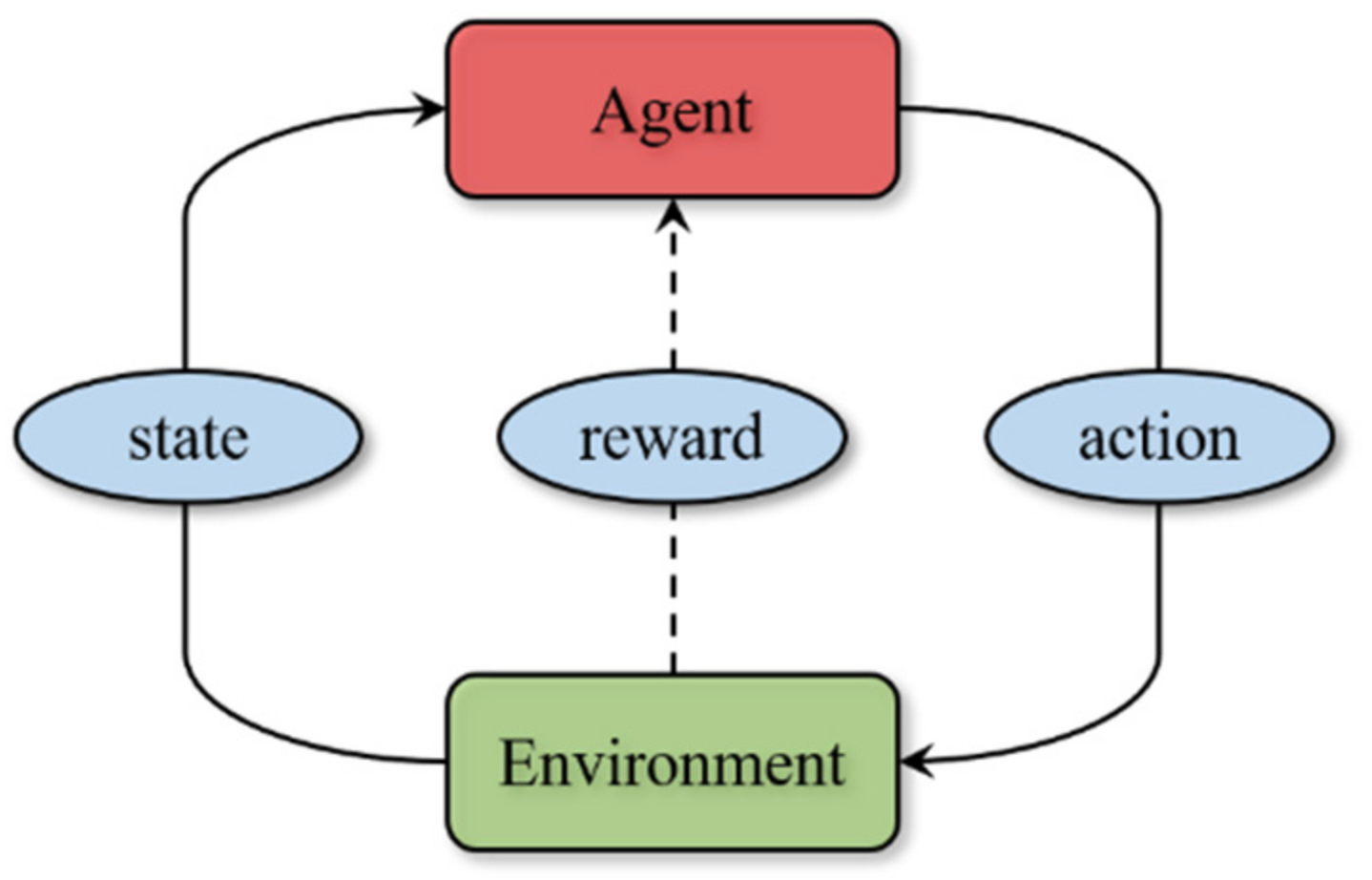
3. Maneuver Decision Method Based on a Proximal Policy Optimization Algorithm

3.1. Proximal Policy Optimization Algorithm

Reinforcement learning is a branch of machine learning [25]. Different from supervised learning and unsupervised learning, the agent in reinforcement learning learns strategy by interaction with the environment. The general model of reinforcement learning is the Markov decision process (MDP), which is shown in Figure 10. The model is composed of an environment, agent, state, reward and action. The environment includes the motion law of the object and some restrictions. It receives the action and updates the state and feeds back the reward to the agent. The agent is the carrier of reinforcement learning algorithm, which outputs the action according to the state of the environment and the reward.

At each step, the agent executes action $a_t$ according to the policy $\pi$, and then the state of the agent updates from $s_t$ to $s_{t+1}$ with the state transition probability $p\left(s_{t+1}\left|s_t,a_t\right.\right)$. The environment feedbacks reward $r\left(s_t,a_t\right)$ to the agent at the same time. The goal of reinforcement learning is to determine the optimal strategy ${\pi }^{\ast }$ to maximize the expected discount cumulative return, $V^{\pi }\left(s\right)$, called the value function [25], which is defined as:

$$V^{\pi }\left(s\right)={\mathbb{E}}_{s_t,a_t~\pi }\left[{\displaystyle \sum _{t=0}^{\infty }{\tau }^{t}r\left(s_t,a_t\right)}\right],$$

(17)

where $\tau \in \left(0,1\right)$ denotes the discount factor. Therefore, the optimal value function, $V^{*}\left(s\right)$ (i.e., the maximum value of the expected discount cumulative return), is defined as:

$$V^{*}\left(s\right)=\max {\mathbb{E}}_{s_t,a_t~{\pi }^{*}}\left[{\displaystyle \sum _{t=0}^{\infty }{\tau }^{t}r\left(s_t,a_t\right)}\right],$$

(18)

Deep reinforcement learning is a combination of deep learning and reinforcement learning, which uses the parameter $\theta$ of neural networks to store and update the policy ${\pi }_{\theta }$ of reinforcement learning. It has an edge in solving the problems with high task complexity, high dimension of solution space and redundant state information.

The proximal policy optimization algorithm (PPO) is an on-policy algorithm based on policy gradient methods [26] for deep reinforcement learning. Policy gradient methods work by computing an estimator of the policy gradient and plugging it into a stochastic gradient ascent algorithm. The loss function of a PPO is defined as [22]:

$$L_t^{CLIP+VF+S}\left(\theta \right)={\widehat{\mathbb{E}}}_t\left[L_t^{CLIP}\left(\theta \right)-c_1{L}_t^{VF}\left(\theta \right)+c_{2}S\left[{\pi }_{\theta }\right]\left(s_t\right)\right],$$

(19)

where $c_1$ and $c_2$ are coefficients; $L^{VF}\left(\theta \right)$ is the value function of the squared-error loss; $S\left[{\pi }_{\theta }\right]$ denotes the entropy bonus of policy ${\pi }_{\theta }$ [27,28]. The surrogate objective $L^{CLIP}\left(\theta \right)$ is the core of the PPO algorithm, which is defined as [22]:

$$L^{CLIP}\left(\theta \right)={\widehat{\mathbb{E}}}_t\left[\min \left(r_t\left(\theta \right){\widehat{A}}_t{,}^{}\mathrm{clip}\left(r_t\left(\theta \right){,}^{}1-\epsilon ,1+\epsilon \right){\widehat{A}}_t\right)\right],$$

(20)

$$r_t\left(\theta \right)=\frac{{\pi }_{\theta }\left(a_t\left|s_t\right.\right)}{{\pi }_{{\theta }_{\mathrm{old}}}\left(a_t\left|s_t\right.\right)},$$

(21)

where $\epsilon$ denotes the clip range, which is used to clip the probability ratio $r_t\left(\theta \right)$ to avoid an excessively large policy update; ${\widehat{A}}_t$ is an estimator of the advantage function, which can be calculated by generalized advantage estimation (GAE) [29].

$${\widehat{A}}_t={\displaystyle \sum _{l=0}^{\infty }{\left(\tau \lambda \right)}^l{\delta }_{t+l}^V},$$

(22)

where $\lambda$ is the GAE factor, and ${\delta }_t^V$ is defined as [29]:

$${\delta }_t^V=r_t+\tau V\left(s_{t+1}\right)-V\left(s_t\right),$$

(23)

In the training process, the PPO algorithm updates the parameter $\theta$ of the neural network by optimizing the loss function $L_t^{CLIP+VF+S}\left(\theta \right)$ to achieve the purpose of updating the policy.

3.2. Action Space

The action space is divided into discrete space and continuous space. The discrete action space, ${\mathit{A}}_1$, can be directly composed of the basic maneuver library in Table 1, which is expressed as ${\mathit{A}}_1=\left[{\mathit{a}}_1,{\mathit{a}}_2,\cdots ,{\mathit{a}}_{13}\right]$. The discrete action space, based on the maneuver library, is equivalent to providing priori experience for the agent. Compared with the discrete action space, the continuous action space, ${\mathit{A}}_2$, can make better use of the maneuverability of a UCAV, but it may increase the difficulty of flight control and reduce the learning efficiency. Since the actions of reinforcement learning generally need to be normalized, it was necessary to linearly map the control input $\mathit{u}$. Therefore, the continuous action space ${\mathit{A}}_2$ can be expressed as:

$${\mathit{A}}_2=\left\{\mathit{a}\left|\mathit{a}=f\left(\mathit{u}\right){,}_{}{\mathit{a}}_j\in \left[-1,1\right]{,}_{}\hspace{1em}j=1,2,3\right.\right\},$$

(24)

where $f\left(\cdot \right)$ denotes linear mapping; ${\mathit{a}}_j$ denotes the jth dimension element of action $\mathit{a}$.

A comparative experiment between the discrete action space and the continuous action space is carried out in Section 4.

3.3. State Observation Space

The convergence of the algorithm is affected by the state observation space. Design of the state observation space strives to be concise and efficient. On the one hand, incompleteness of information in the state observation space may make the algorithm difficult to converge. On the other hand, redundant information in the state observation may cause overfitting. In addition, refining the original state information properly and designing the information highly relevant to decisions can reduce the training time. Therefore, a 14-dimensional state observation space is designed in this section, and the information was scaled to facilitate feature extraction with a neural network.

Taking the red UCAV as an example, the state observation space $\mathit{S}=\left[s_1,s_2,\cdots ,s_{14}\right]$ is shown in

Table 2. State observation space.

State	Value	State	Value
$s_1$	$x_r/x_{\max }$	$s_8$	$x_b/x_{\max }$
$s_2$	$y_r/y_{\max }$	$s_9$	$y_b/y_{\max }$
$s_3$	$z_r/z_{\max }$	$s_{10}$	$z_b/z_{\max }$
$s_4$	$‖{\mathit{v}}_r‖/v_{\max }$	$s_{11}$	$‖{\mathit{v}}_b‖/v_{\max }$
$s_5$	$v_r^x/v_{\max }$	$s_{12}$	$v_b^x/v_{\max }$
$s_6$	$v_r^y/v_{\max }$	$s_{13}$	$v_b^y/v_{\max }$
$s_7$	$v_r^z/v_{\max }$	$s_{14}$	$v_b^z/v_{\max }$

.

3.4. Reward Function with Situation Reward Shaping

The design of the reward function is one of the keys to deciding whether the algorithm is convergent. Only when the UCAV of one side dies can victory or defeat be determined in air combat, which can be abstracted as a sparse reward problem in reinforcement learning. The sparse reward problem means that the agent finds it difficult to learn tasks with high exploration complexity due to the lack of a feedback signal [30]. In order to make the algorithm converge within a limited time, a reward function with situation reward shaping based on air combat situation assessment is designed in this section. The design using the air combat situation assessment can make the reward function continuous. The idea of situation reward shaping is to design the reward by the state situation of the agent, so that the agent will explore the terminal state faster to experience less punishment. The situation guidance reward is defined as:

$$B_{situ}=\frac{‖{\mathit{v}}_r‖\cos (ATA)}{v_{\max }},$$

(25)

The situation guidance reward reflects the current state of the UCAV. When the reward is positive, the UCAV is in an offensive situation, and when the reward is negative, the UCAV is in a defensive situation.

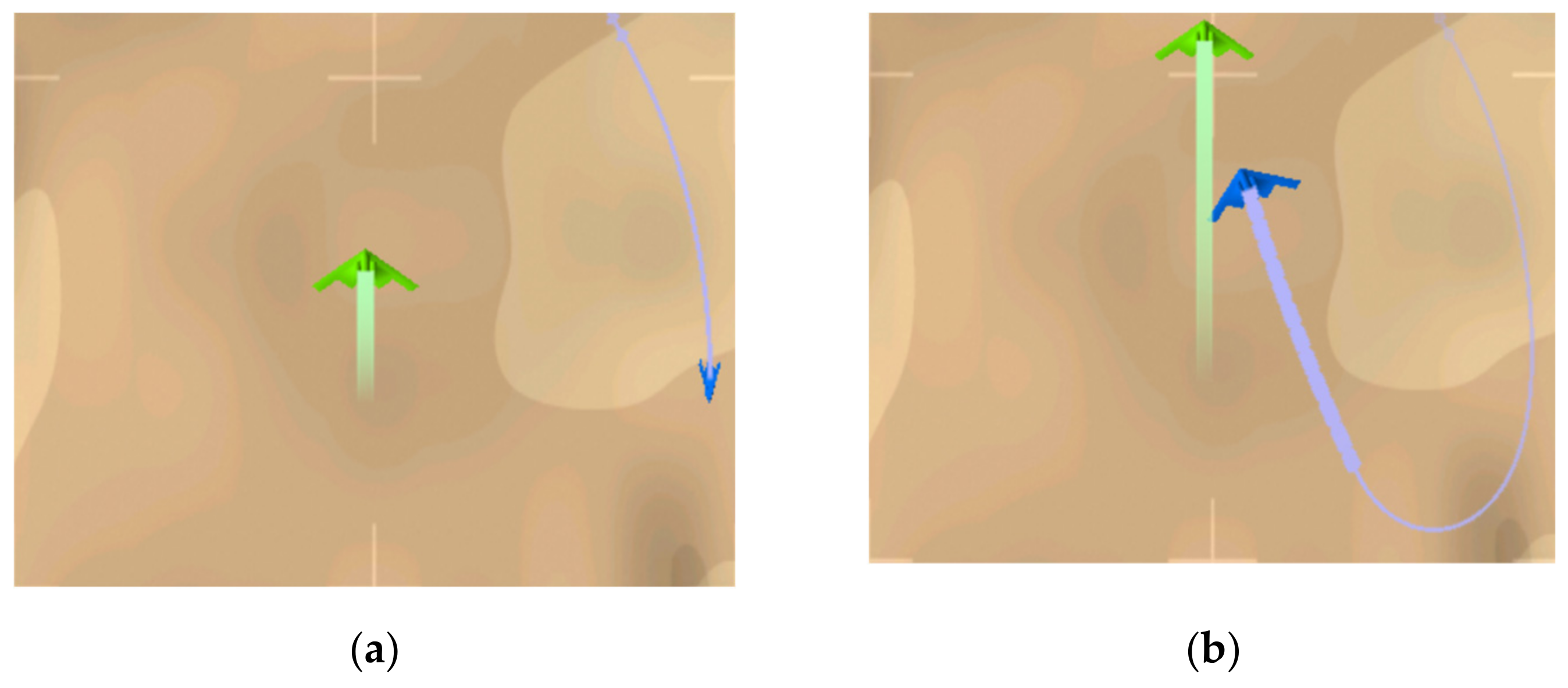
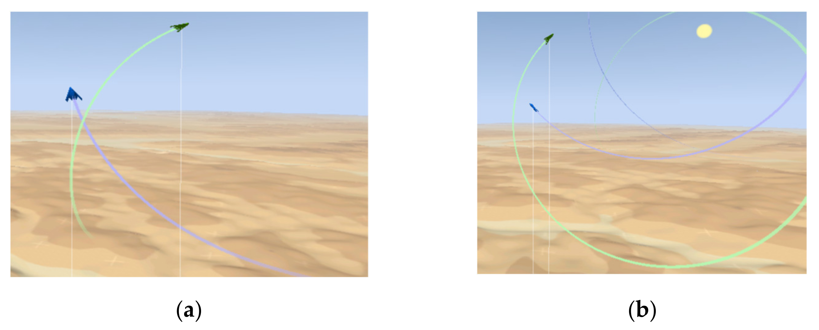
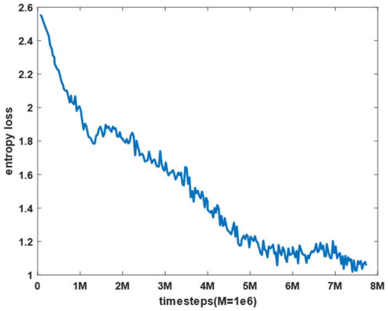
4. Simulation Results

4.1. Simulation Platform

The simulation environment in this paper was built with Python, and the algorithm was implemented based on PyTorch. The real-time confrontation display was based on Tacview. The experimental equipment was a desktop computer configured with an Intel(R) Xeon(R) Gold 6254 CPU @ 3.10 GHz and a single NVIDIA GeForce RTX 3090 GPU.

In order to ensure the fairness of the confrontation, the blue UCAV adopted the same parameters as the red UCAV. The relevant parameter settings are shown in

Table 3. Relevant parameters of air combat.

Parameter	Value	Parameter	Value
$\alpha$	$\pi /3$	$t_{\max }$	3 × 103
$R_{\min }$	500	$k_v$	20
$R_{\max }$	2 × 103	$k_h$	500
$v_{\min }$	100	$k_d$	2 × 103
$h_{\min }$	2 × 103	$d_{\mathrm{threshold}}$	8 × 103

.

After debugging, the relevant parameters of deep reinforcement learning, including neural network parameters, were set as follows. The policy network and value network were constructed by a fully connected network. Both of the networks had two hidden layers with 64 and 64 units, respectively. The activation function was a tanh function. The PPO algorithm used eight environments to collect data in parallel in the simulation. The number of steps to run for each environment per update was 4096, the minibatch size was 128 and the number of epoch when optimizing the surrogate loss was 10. The discount factor $\tau =0.99$, the value function squared-error loss coefficient $c_1=0.5$, the entropy bonus coefficient $c_2=0.001$, the clip range $\epsilon =0.2$ and the GAE factor $\lambda =0.95$.

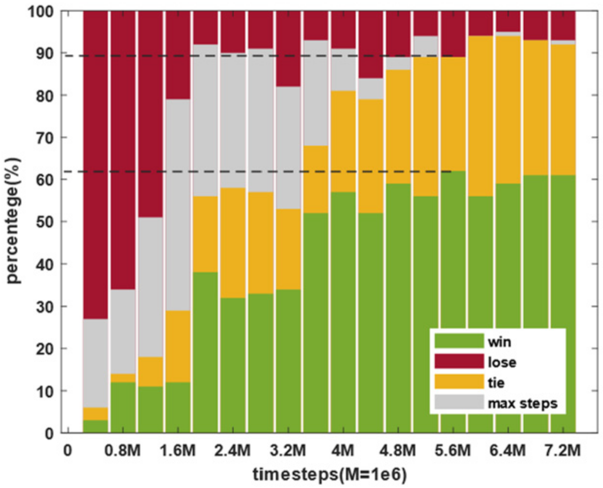
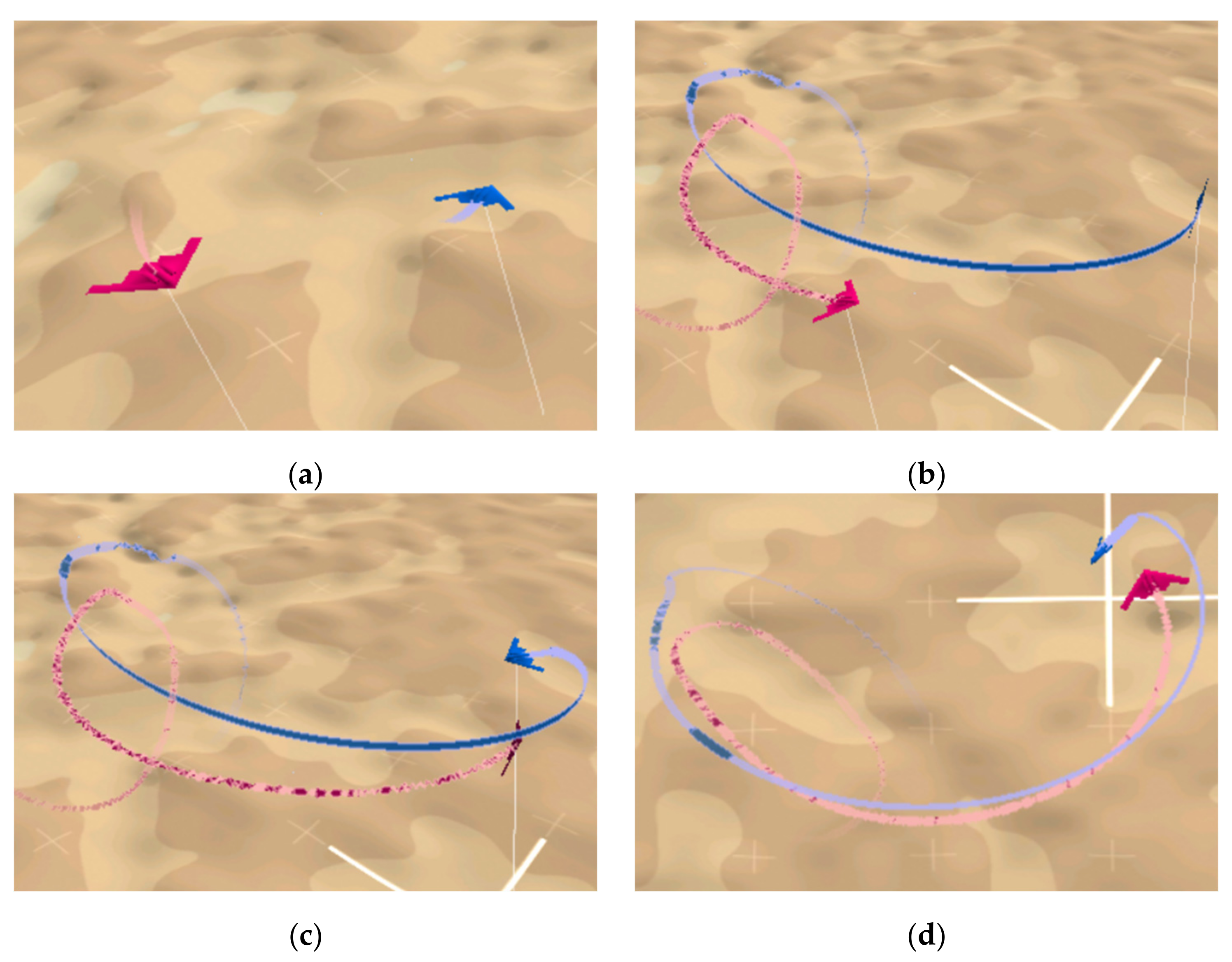
4.2. Results and Analysis

Figure 11 and Figure 12 show that the different stages of the blue UCAV with the greedy algorithm chasing the green target moving in the horizontal plane and vertical plane, respectively. It can be seen from Figure 11 and Figure 12 that the blue UCAV shot down the green target successfully through a series of maneuvers such as turn and climb. Moreover, the blue UCAV also had the ability to avoid entering the attack zone of the target, which verifies the effectiveness of the maneuver strategy based on the greedy algorithm.

In order to ensure the fairness of the confrontation and to be consistent with an actual combat environment, the position, velocity and attitude of the UCAVs were initialized stochastically within a certain range in the training process. The initial states settings of the UCAVs are shown in

Table 4. Initial states setting.

State	Value	State	Value
$x$	[−10, 10] km	$v$	[100, 600] m/s
$y$	[−10, 10] km	$\gamma$	[−$\pi$/2, $\pi$/2] rad
$z$	[−12, −8] km	$\psi$	[−$\pi$,$\pi$] rad

.

Figure 13 shows the training curve of the agents with different action spaces. The horizontal axis is the number of training time steps, and the vertical axis is the average reward value of each episode in the rollout of the PPO algorithm, which reflects the convergence of the training. As can be seen from Figure 13, the agent using discrete action space quickly improved the average reward per episode and stabilized at approximately 300. However, the agent using continuous action space had no prior experience and needed to learn flight control first. Therefore, the average reward increased slowly and only stabilized at approximately 50 in the later stage. The subsequent experiments in this paper used the discrete action space.

Figure 14 shows the average steps of the agent in each episode during the training process. It can be seen from the figure that the average length of the episode increased gradually in the early stage of the training but decreased gradually when the number of training time steps was greater than 2 M, and it finally stabilized at approximately 700 steps. In addition, the average reward value of per episode in Figure 13 tended to rise first and then stabilize, which shows that the average reward received by the agent at each step gradually increased.

Figure 15 and Figure 16 show the entropy loss and the explained variance of the PPO algorithm during the training process, respectively. The entropy loss reflects the randomness of the actions of the agent. As can be seen from Figure 15, the entropy loss gradually dropped to a lower level after the beginning of training, which indicates that the policy of the agent was relatively stable in the later stage of training. The explained variance reflects the fitting accuracy of the value network of the PPO algorithm. The closer it is to one, the higher the accuracy. It can be seen from Figure 16 that the explained variance rose rapidly in the beginning of training and increased with the training time steps, and it finally stabilized at approximately one. Figure 15 and Figure 16 show that the performance of the policy network of the agent converged to a high level after the training.

Figure 17 shows the results of 100 episodes of air combat confrontation between the agent and the blue UCAV based on the greedy policy. The confrontation results are divided into four types including winning, losing, drawing and reaching the maximum number of steps in the current episode. Winning means that the UCAV shot down the enemy, or the enemy went beyond the margins. Losing means that the enemy shot down the UCAV, or the UCAV went beyond the margins. Drawing means that the two UCAVs met the firing conditions at the same time and were shot down by the other side, or the two the UCAVs went beyond the margins. The horizontal axis is the number of training steps, and the vertical axis is the percentage of the results. Green represents winning, red represents losing, yellow represents a tie, and grey represents that the current episode reached the maximum number of steps. As can be seen from Figure 17, the winning rate of the agent gradually rose with the increase in the number of training time steps and tended to be stable. After training, the winning rate can reach 62%, and the corresponding losing rate is only 11%. In addition, the average decision time per step of the PPO algorithm was 0.98 ms and that of the greedy algorithm was 1.62 ms, both of which were less than the simulation step size of 0.1 s, thus meeting the real-time requirements. It should be pointed out that even in the later stage of training, the greedy algorithm could still maintain a certain unbeaten rate for the blue UCAV, which shows that it also had a strong autonomous decision ability.

Figure 14 and Figure 17 show that the agent lacked attack skills in the early stage of training, but learned to avoid attack from the blue UCAV so as to increase the cumulative reward by prolonging the survival steps. As a result, the agent in the early stage of training often reached the maximum number of steps. When the training reached a certain level, the agent gradually learned the attack skills, which could not only defeat the blue UCAV but also reduce the maneuver time steps. The above conditions show that the maneuver decision method proposed in this paper can enable a UCAV to learn the maneuver policy autonomously and defeat the enemy.

The experiments in this paper realized real-time situation display through a TCP communication protocol and Tacview software. Figure 18 is an example of the real-time display. Figure 19 displays the recorded trajectory curves of the two UCAVs for the example in Figure 18. As can be seen from Figure 18 and Figure 19, the agent had learned to combine a series of basic maneuvers, such as diving, climbing and circling, into tactical maneuvers and finally defeated the enemy.

5. Conclusions

In this paper, a UCAV air combat maneuver decision method based on a PPO algorithm was proposed. Firstly, a general UAV short-range air combat confrontation framework was established including a motion model of a fixed-wing aircraft and a situation assessment model of air combat. In order to verify the effectiveness of the method, an enemy maneuver strategy based on a greedy algorithm was designed. Then, the action space based on a basic maneuver library and a state observation space for the agent were constructed. A maneuver policy was generated by training with the PPO algorithm. A reward function based on situation reward shaping was designed for accelerating the convergence rate of the algorithm. Finally, simulations of one-to-one, short-range air combat in stochastic situations were carried out to verify the effectiveness of the PPO algorithm. The experiment with agents using different action spaces showed that the discrete action space may reduce the difficulty of flight control and increase the learning efficiency. The experiment with the blue UCAV using a greedy algorithm to chase a moving target resulting in 100 episodes of air combat confrontation showed that the greedy algorithm also has a strong autonomous decision ability, but the performance of the PPO algorithm was better. The winning rate of the PPO algorithm reached 62%, and the corresponding losing rate was only 11%. In addition, the average decision time per step of the PPO algorithm was less than the simulation step size of 0.1 s, meeting real-time requirements. As can be seen from the real-time display example, the agent learned to combine a series of basic maneuvers, such as diving, climbing and circling, into tactical maneuvers. The results of the simulations show that the maneuver decision method proposed in this paper can enable a UCAV to learn the maneuver policy autonomously and defeat the enemy.

In addition, the proposed UCAV maneuver decision method is essentially motion control of a UAV. Therefore, it also has application potential in other fields including monitoring, organizing communication, search and transportation [31,32,33].

References

1. McManus, J.W.; Chappell, A.R.; Arbuckle, P.D. Situation Assessment in the Paladin Tactical Decision Generation System. In AGARD Conference AGARD-CP-504: Air Vehicle Mission Control and Management; NATO: Amsterdam, The Netherlands, 1992. [Google Scholar]
2. Burgin, G.H. Improvements to the Adaptive Maneuvering Logic Program; NASA CR-3985; NASA: Washington, DC, USA, 1986. [Google Scholar]
3. Ernest, N.; Carroll, D.; Schumacher, C.; Clark, M.; Cohen, K.; Lee, G. Genetic Fuzzy based Artificial Intelligence for Unmanned Combat Aerial Vehicle Control in Simulated Air Combat Missions. J. Def. Manag. 2016, 6, 1–7. [Google Scholar] [CrossRef]
4. DARPA. Air Combat Evolution. Available online: https://www.darpa.mil/program/air-combat-evolution (accessed on 24 June 2022).
5. Vajda, S. Differential Games. A Mathematical Theory with Applications to Warfare and Pursuit, Control and Optimization. By Rufus Isaacs. Pp. xxii, 384. 113s. 1965. (Wiley). Math. Gaz. 1967, 51, 80–81. [Google Scholar] [CrossRef]
6. Mendoza, L. Qualitative Differential Equations. Dict. Bioinform. Comput. Biol. 2004, 68, 421–430. [Google Scholar] [CrossRef]
7. Park, H.; Lee, B.-Y.; Tahk, M.-J.; Yoo, D.-W. Differential Game Based Air Combat Maneuver Generation Using Scoring Function Matrix. Int. J. Aeronaut. Space Sci. 2016, 17, 204–213. [Google Scholar] [CrossRef]
8. Bullock, H.E. ACE: The Airborne Combat Expert Systems: An Exposition in Two Parts. Master’s Thesis, Defense Technical Information Center, Fort Belvoir, VA, USA, 1986. [Google Scholar]
9. Chin, H.H. Knowledge-based system of supermaneuver selection for pilot aiding. J. Aircr. 1989, 26, 1111–1117. [Google Scholar] [CrossRef]
10. Wang, R.; Gao, Z. Research on Decision System in Air Combat Simulation Using Maneuver Library. Flight Dyn. 2009, 27, 72–75. [Google Scholar]
11. Xuan, W.; Weijia, W.; Kepu, S.; Minwen, W. UAV Air Combat Decision Based on Evolutionary Expert System Tree. Ordnance Ind. Autom. 2019, 38, 42–47. [Google Scholar]
12. Huang, C.; Dong, K.; Huang, H.; Tang, S.; Zhang, Z. Autonomous air combat maneuver decision using Bayesian inference and moving horizon optimization. J. Syst. Eng. Electron. 2018, 29, 86–97. [Google Scholar] [CrossRef]
13. Cao, Y.; Kou, Y.-X.; Xu, A.; Xi, Z.-F. Target Threat Assessment in Air Combat Based on Improved Glowworm Swarm Optimization and ELM Neural Network. Int. J. Aerosp. Eng. 2021, 2021, 4687167. [Google Scholar] [CrossRef]
14. Kaneshige, J.; Krishnakumar, K. Artificial immune system approach for air combat maneuvering. In Proceedings of the SPIE 6560, Intelligent Computing: Theory and Applications V, Orlando, FL, USA, 9–13 April 2007; Volume 6560, p. 656009. [Google Scholar] [CrossRef]
15. Başpinar, B.; Koyuncu, E. Assessment of Aerial Combat Game via Optimization-Based Receding Horizon Control. IEEE Access 2020, 8, 35853–35863. [Google Scholar] [CrossRef]
16. François-Lavet, V.; Henderson, P.; Islam, R.; Bellemare, M.G.; Pineau, J. An Introduction to Deep Reinforcement Learning. Found. Trends Mach. Learn. 2018, 11, 219–354. [Google Scholar] [CrossRef]
17. McGrew, J.S.; How, J.; Williams, B.C.; Roy, N. Air-Combat Strategy Using Approximate Dynamic Programming. J. Guid. Control Dyn. 2010, 33, 1641–1654. [Google Scholar] [CrossRef]
18. Liu, P.; Ma, Y. A Deep Reinforcement Learning Based Intelligent Decision Method for UCAV Air Combat. In Modeling, Design and Simulation of Systems, Proceedings of the 17th Asia Simulation Conference, AsiaSim 2017, Malacca, Malaysia, 27–29 August 2017; Communications in Computer and Information Science; Springer: Singapore, 2017; pp. 274–286. [Google Scholar] [CrossRef]
19. Zhang, X.; Liu, G.; Yang, C.; Wu, J. Research on Air Confrontation Maneuver Decision-Making Method Based on Reinforcement Learning. Electronics 2018, 7, 279. [Google Scholar] [CrossRef]
20. Yang, Q.; Zhang, J.; Shi, G.; Hu, J.; Wu, Y. Maneuver Decision of UAV in Short-Range Air Combat Based on Deep Reinforcement Learning. IEEE Access 2019, 8, 363–378. [Google Scholar] [CrossRef]
21. Kong, W.; Zhou, D.; Yang, Z.; Zhao, Y.; Zhang, K. UAV Autonomous Aerial Combat Maneuver Strategy Generation with Observation Error Based on State-Adversarial Deep Deterministic Policy Gradient and Inverse Reinforcement Learning. Electronics 2020, 9, 1121. [Google Scholar] [CrossRef]
22. Schulman, J.; Wolski, F.; Dhariwal, P.; Radford, A.; Klimov, O. Proximal Policy Optimization Algorithms. arXiv 2017, arXiv:1707.06347. [Google Scholar]
23. Hu, J.; Wang, L.; Hu, T.; Guo, C.; Wang, Y. Autonomous Maneuver Decision Making of Dual-UAV Cooperative Air Combat Based on Deep Reinforcement Learning. Electronics 2022, 11, 467. [Google Scholar] [CrossRef]
24. Austin, F.; Carbone, G.; Falco, M.; Hinz, H.; Lewis, M. Automated maneuvering decisions for air-to-air combat. In Proceedings of the Guidance, Navigation and Control Conference, Monterey, CA, USA, 17–19 August 1987. [Google Scholar] [CrossRef]
25. Sutton, R.S.; Barto, A.G. Reinforcement Learning: An Introduction; MIT Press: Cambridge, MA, USA, 2018. [Google Scholar]
26. Paczkowski, M. Low-Friction Composite Creping Blades Improve Tissue Properties. In Proceedings of the Pulp and Paper, Stockholm, Sweden, 9 October 1996; Volume 70. [Google Scholar]
27. Williams, R.J. Simple Statistical Gradient-Following Algorithms for Connectionist Reinforcement Learning. Mach. Learn. 1992, 8, 229–256. [Google Scholar] [CrossRef]
28. Mnih, V.; Badia, A.P.; Mirza, L.; Graves, A.; Lillicrap, T.; Harley, T.; Silver, D.; Kavukcuoglu, K. Asynchronous Methods for Deep Reinforcement Learning. In Proceedings of the 33rd International Conference on Machine Learning, ICML 2016, New York, NY, USA, 19–24 June 2016; Volume 48, pp. 1928–1937. [Google Scholar]
29. Schulman, J.; Moritz, P.; Levine, S.; Jordan, M.; Abbeel, P. High-Dimensional Continuous Control Using Generalized Advantage Estimation. In Proceedings of the 4th International Conference on Learning Representations, ICLR 2016–Conference Track Proceedings, San Juan, Puerto Rico, 2–4 May 2016; pp. 1–14. [Google Scholar]
30. Riedmiller, M.; Hafner, R.; Lampe, T.; Neunert, M.; Degrave, J.; Van De Wiele, T.; Mnih, V.; Heess, N.; Springenberg, J.T. Learning by Playing Solving Sparse Reward Tasks from Scratch. In Proceedings of the 35th International Conference on Machine Learning, ICML 2018, Stockholm, Sweden, 10–15 July 2018; Volume 80, pp. 4344–4353. [Google Scholar]
31. Mukhamediev, R.I.; Symagulov, A.; Kuchin, Y.; Zaitseva, E.; Bekbotayeva, A.; Yakunin, K.; Assanov, I.; Levashenko, V.; Popova, Y.; Akzhalova, A.; et al. Review of Some Applications of Unmanned Aerial Vehicles Technology in the Resource-Rich Country. Appl. Sci. 2021, 11, 10171. [Google Scholar] [CrossRef]
32. Agarwal, A.; Kumar, S.; Singh, D. Development of Neural Network Based Adaptive Change Detection Technique for Land Terrain Monitoring with Satellite and Drone Images. Def. Sci. J. 2019, 69, 474–480. [Google Scholar] [CrossRef]
33. Smith, M.L.; Smith, L.N.; Hansen, M.F. The quiet revolution in machine vision–A state-of-the-art survey paper, including historical review, perspectives, and future directions. Comput. Ind. 2021, 130, 103472. [Google Scholar] [CrossRef]
Figure 1. UCAV motion model.
Electronics 11 02602 g001
Figure 2. Geometry of air combat.
Electronics 11 02602 g002
Figure 3. Attack zone of a UCAV.
Electronics 11 02602 g003
Figure 4. Top view of the attack zone.
Electronics 11 02602 g004
Figure 5. (a) Velocity index; (b) altitude index.
Electronics 11 02602 g005
Figure 6. Change in η 2 with the distance between two UCAVs.
Electronics 11 02602 g006
Figure 7. Change in η 3 with A A .
Electronics 11 02602 g007
Figure 8. Change in η 4 with the distance between two UCAVs.
Electronics 11 02602 g008
Figure 9. Air combat situation at the same altitude: (a) stereoscopic view of the air combat situation at the same altitude; (b) plan view of the air combat situation at the same altitude.
Electronics 11 02602 g009
Figure 10. General model of reinforcement learning.
Electronics 11 02602 g010
Figure 11. Blue UCAV chasing the green target moving in the horizontal plane: (a) early stage of air combat; (b) later stage of air combat.
Electronics 11 02602 g011
Figure 12. Blue UCAV chasing the green target moving in the vertical plane: (a) early stage of air combat; (b) later stage of air combat.
Electronics 11 02602 g012
Figure 13. Training curve of the agents using different action spaces.
Electronics 11 02602 g013
Figure 14. Mean length per episode in the training process.
Electronics 11 02602 g014
Figure 15. Entropy loss of the PPO algorithm in the training process.
Electronics 11 02602 g015
Figure 16. Explained variance of the PPO algorithm in the training process.
Electronics 11 02602 g016
Figure 17. Air combat confrontation results.
Electronics 11 02602 g017
Figure 18. Real-time display example of air combat confrontation: (a) early stage of air combat; (b) medium stage of air combat; (c) later stage of air combat; (d) top view of the air combat.
Electronics 11 02602 g018
Figure 19. Trajectories for the air combat confrontation example: (a) two UCAVs; (b) top view of the two UCAVs; (c) altitudes of the two UCAVs.
Electronics 11 02602 g019