Optimized Deep Learning Algorithms for Tomato Leaf Disease Detection with Hardware Deployment

Abstract

Smart agriculture has taken more attention during the last decade due to the bio-hazards of climate change impacts, extreme weather events, population explosion, food security demands and natural resources shortage. The Egyptian government has taken initiative in dealing with plants diseases especially tomato which is one of the most important vegetable crops worldwide that are affected by many diseases causing high yield loss. Deep learning techniques have become the main focus in the direction of identifying tomato leaf diseases. This study evaluated different deep learning models pre-trained on ImageNet dataset such as ResNet50, InceptionV3, AlexNet, MobileNetV1, MobileNetV2 and MobileNetV3.To the best of our knowledge MobileNetV3 has not been tested on tomato leaf diseases. Each of the former deep learning models has been evaluated and optimized with different techniques. The evaluation shows that MobileNetV3 Small has achieved an accuracy of 98.99% while MobileNetV3 Large has achieved an accuracy of 99.81%. All models have been deployed on a workstation to evaluate their performance by calculating the prediction time on tomato leaf images. The models were also deployed on a Raspberry Pi 4 in order to build an Internet of Things (IoT) device capable of tomato leaf disease detection. MobileNetV3 Small had a latency of 66 ms and 251 ms on the workstation and the Raspberry Pi 4, respectively. On the other hand, MobileNetV3 Large had a latency of 50 ms on the workstation and 348 ms on the Raspberry Pi 4.

1. Introduction

In the last few years, climate change impacts on food production and human life have become more serious regarding the huge changes in humans lifestyle, urbanization, natural resources shortages. The large increase in population densities has led to the increase of food security and safety demands. The need to increase food production and mitigate or adapt to the climate change impacts on the agricultural field were the driving force for integrating the smart system in agriculture production. Based on [1], 690 million people around the world are suffering from hunger and more than 200 million had malnutrition. Agri-food production systems are requesting to increase food production with sustainable action to match the Sustainable Development Goals (SDG).

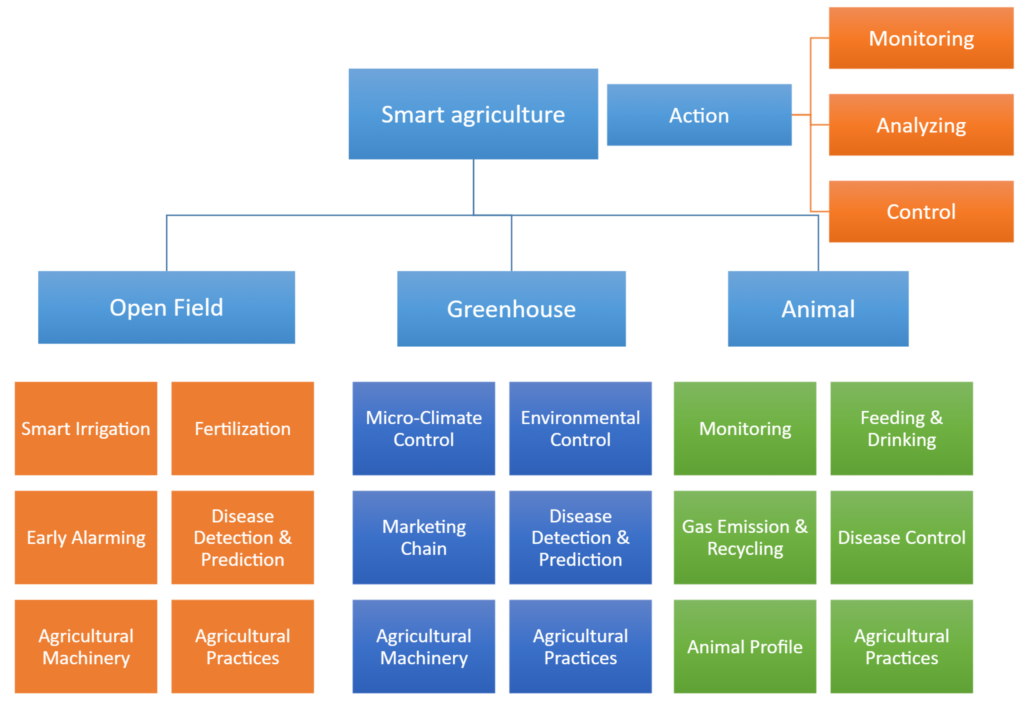
Smart agriculture utilizes technologies such as sensors, robotics, IoT and artificial intelligence (AI). The rapid development in the field of IoT [2] has supported the revolution of smart agriculture and its ability to be deployed in the open field and the greenhouse. It is implemented by collecting data from sensors then the data are diagnosed and analyzed by the system to identify anomalies. Based on the problems identified, the utilized platform decides the action that needs to be taken to solve them. There are many applications concerning the smart agriculture field such as smart irrigation, agricultural machinery, disease detection in the open field and micro-climate control, environmental control and marketing chain in the smart greenhouse. The applications of smart agriculture are summarized in Figure 1 concluded from Food and Agriculture Organization of the United Nations (FAO) Catalogue, 2021 [1].

Figure 1. Applications of Smart Agriculture Based on [1].

Kodali, Ravi et al. [3] studied the improvement of agricultural practices by providing a model of a smart greenhouse to eliminate the use of manual inspection and monitoring the plants’ environmental conditions which helped reduce 80% of the water waste and provide climate control to ensure proper growth for these plants.

Wiangtong, Theerayod et al. [4] developed a controller to monitor data such as temperature and humidity and send them to clients via the internet while the hardware take decisions to regulate temperature and humidity.

Awan, Kamran et al. [5] proposed a time-driven trust management mechanism to secure the data transmitted from the sensors to the cloud by identifying malicious nodes that can affect secure environments.

Nowadays, the current Egyptian government has taken revolutionary steps to digitize most of the governmental services sectors such as health, traffic and agriculture. They started deploying IoT systems including sensors to measure the humidity and moisture of the soil and then the data are transmitted to farmers’ phones via satellite signals and the farmer would be able to irrigate his land while staying at home. This initiative will help regulate the irrigation process which will lead to a drastic reduction of water waste and increase crops productivity.

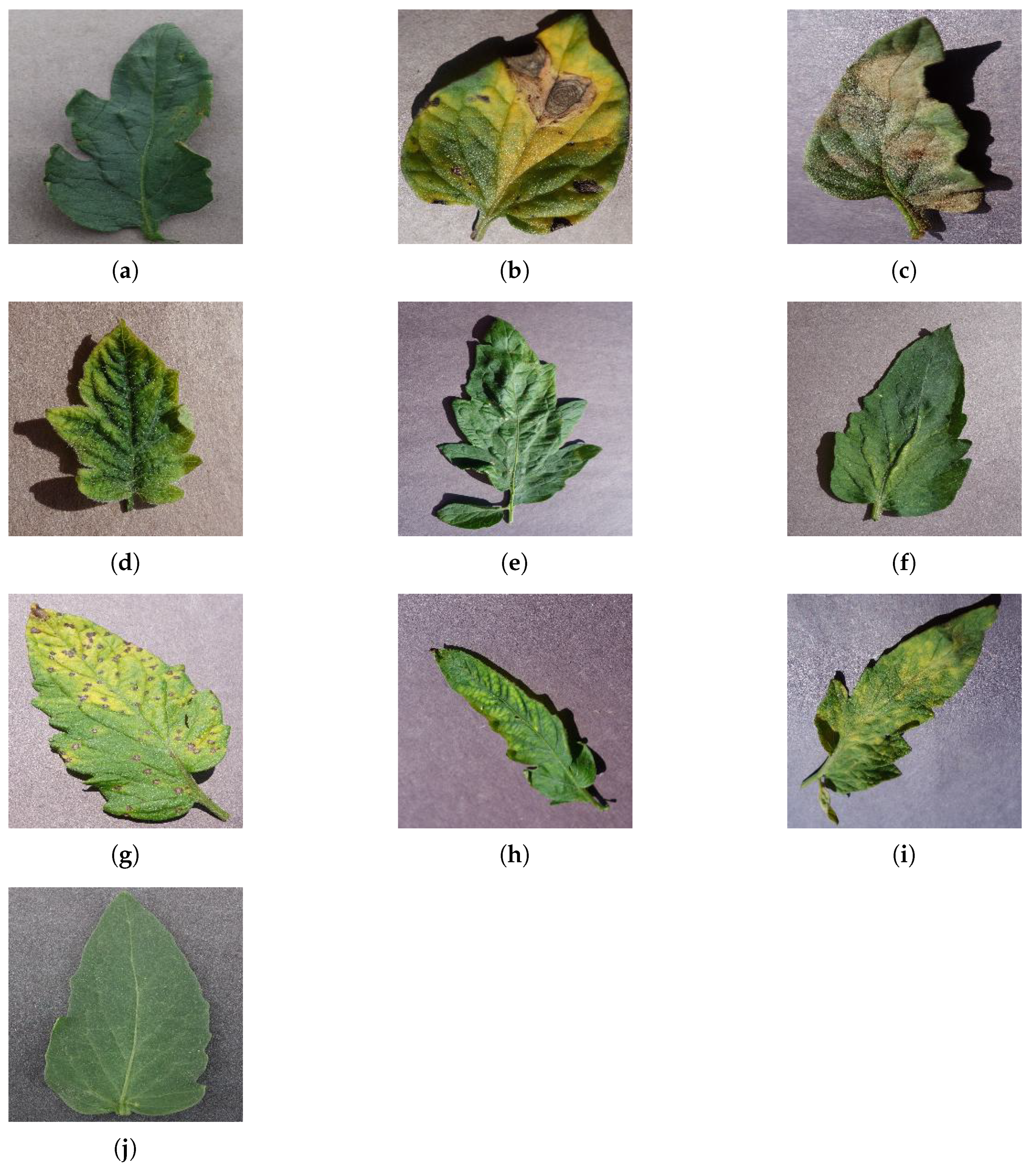
Climate change has severely impacted the crops yield and quality in Egypt. The most destructive plant diseases (Potato Late Blight, Tomato Late Blight) have expanded in the last few decades in response to climate change [6]. Tomato is the most important vegetable in terms of world production and consumption [7]. Egypt is the fifth worldwide producer of tomatoes after India, the United States, China and Turkey. These countries represent 62% of the world’s tomato production. The main reasons for yield decrease in tomato production are the diseases affecting the plants which start from the leaves then spread to the entire plant [8]. To date, farmers in Egypt rely on human inspection to identify tomato leaf diseases which can lead to a huge waste of time and a large probability of error. The need for using new technologies such as Artificial Intelligence (AI) and Computer Vision (CV) arises in the efforts to improve the plant disease detection procedure.

The field of artificial intelligence and computer vision has seen an immense surge due to its ability of image recognition and classification [9]. Machine learning and deep learning are both subcategories of AI [10]. Machine learning is the process of training machines to be able to perform certain tasks without the need of explicit programming. Deep learning is a subset of machine learning [11] and is based on neural networks, it can be based on supervised or unsupervised learning [12]. Deep learning has become more popular recently due to its large variety of applications in the field of computer vision and natural language processing. The word “deep” in deep learning refers to the large number of layers that are embedded into the models. Unlike machine learning, deep learning models have the ability to extract features on its own without the need for a human to make adjustments or choose these features. Among many of deep learning structures, A convolutional neural network (CNN) is a type of deep learning model that is widely used in image classification due to its ability to automatically and adaptively learn features [13]. A CNN normally consists of three types of layers: convolutional layer, pooling layer and fully-connected layer [14]. The first two layers, convolutional and pooling are the layers responsible for the feature extraction of the images while the fully connected layer transforms the extracted features into image classification. Image classification is the process of inspecting a certain image and predicting the class to which the image belongs to [15].

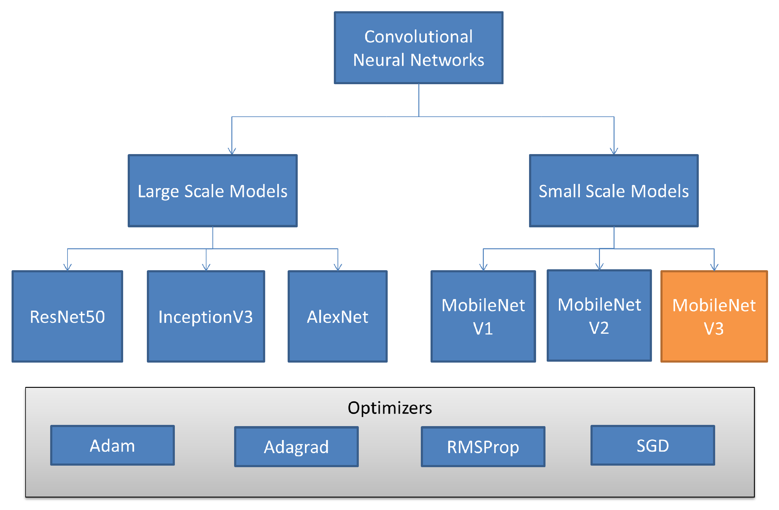
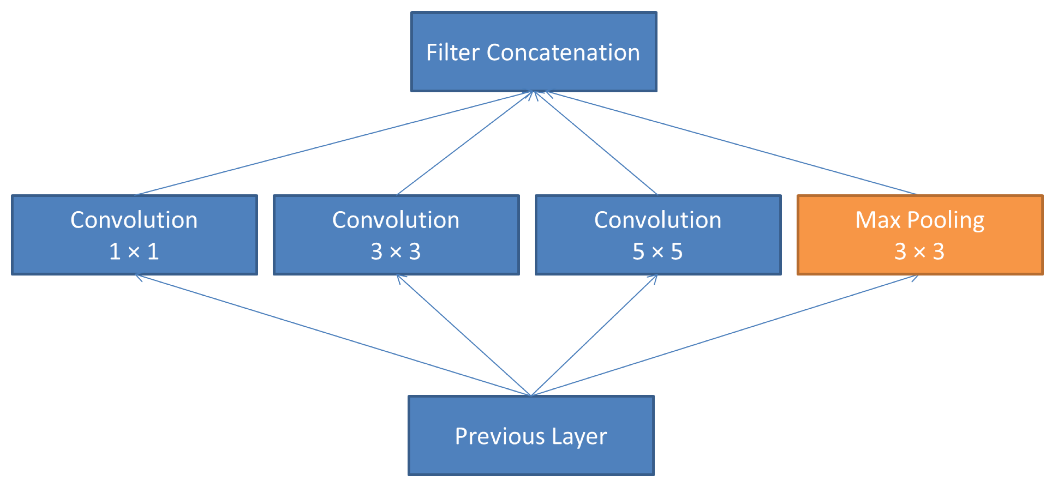
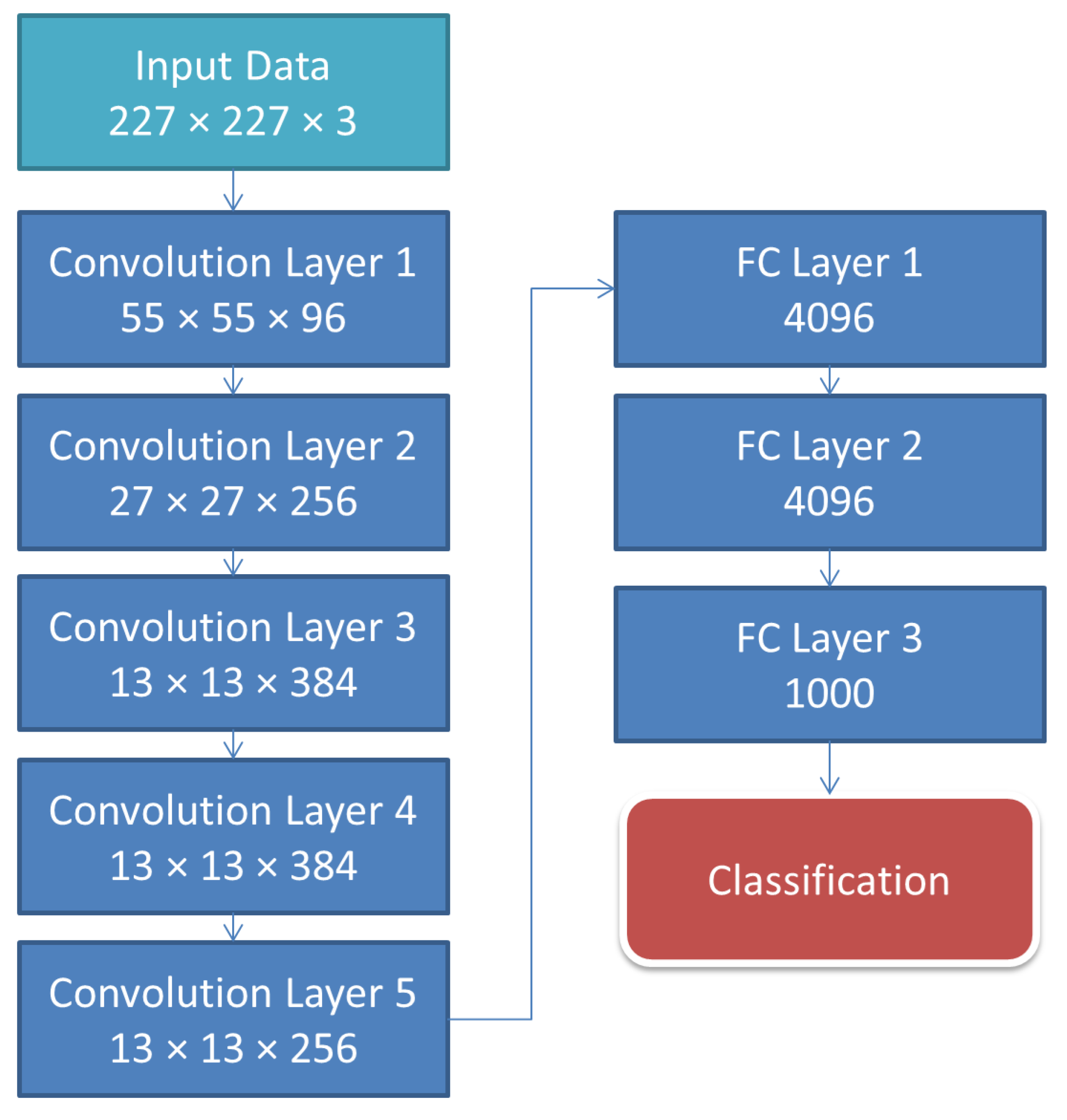
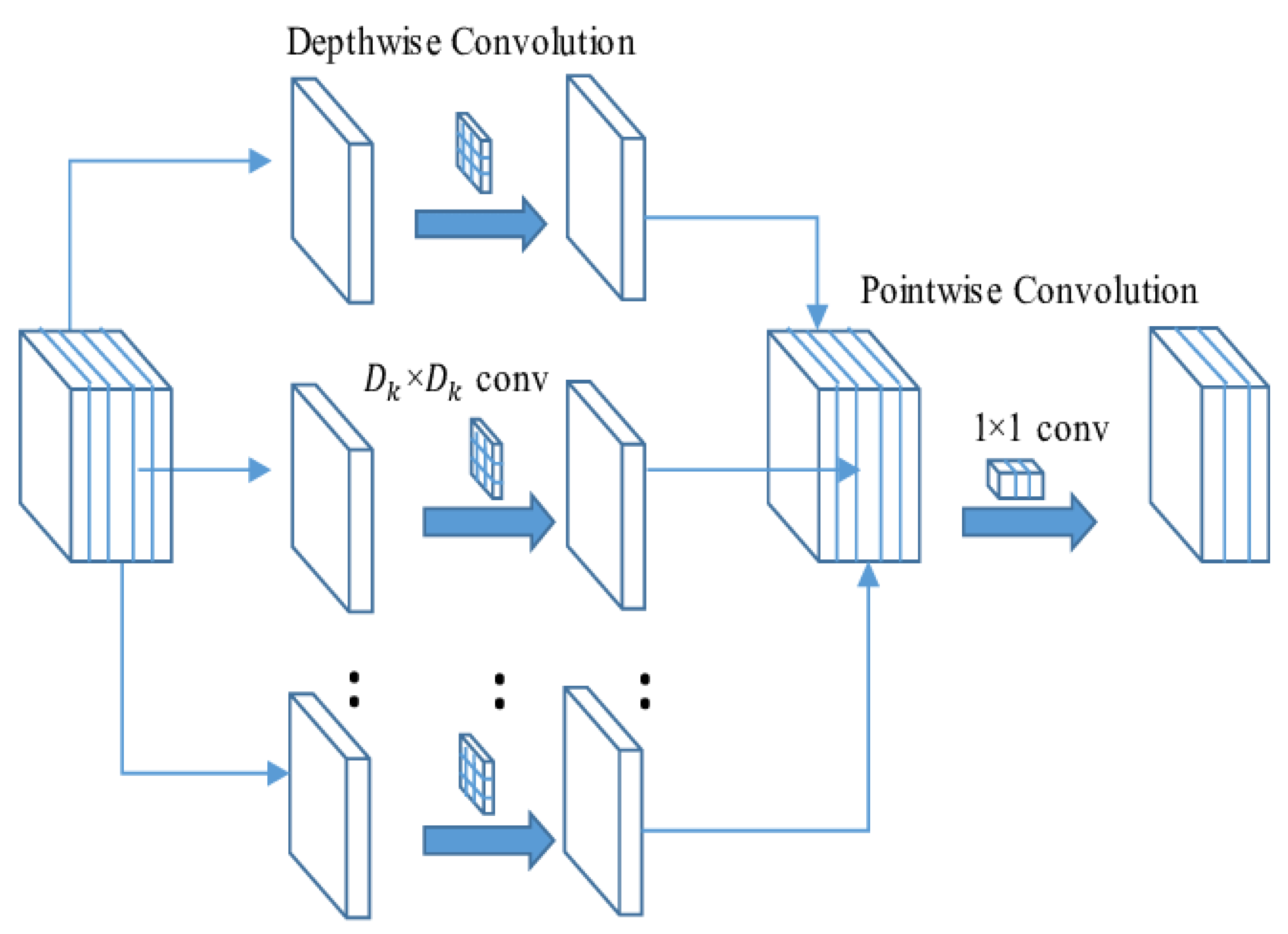
This research studies different deep learning models such as ResNet50 [16], InceptionV3 [17], AlexNet [18], MobileNetV1 [19], MobileNetV2 [20] and finally MobileNetV3 [21]. Based on the literature review, there were multiple research points that were not clear. First, the testing and deployment of MobileNetV3 on the tomato leaf diseases dataset. Second, most researches did not discuss in detail the effect of using different optimizing techniques on the previously mentioned CNN models. Third, the details of the hardware deployment of the previous models were not disclosed. In this study, a workstation and a Raspberry Pi 4 were used to test the performance of several deep learning models especially MobileNetV3 which to the best of our knowledge was not tested with PlantVillage’s tomato leaf disease dataset. Each of the CNN models were tested using different optimizers to achieve the highest possible accuracy. The Raspberry Pi 4 was chosen for the models deployment due to its low cost and due to the absence of internet connection in most of Egypt’s agricultural lands which are placed in rural areas.

This paper is divided into six sections. Section 2 consists of a description of Deep Learning, Transfer Learning and the presentation of the dataset used in this research. Section 3 is concerned with the evaluation and benchmark of different CNN models with the accuracy and loss metrics. In Section 4, the CNN models were deployed and tested on a workstation and a Raspberry Pi 4 Model B (Sony factory, Wales, UK) to evaluate their performance in real-time prediction. In Section 5, the results based on the training and deployment of the models on both the workstation and the Raspberry Pi 4 are discussed and compared. Section 6 concludes the summarized results of the implementation of different models on a Raspberry Pi as a first step in this research to build a handheld device capable of detecting tomato leaf diseases.

2. Materials and Methods

2.1. Confusion Matrix

A confusion matrix is one of the techniques used in the field of machine learning and deep learning to calculate the accuracy of classification numerically [22]. The confusion matrix has two axis which are the true and predicted label of each class, to elaborate, each row represents the true class and each column represents the predicted one. In order to measure the accuracy of the model, we can use the confusion matrix to identify the number of true positive ($TP$), number of true negative ($TN$), number of false positive ($FP$) and number of false negative ($FN$). The accuracy of the model is tested using the following equation:

$$Accuracy=\frac{TP+TN}{TP+TN+FP+FN}$$

2.2. Transfer Learning

Transfer learning is an important tool in deep learning to solve the problem of small datasets or insufficient training data [23]. It is the process of transferring the weights of a CNN model that has been trained on other large datasets such as ImageNet [24]. Nowadays, a wide variety of CNN models have been introduced such a ResNet50 [16], AlexNet [18], InceptionV3 [17]. However, as much as these CNN models have been known for their performance, accuracy and their adaptivity to different datasets, they have a large number of layers and parameters which usually slow down the training and prediction operations. Newer models have been introduced to solve that problem, such as MobileNetV1 [19], MobileNetV2 [20] and MobileNetV3 [21].

In 2012, Alex Krizhevsky et al. [18] proposed a deeper model compared to previous models such as LeNet and won the ImageNet Large Scale Visual Recognition Challenge. AlexNet proved to be a breakthrough in the field of artificial intelligence and computer vision considering it is one of the first major CNN models to have used GPU (Graphics processing unit) for training and that it was deeper than its predecessors which led to better feature extraction. However, AlexNet takes more time to train to achieve a good accuracy compared with the recent CNN models. The architecture of the AlexNet CNN model is summarized in Figure 2.

Figure 2. AlexNet Architecture Based on [25].

Deep CNNs have become popular in the field of image classification. Researchers have tried to build deeper CNN models in order to improve the classification accuracy and image recognition. However, the deeper the models, the more difficult it is to train them. Kaiming He et al. [16] proposed a residual learning framework that has made the training of deep neural networks easier and faster. One of the most successful residual networks that has achieved great results on the ImageNet dataset is ResNet-50 which is summarized in Table 1. However, ResNet50 has a complex architecture which makes it hard to implement on mobile devices.

Table 1. ResNet50 Architecture.

Layer	Output	Details
conv1	112 × 112	7 × 7, 64, stride 2
conv2	56 × 56	$\left[\begin{array}{c}1\times 1,64\\ 3\times 3,64\\ 1\times 1,256\end{array}\right]$× 3
conv3	28 × 28	$\left[\begin{array}{c}1\times 1,128\\ 3\times 3,128\\ 1\times 1,512\end{array}\right]$× 4
conv4	14 × 14	$\left[\begin{array}{c}1\times 1,256\\ 3\times 3,256\\ 1\times 1,1024\end{array}\right]$× 6
conv5	7 × 7	$\left[\begin{array}{c}1\times 1,512\\ 3\times 3,512\\ 1\times 1,2024\end{array}\right]$× 3
	1 × 1	global average pooling, 1000-d fc, softmax

The Inception model negates the idea that for a CNN model to achieve good accuracy [17], the model must be deep. InceptionV3 uses factorized convolutions which reduces the number of parameters to 58 M which is still very large compared to other CNN models. It also does not require the determination of the type of filter used in the convolutional layer and that’s the key difference that the Inception model is famous for. The InceptionV3 Building Block is shown in Figure 3.

Figure 3. InceptionV3 Building Block [26].

The MobileNet models are based on depth-wise separable convolution instead of a standard convolution [19]. Standard convolution performs the channel and spatial wise computation in one step while the depth-wise separable convolution splits the process into two steps: Point-wise convolution and depth-wise convolution. The depthwise convolution applies a filter to each channel of the image input then the pointwise convolution applies a 1 × 1 convolution to combine the outputs of the former layer. This leads to a drastic reduction in the computational power required and the model complexity. Figure 4 demonstrates the block of the dept-wise seperable convolution block.

Figure 4. Depthwise seperable convolution block [27].

The three versions of the MobileNet models has been improved ever since they were developed in 2017 [19]. The main purpose of the MobileNets was to implement a light CNN model on mobile devices with a reduced model size (<10 MB) and a reduced number of parameters. However, in some cases MobileNet models must be trained for a large number of epochs to achieve a good accuracy [28]. MobileNetV1 gained its popularity by using width and resolution multipliers which has led to a trade off in accuracy in order to reduce the computational latency and model size. Based on the previous concept, MobileNetV2 was introduced in 2018 [20] applying inverted residuals and linear bottlenecks which allowed for better memory efficient inference. In the attempts to better optimize the mobilenet architecture, MobileNetV3 was introduced in 2019 and it was developed by dropping complex layers and using H-swish function instead of standard ReLU to further increase the network efficiency and accuracy [21]. Figure 5 summarizes the architecture of MobileNetV3.

Figure 5. MobileNetV3 Architecture Based On [21].

Each CNN model is trained on the dataset using different optimization techniques such as Adam, Adagrad, RMSProp (Root Mean Square Propagation), SGD (Stochastic gradient descent) with momentum. The CNN models are summarized in Figure 6.

Figure 6. CNN Models Summary.

2.3. Dataset

PlantVillage dataset [29] was used for the images of the tomatoes. The dataset used contains the largest number of crops and plants in the world. The data obtained consists of 16,004 images and each image has a fixed size of 256 × 256 pixels. The images are divided into categorical classes, 1 healthy class and 9 disease classes: target spot, septoria leaf spot, two spotted spider-mite, yellow leaf curl virus, bacterial spot, leaf mold, mosaic virus, late and early blight. The images obtained from the dataset are then divided into 3 sets shown in Table 2. A sample of each class is shown in Figure 7.

Table 2. Data Distribution.

Class	Training	Validation	Testing	Total
Bacterial Spot Disease	1532	383	212	2127
Early Blight Disease	720	180	100	1000
Late Blight Disease	1375	343	190	1908
Yellowleaf Curl Virus	2311	577	320	3208
Target Spot	1011	252	140	1403
Septoria Leaf Spot	1275	318	177	1770
Two spotted spider mites	1207	301	167	1675
Mosaic Virus	268	67	37	372
Leaf Mold	685	171	95	951
Healthy	1145	286	159	1590
Total	11,529	2878	1597	16,004

Figure 7. PlantVillage dataset [29]: (a) Bacterial Spot Disease; (b) Early Blight Disease; (c) Late Blight Disease; (d) Yellowleaf Curl Virus; (e) Target Spot; (f) Two spotted spider mites; (g) Septoria Leaf Spot; (h) Mosaic Virus; (i) Leaf Mold; (j) Healthy Leaf.

• Training Set: 90% (80% Training, 20% Validation);
• Testing Set: 10%.

The amount of images is not large hence a case of over fitting might happen [30]. Overfitting is a concept in data science that refers to a case when a model learns too much details about the training set that it fails to generalize its knowledge when used on other data. In order to avoid overfitting and provide a generalization to be able to apply the model on images it had not seen or learned before, data augmentation must occur. Data augmentation is the process of increasing the amount of training data to avoid the model overfitting [31]. In this study, data enhancement is done by varying the following properties of the image:

• Orientation: The rotation is generated randomly between the angles of 0° to 360° by a step of 20°.
• Random Shifts: It may occur that objects may not always be centered within the image so to overcome this, shifting techniques are applied during the data augmentation phase.
• Scale: Generating multiple scaled version of images using zooming-in techniques.

3. Results

3.1. Experimental Setup

In this study, the results are divided into two phases: training and testing. The training and testing phase were deployed on the operating workstation which consists of an Intel Core i7-6800k CPU (Massachusetts, USA), NVIDIA GTX 1080 GPU (Hsinchu, Taiwan), 32 GB RAM and a 512 GB Samsung NVMe PCIe M2 Solid State Driver (Hwaseong, South Korea). The environment is set up using Microsoft’s Visual Studio Code and Python 3.7 (Delaware, United States) with the Tensorflow 2.0 (open-source artificial intelligence library).

In the direction of building a handheld device capable of tomato leaf disease detection, a Raspberry Pi 4 Model B was also used for evaluating and testing the models after training. It consists of Broadcom BCM2711, Quad core Cortex-A72 (ARM v8) 1.5 GHz processor (San Jose, California), 2 GB RAM and a 16 GB SD card for storage running on Raspbian 64-bit operating system (Cambridge, UK).

3.2. Evaluation and Benchmark

In order to measure the performance and accuracy of the proposed CNN models, they were compared using the metrics of accuracy and loss. Each training has been carried out for 50 epochs with a batch size of 32. The training of the following models was done using multiple optimizers such as Adam, Adagrad, RMSProp, SGD with momentum:

• InceptionV3;
• ResNet50;
• AlexNet;
• MobileNetV1;
• MobileNetV2;
• MobileNetV3 Large;
• MobileNetV3 Small.

The evaluation of the former CNN models is studied by applying different optimization techniques. The confusion matrices of the best and worst optimizers are discussed in the following section.

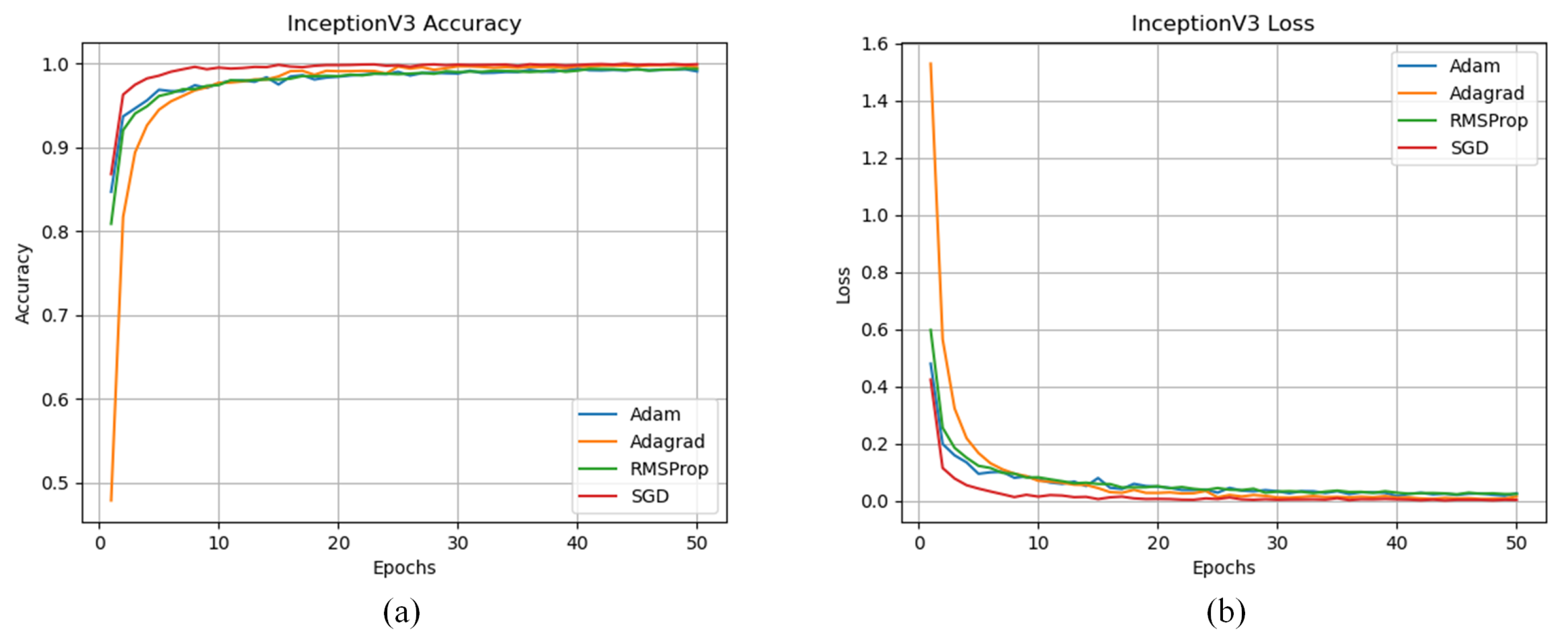
3.2.1. InceptionV3

The comparison between different optimizers used while training the dataset using the InceptionV3 CNN Model is shown in Figure 8.

Figure 8. (a) Model Accuracy, (b) Model Loss.

Based on Figure 8, it is concluded that the SGD optimizer with momentum converged in approximately 10 epochs and achieved the highest accuracy of 99.92% with a loss value of 0.0027. The Adagrad optimizer took more than 25 epochs to converge and achieved an accuracy of 99.53% with a loss value of 0.0146. The lowest accuracy was achieved by the Adam optimizer at a value of 99.06% with a loss value of 0.0255. The evaluation results of using different optimizers are summarized in Table 3.

Table 3. InceptionV3 Optimizers Evaluation.

Optimizer	Training Accuracy	Test Accuracy	Training Loss	Test Loss
Adam	99.06%	93.76%	0.0255	0.2469
Adagrad	99.53%	99.61%	0.0146	0.0097
SGD	99.92%	99.62%	0.0027	0.0110
RMSProp	99.35%	98.05%	0.0237	0.0901

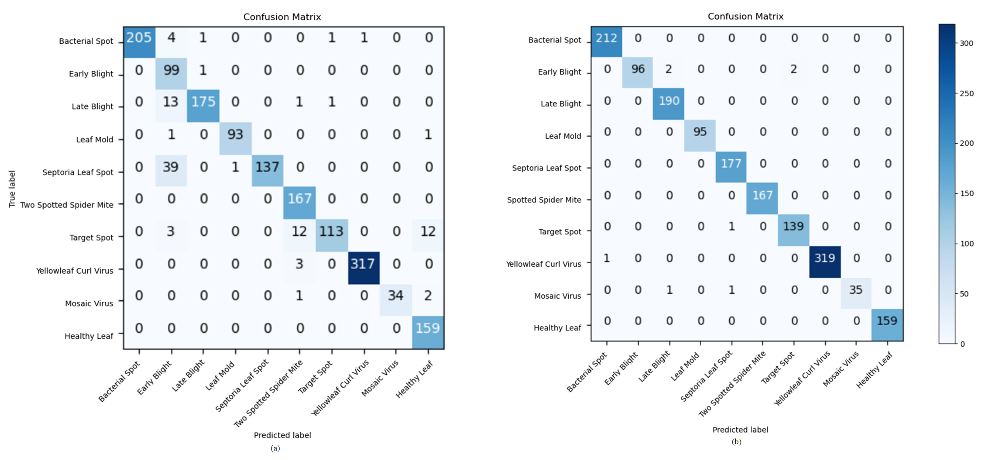
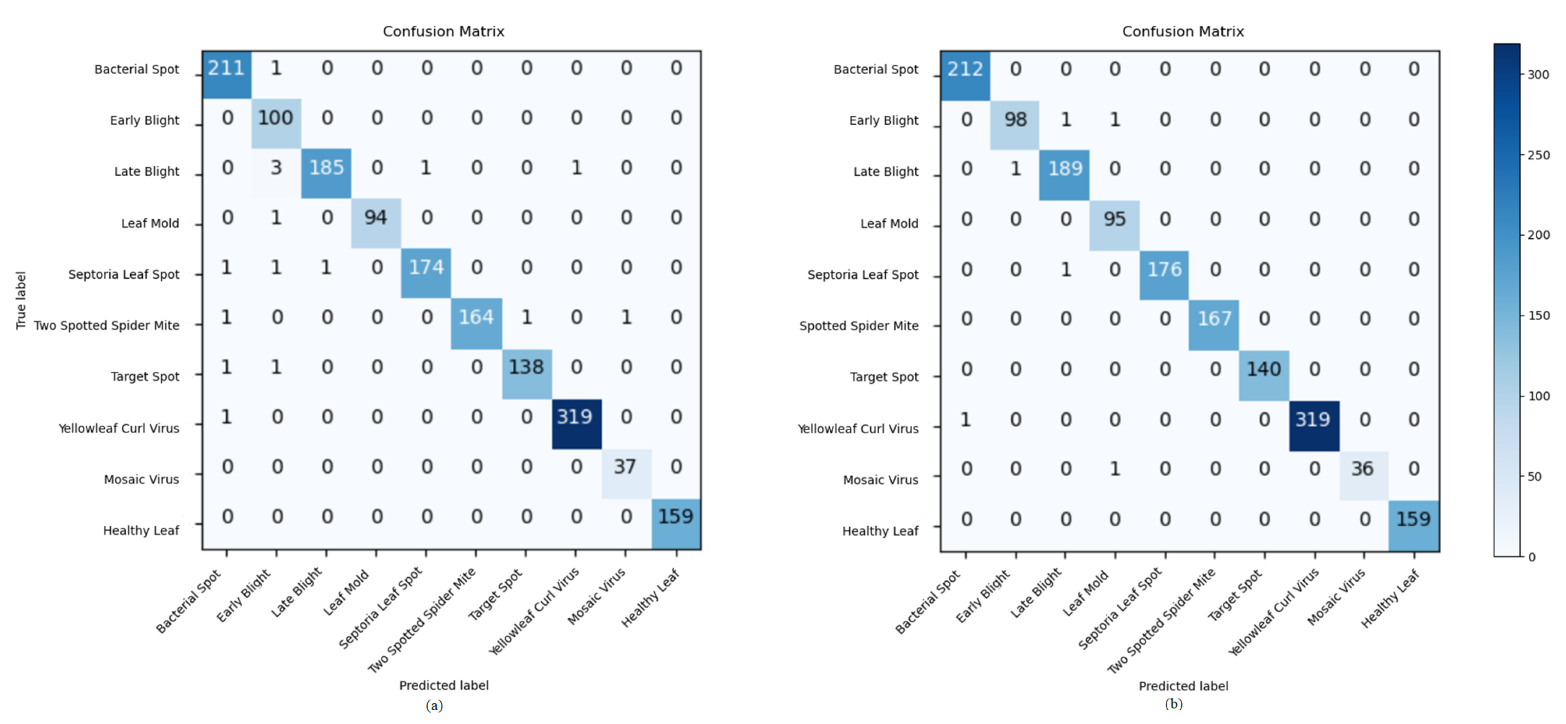
Figure 9a shows the confusion matrix for the Adam optimizer achieving the lowest accuracy of 93.76% and a loss value of 0.0901 due to a large misclassification of the Early Blight disease. Figure 9b shows the confusion matrix after testing InceptionV3 model optimized with SGD achieving the highest test accuracy of 99.62% and a loss value of 0.011.

Figure 9. (a) Adam Optimizer, (b) SGD Optimizer.

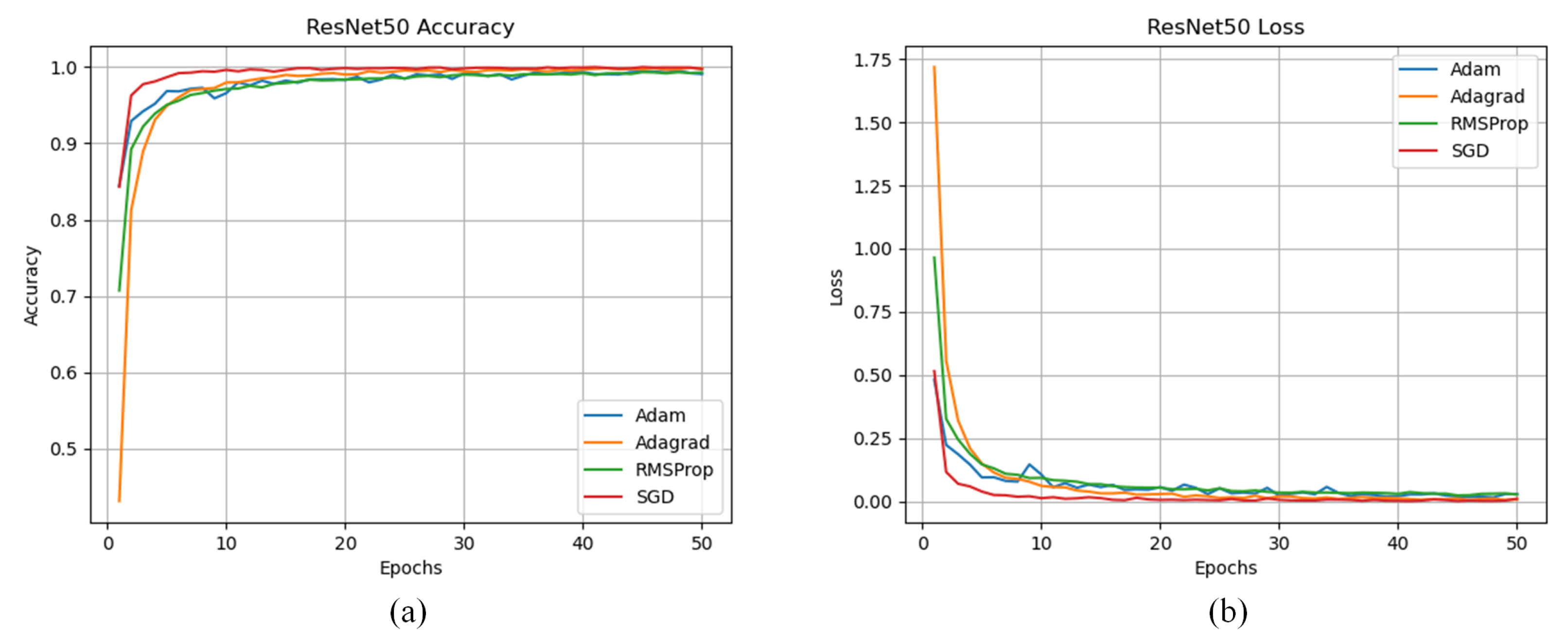
3.2.2. ResNet50

The comparison between different optimizers used while training the dataset using the ResNet50 CNN Model is shown in Figure 10. These figures demonstrates that the Adagrad optimizer converged at approximately 20 epochs and achieved the highest accuracy of 99.80% with a loss value of 0.0069 while the SGD optimizer achieved a lower accuracy of 99.74% and a loss value of 0.01 but it converged at 15 epochs. The lowest accuracy was achieved by the Adam optimizer with a value of 99.08% and a loss value of 0.0288. The evaluation results of using different optimizers are summarized Table 4.

Figure 10. (a) Model Accuracy, (b) Model Loss.

Table 4. ResNet50 Optimizers Evaluation.

Optimizer	Training Accuracy	Test Accuracy	Training Loss	Test Loss
Adam	99.08%	79.08%	0.0288	2.4515
Adagrad	99.80%	98.62%	0.0069	0.0430
SGD	99.74%	99.62%	0.0100	0.0126
RMSProp	99.28%	98.43%	0.0265	0.0565

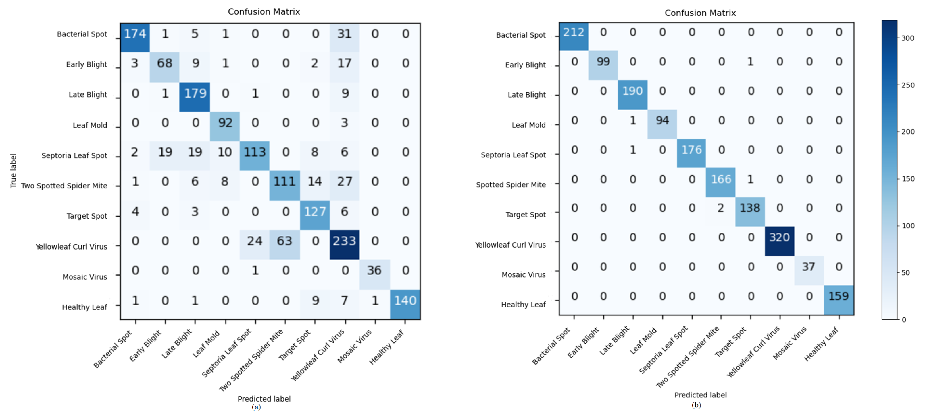
Figure 11a shows that the model trained with Adam optimizer misclassfied multiple diseases and achieved a test accuracy of 79.08% with a loss value of 2.4515. In the training phase of the model, Adagrad optimizer achieved the highest accuracy of 99.80% while the SGD optimizer achieved a marginally lower accuracy of 99.74%. However, in the testing phase of the model, SGD optimizer achieved a higher accuracy of 99.62% with a loss value of 0.0126 demonstrated in Figure 11b.

Figure 11. (a) Adam Optimizer, (b) SGD Optimizer.

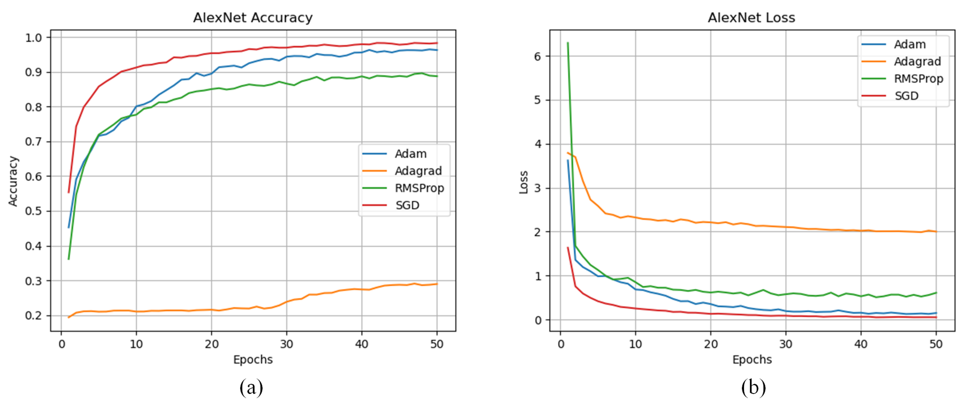
3.2.3. AlexNet

The comparison between different optimizers used while training the dataset using the AlexNet CNN Model is shown in Figure 12. Figure 12 demonstrates that Adam, Adagrad and RMSProp optimizers haven’t converged at 50 epochs and the Adagrad optimizer failed to surpass 50% accuracy. The highest accuracy was achieved by the SGD optimizer at a value of 98.26% and a loss value of 0.0520 while the lowest accuracy was achieved by the Adagrad optimizer at a value of 28.95% with a loss value of 2.0. The evaluation results of using different optimizers are summarized in Table 5.

Figure 12. (a) Model Accuracy, (b) Model Loss.

Table 5. AlexNet Optimizers Evaluation.

Optimizer	Training Accuracy	Test Accuracy	Training Loss	Test Loss
Adam	96.24%	96.18%	0.1486	0.1404
Adagrad	28.95%	34.50%	2.000	1.8941
SGD	98.26%	96.68%	0.0520	0.0957
RMSProp	88.71%	91.80%	0.6088	0.2587

Table 5 demonstrates that accuracy achieved by the AlexNet model when trained with different optimizers. The Adagrad optimizer achieved the lowest accuracy and did not converge, this is most likely due to the scaling down of the learning rate so much that the algorithm ends up stopping before reaching the optimum [32].

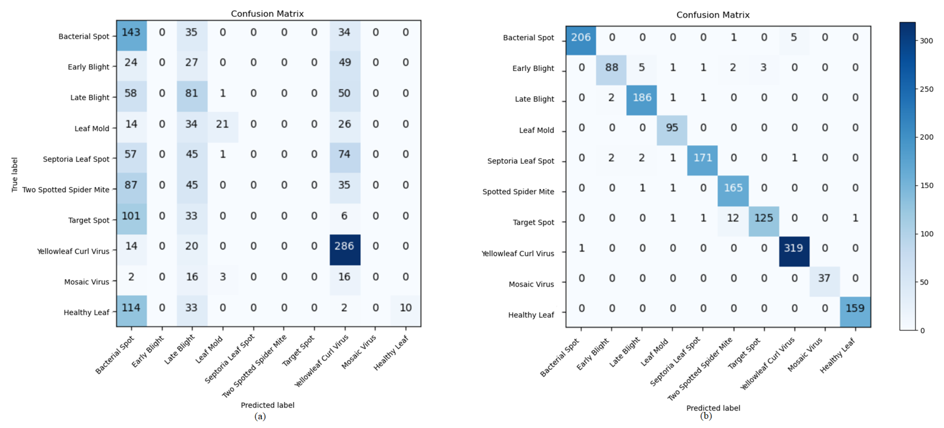
Figure 13a shows that the AlexNet model trained and optimized with Adagrad failed to converge at 50 epochs to classify tomato leaf diseases and achieved an accuracy of 34.50% with a loss value of 1.8941. The highest testing accuracy was achieved by the SGD optimizer at a value of 96.68% and a loss value of 0.0957 demonstrated in Figure 13b.

Figure 13. (a) Adagrad Optimizer, (b) SGD Optimizer.

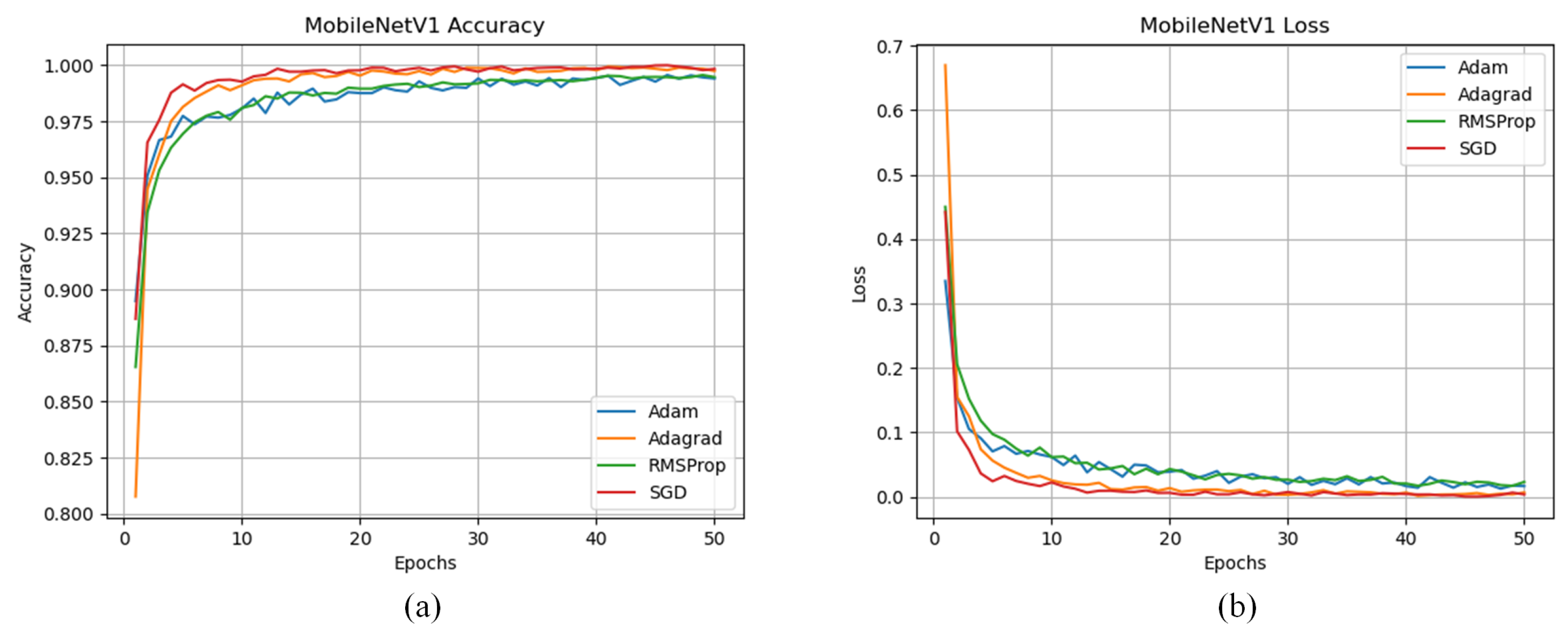
3.2.4. MobileNetV1

The comparison between different optimizers used while training the dataset using the MobileNetV1 CNN Model is shown in Figure 14. MobileNetV1 model trained with SGD converged earlier than the rest of the optimizers and achieved the highest accuracy of 99.83% and a loss value of 0.0039. The lowest accuracy was achieved by the Adam optimizer with a marginally lower accuracy of 99.46% and a loss value of 0.0811. The evaluation results of using different optimizers are summarized in Table 6.

Figure 14. (a) Model Accuracy, (b) Model Loss.

Table 6. MobileNetV1 Optimizers Evaluation.

Optimizer	Training Accuracy	Test Accuracy	Training Loss	Test Loss
Adam	99.40%	98.87%	0.0168	0.0322
Adagrad	99.74%	98.93%	0.0068	0.0343
SGD	99.83%	99.49%	0.0039	0.0130
RMSProp	99.46%	98.24%	0.0232	0.0811

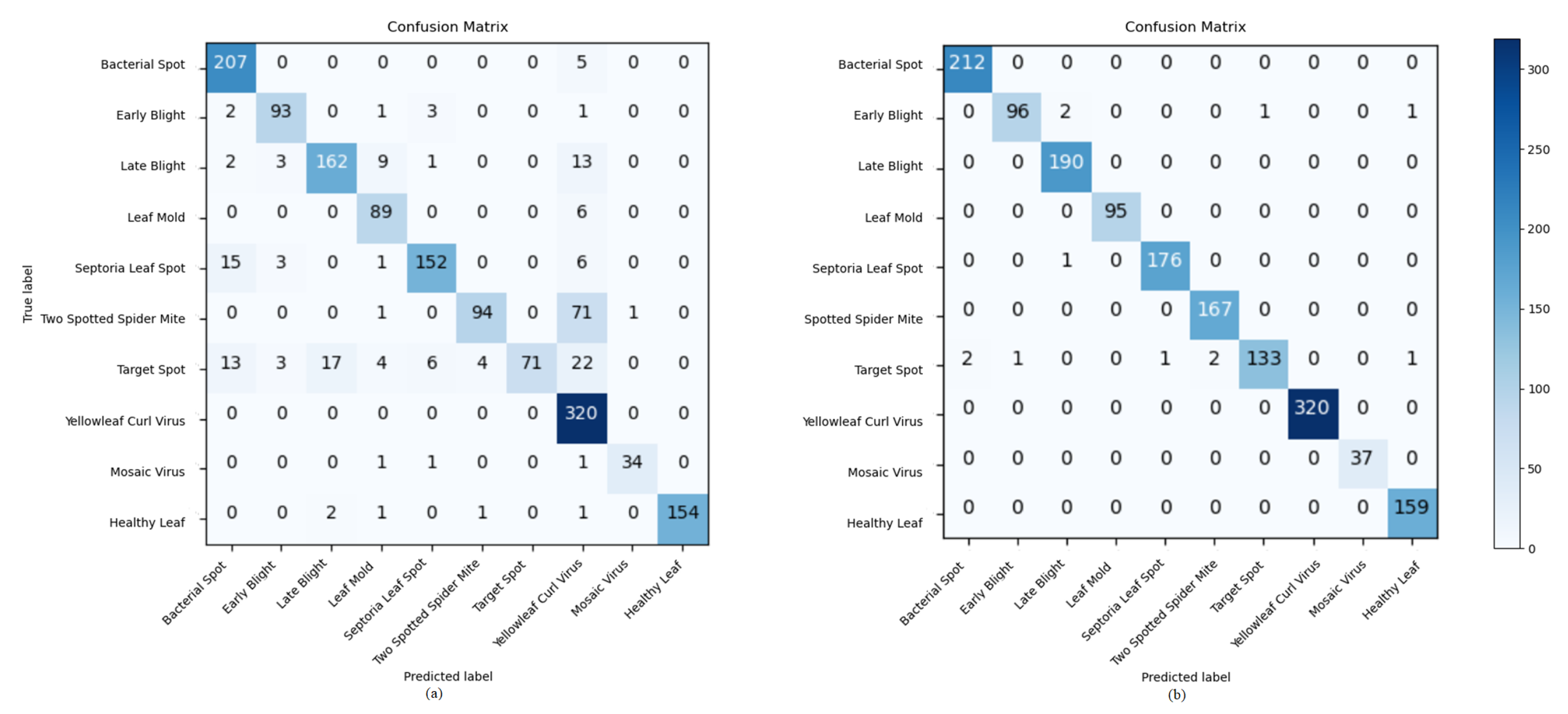
Figure 15 show the confusion matrix evaluated for the Adam and SGD optimized MobileNetV1 CNN model. Figure 15a shows that the Adam optimizer achieved the lowest test accuracy of 98.76% with a loss value of 0.0322 while Figure 15b achieved the highest test accuracy of 99.49% and a loss value of 0.0130.

Figure 15. (a) Adam Optimizer, (b) SGD Optimizer.

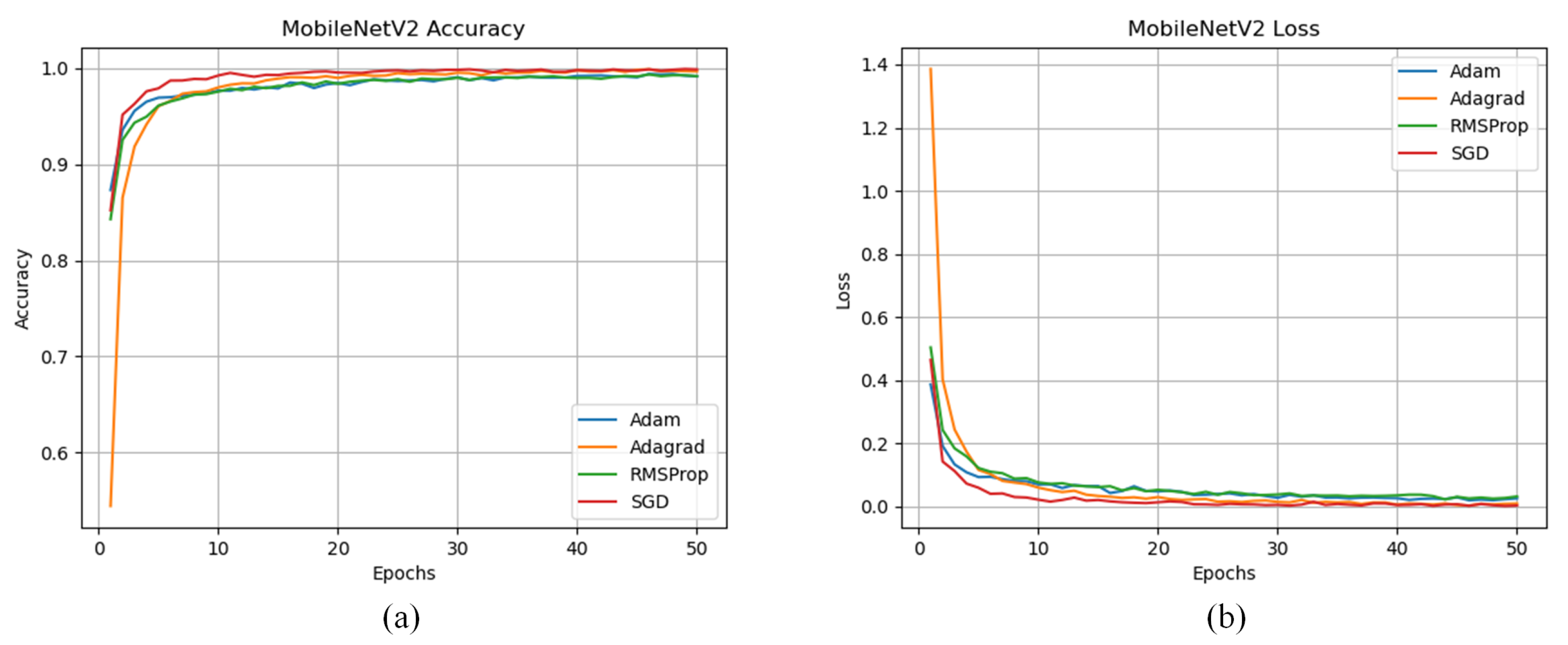
3.2.5. MobileNetV2

The comparison between different optimizers used while training the dataset using the MobileNetV2 CNN Model is shown in Figure 16. This comparison indicates that similarily to MobileNetV1, SGD optimizer achieved the highest accuracy of 99.89% and a loss value of 0.0035 and converged earlier than the rest of the optimizers. The lowest accuracy was achieved by the adam optimizer with a value of 99.17% and a loss value of 0.0262. The evaluation results of using different optimizers are summarized in Table 7.

Figure 16. (a) Model Accuracy, (b) Model Loss.

Table 7. MobileNetV2 Optimizers Evaluation.

Optimizer	Training Accuracy	Test Accuracy	Training Loss	Test Loss
Adam	99.17%	85.53%	0.0262	1.0276
Adagrad	99.68%	98.93%	0.0100	0.0379
SGD	99.89%	98.93%	0.0035	0.0351
RMSProp	99.19%	92.86%	0.0323	0.6407

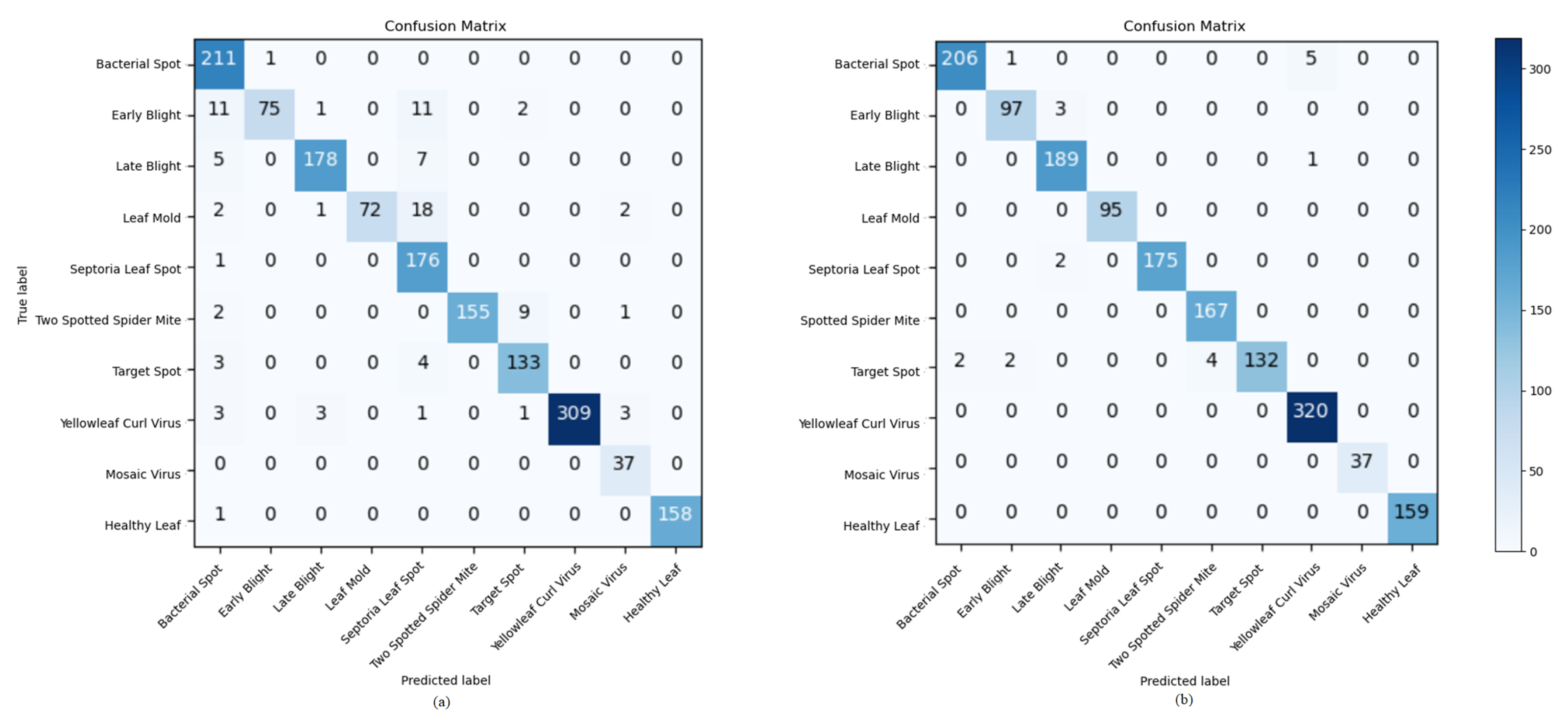
Figure 17 shows the confusion matrix evaluated for the Adam and SGD optimizers for the MobileNetV2 CNN model. Figure 17a demonstrates that the model optimized by Adam misclassified multiple diseases, hence achieving the lowest test accuracy with a value of 85.53% and a loss value of 1.0276. Figure 17b shows the confusion matrix for the SGD optimizer and it can be concluded that it achieved the highest test accuracy of 99.49% and a loss value of 0.0130.

Figure 17. (a) Adam Optimizer, (b) SGD Optimizer.

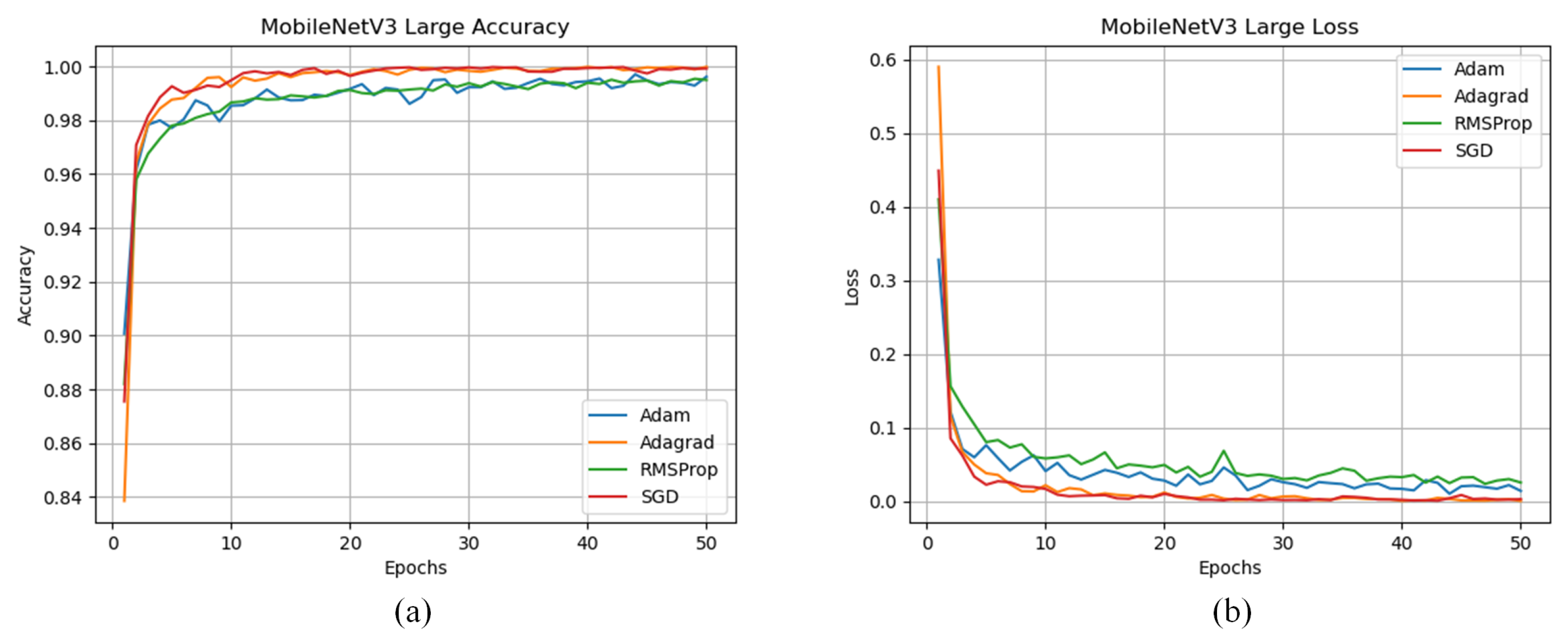
3.2.6. MobileNetV3 Large

The comparison between different optimizers used while training the dataset using the MobileNetV3 Large CNN Model is shown in Figure 18.

Figure 18. (a) Model Accuracy, (b) Model Loss.

Figure 18 demonstrates that the model optimized with SGD converged earlier than the other optimizers and achieved an accuracy of 99.92% and a loss value of 0.0029. However, the Adagrad optimizer achieved a marginally higher accuracy of 99.98% and a lower loss of 0.005. The lowest accuracy was achieved by the RMSProp optimizer at a value of 99.49%. The evaluation results of using different optimizers are summarized in Table 8.

Table 8. MobileNetV3 Large Optimizers Evaluation.

Optimizer	Training Accuracy	Test Accuracy	Training Loss	Test Loss
Adam	99.61%	94.11%	0.0141	0.2754
Adagrad	99.98%	99.81%	0.0005	0.0088
SGD	99.92%	95.67%	0.0029	0.1629
RMSProp	99.49%	92.67%	0.0254	1.0530

Figure 19 shows the confusion matrix evaluated for the Adagrad and RMSProp optimizers. Even though all optimizers had similar training accuracy, in the testing phase Figure 19b demonstrates that the Adagrad optimizer has achieved the highest test accuracy by far with a value of 99.81% and a loss value of 0.0088. The lowest test accuracy was achieved by the RMSProp optimizer at a value of 92.67% and it can be shown in Figure 19a.

Figure 19. (a) RMSProp Optimizer, (b) Adagrad Optimize.

3.2.7. MobileNetV3 Small

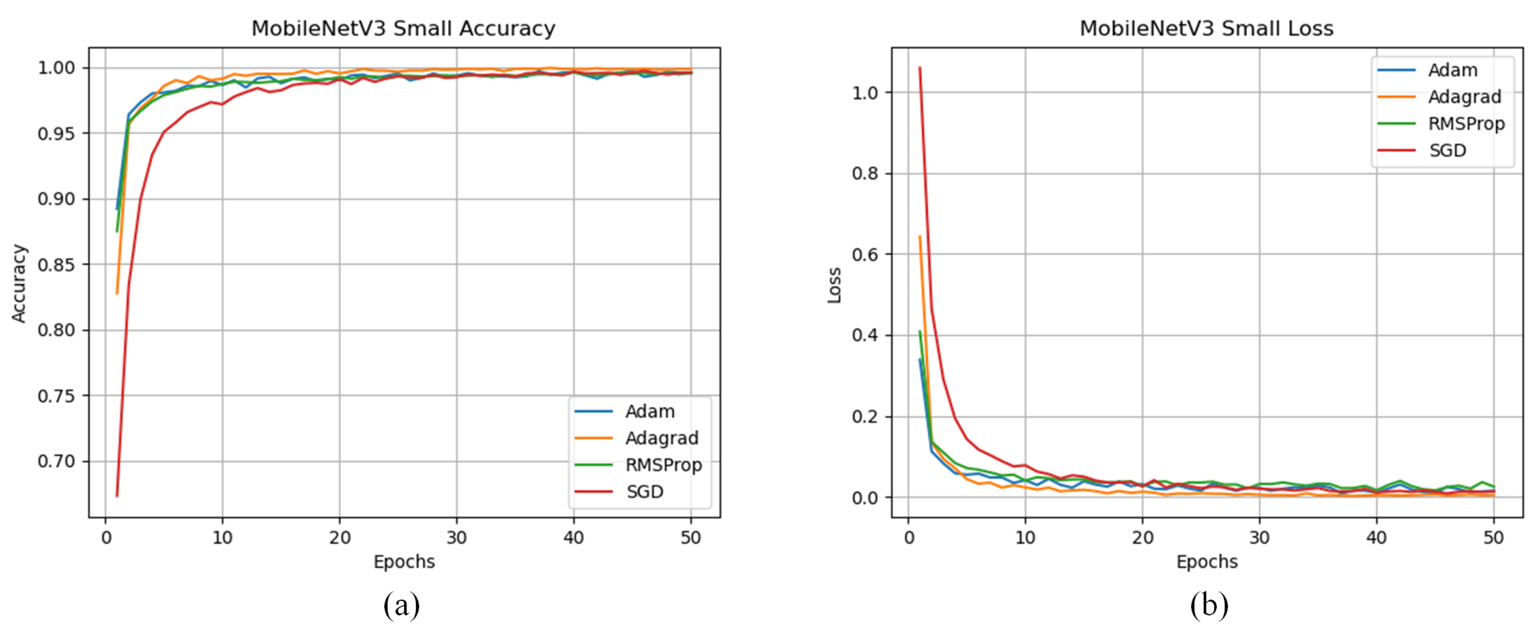
The comparison between different optimizers used while training the dataset using the MobileNetV3 Small CNN Model is shown in Figure 20. Unlike all previous results, SGD took the longest time to converge and achieved an accuracy of 99.59% while Adagrad optimizer converged earlier than the other optimizers and achieved the highest accuracy of 99.86% and a loss value of 0.0039. The evaluation results of using different optimizers are obtained in Table 9.

Figure 20. (a) Model Accuracy, (b) Model Loss.

Table 9. MobileNetV3 Small Optimizers Evaluation.

Optimizer	Training Accuracy	Test Accuracy	Training Loss	Test Loss
Adam	99.56%	98.12%	0.0149	0.0569
Adagrad	99.86%	98.99%	0.0039	0.0331
SGD	99.59%	98.30%	0.0131	0.0457
RMSProp	99.60%	94.11%	0.0246	0.9751

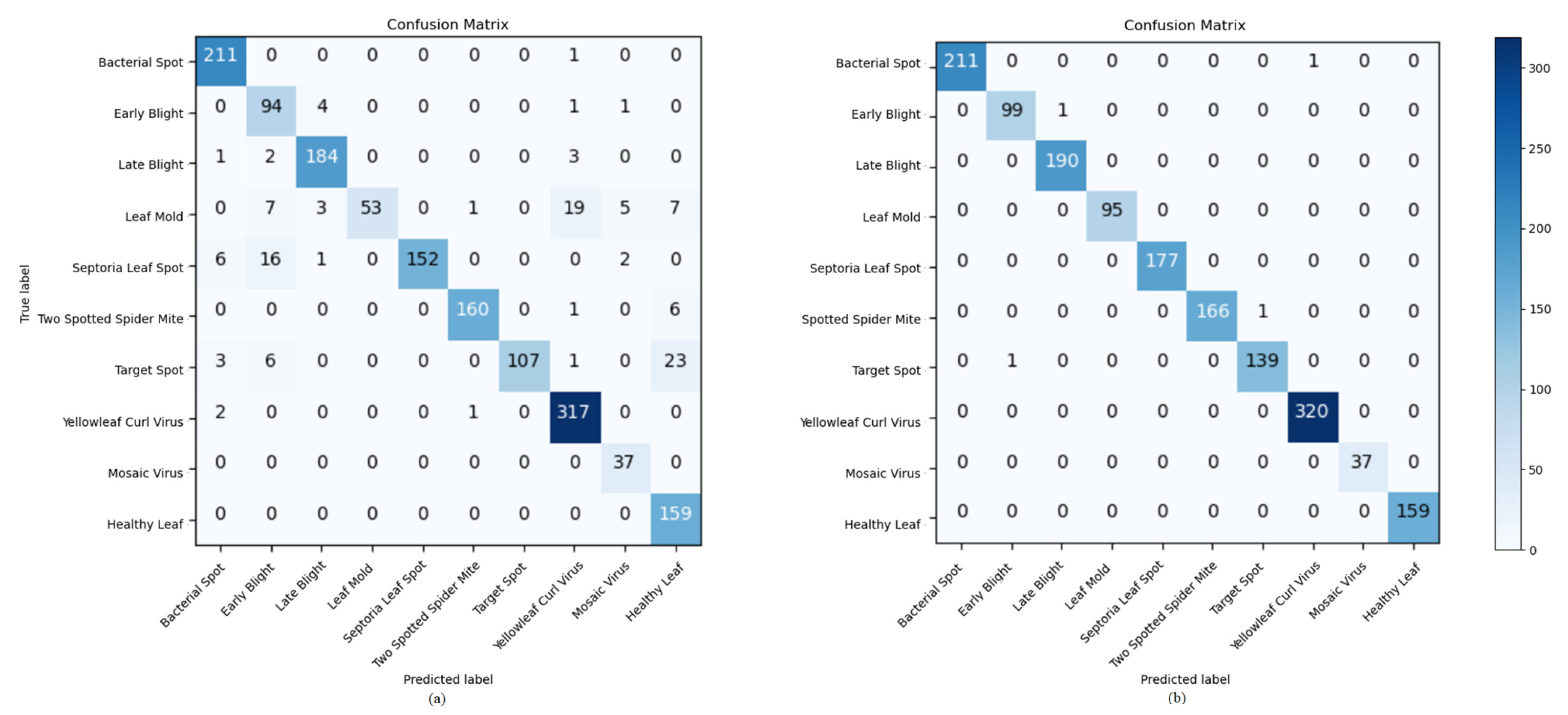
Figure 21 shows the confusion matrix evaluated for the Adagrad and RMSProp optimizers. Figure 21b demonstrates that the Adagrad optimizer had the best performance achieving a test accuracy of 98.99% and a loss value of 0.0331 while the RMSProp achieved the lowest accuracy of 94.11% and a loss value of 0.9751 leading to a large misclassifcation of diseases demonstrated in Figure 21a.

Figure 21. (a) RMSProp Optimizer, (b) Adagrad Optimizer.

4. Hardware Deployment

The previous CNN models were trained on the workstation discussed in the Materials and Methods Section. The same workstation was used to test and evaluate the performance of these models. A Raspberry Pi 4 Model B was also used to test and evaluate the CNN models’ performance on a less powerful hardware environment. The Raspberry Pi 4 Model B was chosen due to its powerful computing capability compared to its size [33] and compact design. It is the first step in this research to create a handheld device capable of real-time tomato leaf disease detection. The trained models discussed in the previous section were then transferred to the device to measure the time it takes to predict a single image. 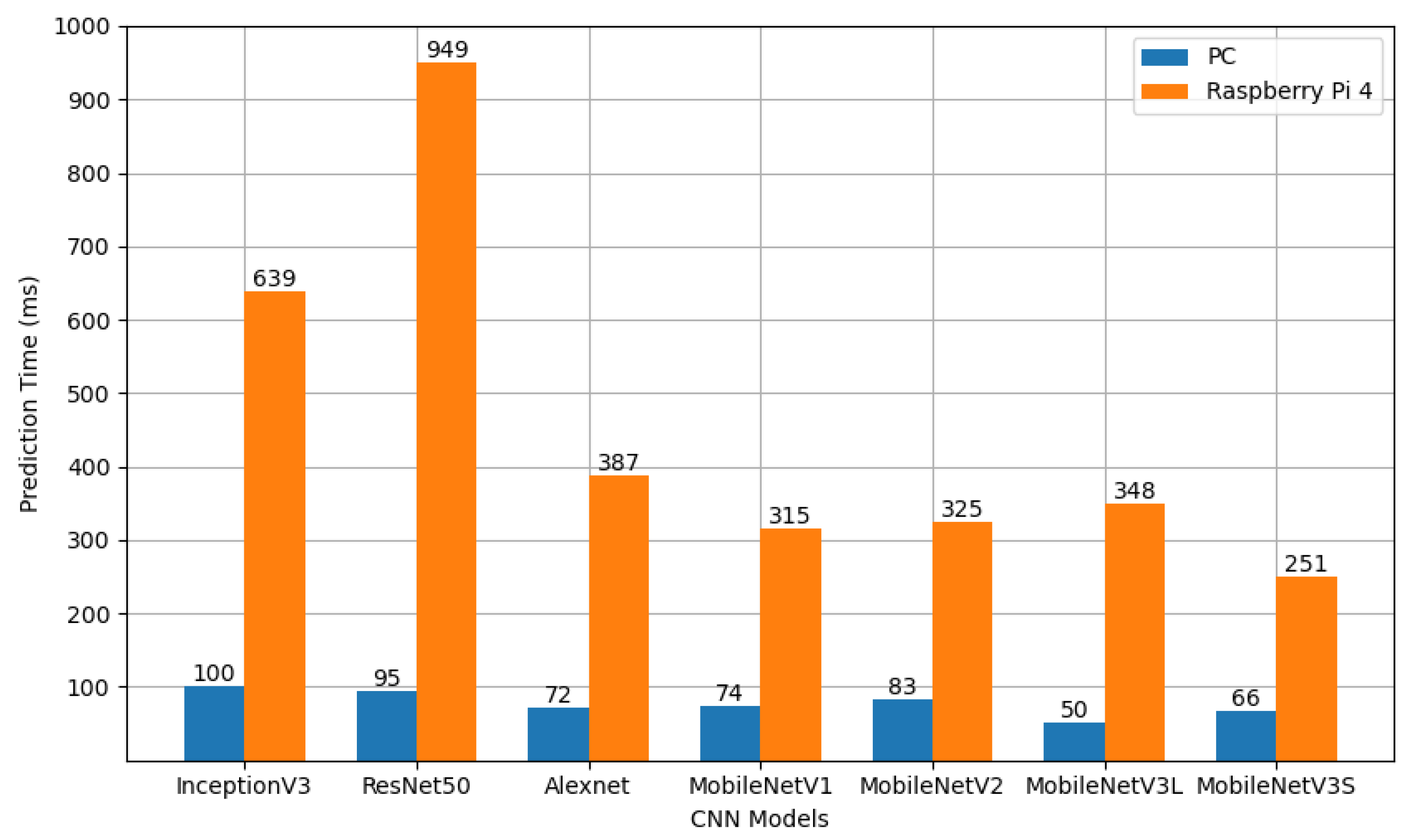Figure 22 compares the prediction time for each CNN model taken to identify a single image on the workstation. MobileNetV3 Large was able to make a prediction in half of the time it took InceptionV3 and with a marginal difference in the accuracy between the models with a value of 50 ms.

Figure 22. Prediction Time Comparison.

Based on Figure 22, MobileNetV3 Small achieved the minimum latency out of all the tested models on the Raspberry Pi 4. However, the ratio between the prediction time on the workstation and the Raspberry Pi 4 is not uniform and that could be due to the different architecture in their processors which requires more research.

The CNN models ResNet50 and InceptionV3 took the longest time to predict a single image and that is due to their complexity and deep architecture.AlexNet had a reasonable latency with an accuracy of 96.68%. The three versions of MobileNet have a similar latency value varying from 50 ms to 74 ms on the workstation and 315 ms to 348 ms with the exception of MobileNetV3 Small with a latency of 66 ms on the workstation and 251 ms on the raspberry pi 4 achieving an accuracy of 98.99% and a loss value of 0.0331 using the Adagrad optimizer. Both the workstation and the Raspberry Pi 4 were used to generate the confusion matrices. The generation time took 52 s on the workstation and 322 s on the Raspberry Pi 4.

5. Discussion

In this study, several CNN models pre-trained on ImageNet dataset were evaluated against the PlantVillage dataset in order to classify tomato leaf diseases. The dataset is classified into 10 different classes (Healthy, Bacterial Spot, Early Blight, Late Blight, Septoria Leaf Spot, Target Spot, Two-spotted Spider Mite, Yellowleaf Curl, Mosaic Virus, Leaf Mold). Transfer learning was applied on different CNN models such as InceptionV3, ResNet50, AlexNet, MobileNetV1, MobileNetV2, MobileNetV3 small and large with each model trained using various optimizers such as SGD with momentum, Adagrad, Adam and RMSProp.The learning rate for the Adagrad, Adam and SGD optimizers was set to 0.1. While the former learning rate has shown great performance with these optimizers, RMSProp required a lower learning rate (0.001) to stabilize. MobileNetV3 Large model achieved the highest accuracy of 99.81% and a loss of 0.0088 optimized by Adagrad. Table 10 summarize the best optimization technique suitable for each CNN models with the metric of the test accuracy.

Table 10. CNN Models Evaluation Summary.

Model	Best Optimizer	Test Accuracy	Test Loss	Size (MB)	Parameters
InceptionV3	SGD	99.62%	0.0110	86	21.82 M
ResNet50	SGD	99.62%	0.0126	92	23.6 M
AlexNet	SGD	96.68%	0.0957	227	58 M
MobileNetV1	SGD	99.49%	0.0130	13	3.23 M
MobileNetV2	SGD	98.93%	0.0379	9	2.27 M
MobileNetV3-L	Adagrad	99.81%	0.0088	34	4.23 M
MobileNetV3-S	Adagrad	98.99%	0.0331	13	1.54 M

6. Conclusions

In this research, the concept of smart agriculture is implemented by proposing a platform capable of tomato leaf disease detection. Multiple deep CNN techniques were studied to detect and identify tomato leaf diseases. The CNN models ResNet50, InceptionV3, AlexNet and the three versions of MobileNet were trained on the PlantVillage dataset. Each model was trained using different optimization techniques such as Adam, Adagrad, RMSProp and SGD with momentum. The highest accuracy achieved by MobileNetV3 Large using the Adagrad optimizer was 99.81% with a loss value of 0.0088. All the models were deployed and tested on a workstation and on a Raspberry Pi 4. MobileNetV3 Large also had the lowest prediction time on the workstation (50 ms) while MobileNetV3 Small had the lowest prediction time on the Raspberry Pi 4 (251 ms). Deploying MobileNetV3 Small on a Raspberry Pi 4 is the first step of research in order to build a handheld device based on IoT and Artificial Intelligence capable of automatic tomato leaf disease detection. In the future, sensors such as temperature, humidity and light will be used and the data collected will help support the prediction of the deep learning models.