Design of Efficient Floating-Point Convolution Module for Embedded System

Abstract

The convolutional neural network (CNN) has made great success in many fields, and is gradually being applied in edge-computing systems. Taking the limited budget of the resources in the systems into consideration, the implementation of CNNs on embedded devices is preferred. However, accompanying the increasingly complex CNNs is the huge cost of memory, which constrains its implementation on embedded devices. In this paper, we propose an efficient, pipelined convolution module based on a Brain Floating-Point (BF16) to solve this problem, which is composed of a quantization unit, a serial-to-matrix conversion unit, and a convolution operation unit. The mean error of the convolution module based on BF16 is only 0.1538%, which hardly affects the CNN inference. Additionally, when synthesized at 400 MHz, the area of the BF16 convolution module is 21.23% and 18.54% smaller than that of the INT16 and FP16 convolution modules, respectively. Furthermore, our module using the TSMC 90 nm library can run at 1 GHz by optimizing the critical path. Finally, our module was implemented on the Xilinx PYNQ-Z2 board to evaluate the performance. The experimental results show that at the frequency of 100 MHz, our module is, separately, 783.94 times and 579.35 times faster than the Cortex-M4 with FPU and Hummingbird E203, while maintaining an extremely low error rate.

1. Introduction

With the development of artificial intelligence (AI), CNNs have increasingly grabbed the attention of researchers in recent years, and a lot of breakthrough research results have been achieved in many fields, such as speech recognition [1,2], facial recognition [3,4], image classification [5,6,7], and object recognition [8,9,10]. Two trends have been critical to these results, namely, increasingly large scales of data and increasingly complex models that result in the increase of computation intensity. Therefore, many researchers adopt high-performance devices, such as central processing units (CPUs) and graphics processing units (GPUs), to realize convolution operations on real-time embedded systems. It is difficult for CPUs to take full advantage of parallel computing to meet real-time processing [11]. They are rarely used as CNN implementation platforms. While the computing performance of GPUs is fantastic, the high-power consumption hinders their usage in the embedded devices, with limited resources and power budgets [12]. Thus, many hardware designs for low-power embedded devices have been proposed to accelerate convolution operations [13,14], and the acceleration chip of CNNs has become an important development direction in this field.

However, embedded devices’ extremely limited resources and CNNs’ huge amount of parameters and computational complexity pose great challenges to the design. Therefore, it is particularly important to reduce the computing costs and the memory requirements. In [15], a method of network purning using an Optimal Brain Surgeon (OBS) was taken, which reduces the complexity of the network and solves the problem of overfitting by reducing the number of weights. However, this method is only effective for AlexNet and VGG, and the purning rate of networks with different structures is limited. Song et al. [16] used Tucker-Canonical Ployadic (Tucker-CP) decomposition to eliminate redundancy in the convolution layers. Additionally, their work uses the method of non-linear least squares to calculate the Tucker-CP decomposition. However, the method is hard to realize, due to the fact that the decomposition is very complicated, and the compression rate of large CNN models is limited. The authors of [17] quantized a network to a binarization network with binary weights, and multiplication operations were converted to addition operations during forward and backward propagation. The disadvantage of the binarization network was that the impact of binarization on the loss of accuracy was not considered. Zhang et al. [18] selected the optimal quantization accuracy by analyzing the value range of the parameters, which significantly improves the operation speed. Additionally, they proposed the corresponding operation units. However, the data buffer unit is not discussed in this study.

In this paper, we propose a hardware architecture for a BF16 convolution module in the form of deep pipelines to increase the computational throughput by combining quantizing network parameters with optimizing convolution operation.

This paper makes the following major contributions:

• The principle of convolution operation and the BF16 format are studied, then a dedicated FP32-to-BF16 quantization unit is proposed according to the minimum error quantization algorithm. While maintaining the accuracy of the results, the demand for memory and bandwidth is reduced;
• An efficient serial-to-matrix conversion unit and a $3\times 3$ BF16 convolution operation unit are proposed. In order to make the convolution module run at a high frequency, we optimize the critical path by eliminating the overflow and underflow handling logic cells and optimizing the mantissa multiplication.
• An analysis of data error distribution of different data formats is perfomed (e.g., INT8, INT16, FP16 and BF16);
• A $3\times 3$ BF16 convolution module using the TSMC 90 nm library is synthesized to evaluate its area consumption, and implemented on the Xilinx PYNQ-Z2 FPGA board to evaluate its performance.

The structure of this paper is organized as follows. Both the related work and the background are given in Section 2. Section 3 describes the proposed techniques for designing an efficient convolution module based on BF16. Section 4 shows the experiments and results of our work. Finally, our work is concluded in Section 5.

2. Related Work and Background

2.1. Related Work

There are many studies on accelerating CNNs on embedded devices. In [19], a new convolution architecture is proposed to reduce memory accesses, where each convolution kernel row and feature map row are horizontally and diagonally reused, respectively, and each row of partial sums is vertically accumulated. However, the construction of the Processing Element (PE) array is related to the size of the feature map rather than that of the weight, which results in the very large width of the PE array. The authors of [20] proposed a new convolution unit (CV) which was efficiently optimized by internal scheduling to avoid idleness among the CV components. However, they did not optimize the input buffer in the aspects of bandwidth. In [21], the input feature maps and the weights were stored in BRAM, and the weights were reused. However, the input feature maps were not reused, which resulted in the low memory utilization rate. To summarize, although many different methods have been proposed to accelerate CNNs on embedded devices, there are still many improvements that need to be made.

In this paper, a FP32-to-BF16 quantization unit is proposed to halve the memory and bandwidth requirements. In addition, a serial-to-matrix conversion unit is proposed to further reduce the bandwidth requirements for accessing memory and reuse the input feature maps. We also propose a convolution operation unit based on BF16 that can reuse the weights by storing them in registers.

2.2. Background

2.2.1. Convolution Operation

CNNs are composed of multiple layers of operations, such as convolution, pooling, ReLu, local response normalization, fully connected computation, and softmax [22], where the convolution layers are the key layers of the CNNs. Convolution operations are inspired by biological processes [23] in that the connectivity pattern between neurons resembles the organization of the human visual cortex. In order to explain the principle of a convolution operation, a concept called feature mapping is introduced here. When the human recognizes an image through their eyes, neighbour pixels—that is, neurons—are similar, and can form a feature area of the image. An image usually contains multiple feature areas, and these feature areas may overlap. In the CNNs, the neurons are tiled in a two-dimensional space to form a neuron plane, and the neuron plane corresponding to a certain feature area is the feature map. The mathematical nature of the feature map is a matrix.

As shown in Figure 1, the input feature map X is a 3D matrix with $N\times H\times W$, where N is the number of channels of the input feature map, and H and W are, separately, the height and width of the input feature map. The convolution kernel K is a 4D matrix with $M\times N\times H_K\times W_K$, where M is the number of kernels, and $H_K$ and $W_K$ are the height and width of kernels, respectively. The vertical and horizontal convolution strides are $H_s$ and $W_s$, respectively. The bias is a 1D matrix, with $M\times 1$ denoted as b. The output feature map O is a $M\times H_O\times W_O$ matrix, where M is the number of channels of the output feature map, and $H_O$ and $W_O$ are, separately, the output feature map’s height and width. $H_O$ and $W_O$ can be written as,

$$H_O=\lfloor \frac{H-H_K}{H_s}\rfloor +1$$

(1)

$$W_O=\lfloor \frac{W-W_K}{W_s}\rfloor +1.$$

(2)

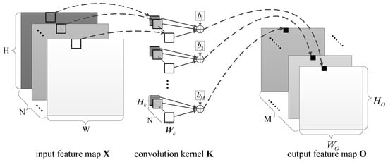
Figure 1. The illustration of convolution operation.

The pixel at $(i^{\prime },j^{\prime })$ on the mth channel of the output feature map is given as,

$$O_{i^{\prime }{j}^{\prime }}^m=\sum _{n=1}^N\sum _{i=1}^{H_K}\sum _{j=1}^{W_K}{X}_{n(i+(i^{\prime }-1)H_s)(j+(j^{\prime }-1)W_s)}^m·K_{nij}^m+b_m,$$

(3)

where $i^{\prime }\in [1,H_O]$, $j^{\prime }\in [1,W_O]$, $m\in [1,M]$.

2.2.2. BF16

BF16 is a custom 16-bit floating-point format for machine learning, which is comprised of one sign bit (S), eight exponent bits (exp), and seven mantissa bits. The value is calculated by Equation (4):

$$\mathrm{Value}={(-1)}^{\mathrm{S}}\times 2^{\exp }\times (1.\mathrm{mantissa}).$$

(4)

Figure 2 shows a diagram of the internals of three floating-point formats. BF16 is different from the industry standard IEEE 16-bit floating-point (FP16), which was not designed for deep learning applications. BF16 has three fewer bits in the mantissa than FP16, but three more in the exponent. Additionally, it has the same exponent size as FP32 [24]. Consequently, converting from FP32 to BF16 is easy—the exponent is kept the same, and the mantissa is rounded and truncated from 24 bits to 8 bits, so a small number of overflows and underflows happens in the conversion. On the other hand, when we convert from FP32 to the much narrower FP16 format, overflow and underflow can readily happen, necessitating the development of techniques for rescaling before conversion.

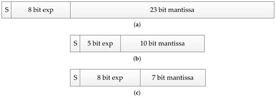
Figure 2. Data format comparison: (a) FP32: Single-precision IEEE Floating-Point Format; (b) FP16: Half-precision IEEE Floating-Point Format; (c) BF16: Brain Floating-Point Format.

Lesser precision is the drawback of BF16—essentially, three significant decimal digits versus four for FP16. Table 1 shows the unit roundoff u, smallest positive (subnormal) number xmins, smallest normalized positive number xmin, and the largest finite number xmax for the three formats. It has been well-known that the accuracy of CNN is sensitive to an exponent rather than a mantissa in a floating-point number system [25].

Table 1. A comparison of three floating-points.

Data Format	u	xmins	xmin	xmax
BF16	3.91e−03	9.18e−41	1.18e−38	3.39e+38
FP16	4.88e−04	5.96e−08	6.10e−05	6.55e+04
FP32	5.96e−08	1.40e−45	1.18e−38	3.40e+38

2.2.3. Quantization

In the CNNs, the networks can be more efficient by converting its parameters from FP32 to BF16. The reason why quantizing parameters is effective is that the trained neural networks are robust and insensitive to the noise. Therefore, by quantization, the convolution operation can be accelerated at a cost of negligible loss in accuracy, and the data-processing capability of CNNs can be improved. For the quantization, the following conclusions are drawn:

• In comparison with the FP32 networks, the speed of the convolution operation is greatly improved after quantization;
• In comparison with the FP32 networks, the memory taken up by the weights of the BF16 networks is reduced by 50%, effectively improving the data-processing capability;
• BF16 can reduce the hardware overhead while maintaining accuracy to the greatest extent.

3. The Hardware Architecture of BF16 Convolution Module

Figure 3 shows the schematic diagram of our proposed $3\times 3$ BF16 convolution module, which consists of FP32-to-BF16 quantization, serial-to-matrix conversion, and convolution operation. Each part is described as the following subsections.

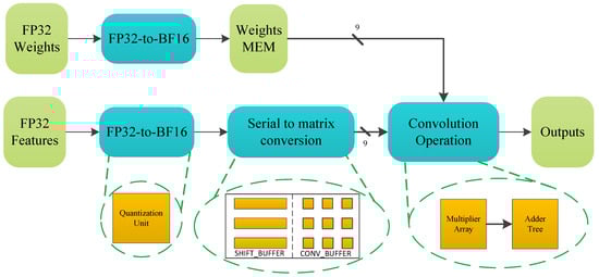
Figure 3. The schematic diagram of the proposed BF16 $3\times 3$ convolution module.

3.1. Quantization Unit: FP32 to BF16

Most of the numerical experiments conducted used simple truncation with great success when converting from FP32 to BF16 [26].

However, applying round-to-nearest-even (RNE) rounding during down-converting can result in slightly better numerical performance, such as for MobileNetV3 [27], where FP32 accuracy was fully reproduced. The RNE method works like this:

• If the absolute value of the difference between one number and its nearest integer is less than 0.5, the number is rounded to the nearest integer;
• If the difference between one number and its nearest integer is exactly 0.5, the result depends on the integer part of the number. If the integer part is even (odd), the number is rounded towards (away from) zero. In either case, the rounded number is an even integer.

The RNE operation is defined by Equation (5).

$$Round\left(x\right)=\left\{\begin{array}{c}⌊x⌋ \mathrm{if}⌊x+\frac{1}{2}⌋<x\hfill \\ ⌊x⌋ \mathrm{if}⌊x+\frac{1}{2}⌋==x \mathrm{and} ⌊x⌋ \mathrm{is} \mathrm{even}\hfill \\ ⌈x⌉ \mathrm{if}⌊x+\frac{1}{2}⌋==x \mathrm{and} ⌊x⌋ \mathrm{is} \mathrm{odd} \hfill \\ ⌈x⌉ \mathrm{if}⌊x+\frac{1}{2}⌋>x\hfill \end{array}\right.$$

(5)

As shown in Figure 4, a dedicated quantization unit is proposed to speed up this operation.

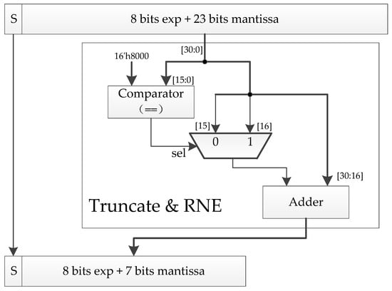
Figure 4. Our FP32-to-BF16 quantization unit.

3.2. Serial-to-Matrix Conversion Unit

In the process of inference and training of the CNNs, all convolution operations are performed in the unit matrix. According to Equation (3), it can be seen that while performing convolution operations, many matrices for convolution operations, that is, convolution matrices, are generated. According to Equations (1) and (2), it can be seen that the number of convolution matrices generated is $G=H_O{W}_O$. Consider the convolution kernel K of size $P\times P$, and define $x_{\left(i\right)}$ as the ith convolution matrix, where $i\in [1,G]$. As shown in Figure 5, the data from the second column to the Pth column of $x_{\left(1\right)}$ are the same as the data from the first column to the $(P-1)$th column of $x_{\left(2\right)}$. The matrix $x_{\left(1\right)}$ and the matrix $x_{\left(2\right)}$ have a total of $2P^2$ data, but there are $2P(P-1)$ repeated data, so the proportion of repeated data is $(P-1)/P$. The proportion of repeated data between two neighbour matrices increases with the value of P. For example, when $P=3$, the proportion of repeated data reaches 66.7%.

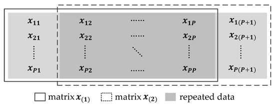
Figure 5. The illustration of a convolution matrix operation.

If all convolution matrices are calculated in parallel, too many computing resources will be consumed. Therefore, we propose a serial-to-matrix conversion unit based on the shift register to reuse the input feature maps and generate the convolution matrices in the form of pipelines, which can significantly reduce the requirements of computing resources and keep the convolution operation unit busy. As shown in Figure 6, this unit consists of CONV_BUFFER and SHIFT_BUFFER. The sizes of CONV_BUFFER and SHIFT_BUFFER are $P\times P$ and $P\times (W-P)$, respectively. Specially, the input bandwidth of this unit is very low, that is, the bit-width of the input data. The following five steps are executed in parallel in each clock cycle:

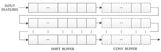
Figure 6. Our serial-to-matrix conversion unit.

• Input data from INPUT_FEATURES to the 1st row and 1st column of SHIFT_BUFFER;
• SHIFT_BUFFER performs a right-shift operation for each row;
• The data in the last column of SHIFT_BUFFER is passed onto the 1st column of CONV_BUFFER;
• CONV_BUFFER performs a right-shift operation for each row;
• The data in the last column of CONV_BUFFER are passed to the SHIFT_BUFFER of the next row.

It can be seen from the above steps that in the first $W\times P-1$ clock cycles, CONV_BUFFER has not been filled with input features, so we define $T_u=W\times P-1$ as the initialization clock cycles. In the $(T_u+1)$th clock cycle, the data stored in CONV_BUFFER is $x_{\left(1\right)}$; in the $(T_u+2)$th clock cycle, the data stored in CONV_BUFFER is $x_{\left(2\right)}$; in turn, all convolution matrices can be obtained. In particular, some invalid convolution matrices need to be eliminated through counters.

3.3. Convolution Operation Unit

Figure 7 shows our proposed $3\times 3$ convolution operation unit, which consists of BF16 multiplication and BF16 addition. In addition, for the multi-operand addition, we propose a structure of an adder tree. Each part is described as the following subsections. In particular, because a small number of overflows and underflows happens, it is not a good idea to design a circuit to handle overflows or underflows as usual. Therefore, all logic cells for overflow or underflow correction in the convolution module are removed from the critical path.

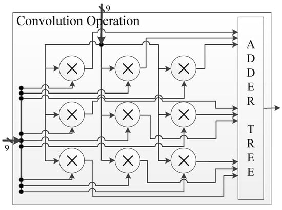
Figure 7. Our proposed convolution operation unit.

3.3.1. Multiplication Unit

The handling of 23-bit mantissa causes a large area and delay overhead in the FP32 multiplication unit implementation. However, in BF16, the use of a 7-bit mantissa saves a lot of cost in the implementation. In addition, as shown in Figure 8, we reduce the critical path delay and area overhead of the multiplier by removing the LSB 4-bit by 4-bit multiplication operation from the 8-bit by 8-bit mantissa multiplication.

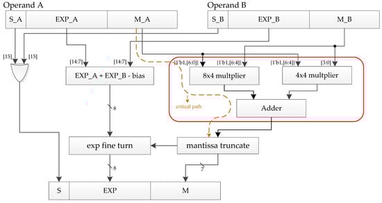
Figure 8. Our BF16 multiplication unit.

3.3.2. Addition Unit

As shown in Figure 9, the BF16 addition unit proposed in this paper is mainly composed of the following three parts: mantissa alignment, mantissa calculation, and normalization. The mantissa is self-aligned by comparing the 8-bit exponents of the two operands. The mantissa calculation method, that is, addition or subtraction, is determined according to the result calculated by XORing, the sign bits of the two operands. If the XORing result is 0, it means that operands A and B have the same signs, and two mantissas are added, otherwise two mantissas are subtracted. In particular, because the exponent and mantissa (with a hidden bit) of BF16 are both 8 bits, we use time-division multiplexing for Subtractor* to save cost in the implementation. The Leading Zeros Detector (LZD) is the most important part of the normalization. The function of the LZD is very simple. It counts the number of zeros that appear before the first “1” of the mantissa result sequence. However, it is a very complicated process to design the LZD directly according to the function description, because every bit of the output depends on all the input bits. Such a large fan-in will cause a high delay. Therefore, we propose a hierarchical 8-bit LZD (LZD8) to solve this problem, as shown in Figure 10. Its truth table is shown in Table 2.

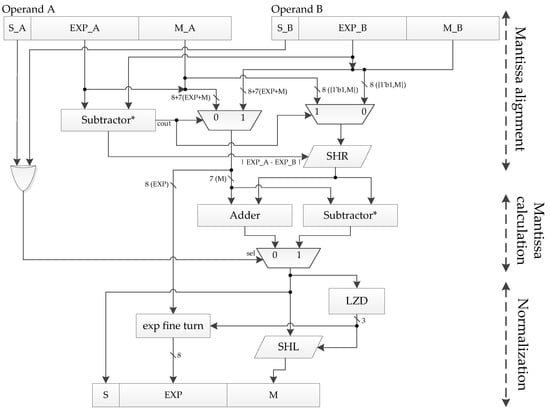
Figure 9. Our BF16 addition unit.

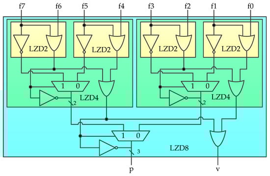
Figure 10. Our proposed hierarchical LZD8.

Table 2. The truth table of LZD8.

f [7:0]	p (3 bits)	v
1XXX XXXX	000	1 (Valid)
01XX XXXX	001	1 (Valid)
001X XXXX	010	1 (Valid)
0001 XXXX	011	1 (Valid)
0000 1XXX	100	1 (Valid)
0000 01XX	101	1 (Valid)
0000 001X	110	1 (Valid)
0000 0001	111	1 (Valid)
0000 0000	XXX	0 (Invalid)

3.3.3. Adder Tree

Consider the convolution kernel K of size $P\times P$. The result of a convolution operation can be calculated by Equation (6):

$$y=\sum _{i=1}^P\sum _{j=1}^P{x}_{ij}{w}_{ij}.$$

(6)

We can see that an operation contains $P^2$ multiplication operations and additions of $P^2$ numbers. For $P^2$ multiplication operations, $P^2$ multiplication units are used to calculate them in parallel. A classic addition tree is generally used to calculate the sum of $P^2$ numbers [28]. The classic adder tree expands the number of addends from $P^2$ to $2^{⌈{log}_2\left(P^2\right)⌉}$ by padding 0, then the sum of every two addends is passed onto the next stage as the input. In this way, the sum is accumulated step by step until y is obtained. Figure 11a shows the structure of this classic adder tree when $P=3$.

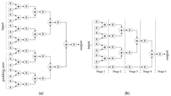
Figure 11. For a $3\times 3$ convolution operation: (a) The classic adder tree; (b) the proposed adder tree.

Although the structure of this adder tree greatly improves the parallelism of addition, it has the following two disadvantages.

First, it consumes too many hardware resources. For the additions of $\gamma$ numbers, this adder tree requires $f_1\left(\gamma \right)$ adders, $g_1\left(\gamma \right)$ registers, and $h_1\left(\gamma \right)$ clock cycles, which can be calculated by Equation (7).

$$\left\{\begin{array}{c}{f}_1\left(\gamma \right)=2^{⌊{log}_2\gamma ⌋}-1\hfill \\ g_1\left(\gamma \right)=2^{⌊{log}_2\gamma ⌋+1}-1\hfill \\ h_1\left(\gamma \right)=⌈{log}_2\gamma ⌉\hfill \end{array}\right.$$

(7)

For example, for the additions of 144 numbers ($P=12$) and 256 numbers ($P=16$), this adder tree requires 255 adders, 511 registers, and eight clock cycles. It can be seen that in the above two cases, although the number of addends is different, they consume the same number of adders, registers, and clock cycles. Obviously, this classic adder tree wastes computing resources and memory resources when the number of addends is slightly larger than $2^n$.

Second, it requires higher bandwidth. When $P=12$, the number of data which the classic adder tree needs to calculate increases from 144 to 256, and the bandwidth requirement increases by 78%.

To solve the above problems, the improvement of the adder tree proposed in this paper is as follows.

• If the number of addends is even, it can be the same as the classic adder tree;
• If the number of addends is odd, the remaining addends are passed to the next stage.

The proposed adder tree does not need additional registers to pad 0 and additional adders. However, its required clock cycles are the same as the classic adder trees. For the addition of nine numbers ($P=3$), the proposed adder tree is shown in Figure 11b.

In conclusion, as shown in Figure 11, for a $3\times 3$ convolution operation, the proposed adder tree requires eight adders, 20 registers, and five clock cycles, but the classic adder tree requires 15 adders, 31 registers, and five clock cycles.

4. Experiments and Results

4.1. Error Comparison

Using our experiment methodology, the error comparison was measured. Firstly, we generated a random feature test set with a uniform distribution between 0 and 255 to describe the input of the image. Then, we scaled the feature test set from [0, 255] to [0, 1]. In addition, we generated a random weight test set with a Gaussian distribution (mean: 0, standard deviation: 0.1), referring to the weight distribution in MobileNet-V3 [27]. Secondly, we randomly selected 500 sets of original data from the above two data sets, where each set of original data contained nine features and nine weights. Then, we used the original data (FP32) as the inputs of the convolution operation unit, and the FP32 output of the unit was used as the baseline. Finally, we quantized the original data from FP32 to INT8, INT16, FP16, and BF16, and used the quantized results as the inputs of the convolution operation unit. The outputs were compared to the baseline for error, which can be calculated by Equation (8):

$$\mathrm{error}=\frac{\left|\mathrm{quantized} \mathrm{result}-\mathrm{original} \mathrm{result}\right|}{\mathrm{original} \mathrm{result}}\times 100\%.$$

(8)

Figure 12 is a diagram of error distribution. It shows that the results obtained by convolution of fixed-point data will cause large error, where 97% of the INT8 data and 39.4% of the INT16 data have an error of more than 1%, and the mean error of INT8 is up to 12.7746%, which will seriously affect the accuracy of the network inference. However, when the original data are quantified to FP16 and BF16, it is found that 99% of the FP16 data and 86.4% of the BF16 data have error within 1%, and the mean error are 0.0078% and 0.1538%, respectively, which shows that the error caused by quantizing to a 16-bit floating-point format is much smaller than that of a fixed-point format. Moreover, as far as the floating-point format is concerned, the greater the bit width of the mantissa, the higher the accuracy, but it will also consume more hardware resources, which will be described in detail in the next subsection.

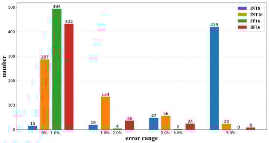
Figure 12. The diagram of error distribution.

4.2. Resource Consumption Comparison

We compared the resource consumption of our BF16 convolution module with that of FP16. For the comparison, each convolution module was synthesized by a Synopsys Design Compiler using the TSMC 90 nm library.

Table 3 shows the area of the INT16, FP16, and BF16 convolution modules and the area of their submodules at 400 MHz, 800 MHz, and 1 GHz, respectively. First, when synthesized at 400 MHz, the area of our proposed BF16 convolution module is, separately, 21.23% and 18.54% smaller than that of the INT16 and FP16 convolution modules. The one reason for this is that the quantization from a floating point to a fixed point is much more complicated than the quantization from floating-point to floating-point, so the area of the FP32-to-INT16 quantization unit is larger than that of the FP32-to-BF16 and FP32-to-FP16 quantization units. The other reason is the sizes of the adder and the multiplier are increased because the INT16 and FP16 have a larger bit-width of the mantissa stored internally in the convolution operation unit. On the other hand, as a result of the synthesis at 800 MHz, the FP16 convolution module mainly uses cells with high driving strength because the LZD11 in the FP16 addition unit is more complicated than the LZD8 in the BF16 addition unit. In addition, by optimizing the critical path to 0.89 ns, our proposed BF16 convolution module can run at up to 1 GHz, but the driving strength of the cell increased, which increased the area of the module, too. In particular, the area of our proposed 1 GHz BF16 convolution module was even smaller than that of the 400 MHz FP16 convolution module.

Table 3. Resource consumption comparison of the INT16, FP16, and BF16 convolution modules at 400 MHz, 800 MHz, and 1 GHz.

Parameters	400 MHz			800 MHz			1 GHz
	INT16	FP16	BF16	INT16	FP16	BF16	INT16	FP16	BF16
Total Area (${\mathsf{\mu }\mathrm{m}}^2$)	90,867.87	87,868.36	71,576.06	93,280.32	108,443.67	80,367.14	-	-	85,450.98
- Quantization	599.76	161.58	163.70	599.76	161.58	163.70	-	-	163.70
- Serial-to-matrix conversion	14,063.31	14,063.31	14,063.31	14,136.70	14,136.70	14,136.70	-	-	14,136.70
- Convolution operation	76,204.80	73,643.47	57,349.05	78,543.86	94,145.39	66,066.74	-	-	71,150.58

4.3. Performance Comparison

In order to complete the evaluation of performance of the BF16 convolution module, we implemented our design on FPGA. The model of the FPGA board was Xilinx PYNQ-Z2 (ZYNQ XC7Z020-1CLG400C) and the synthesizing tool was Vivado 2017.4. In addition, we used MATLAB to call the convolution function to simulate the convolution operation with FP32 on a computer with an Intel i7-8750H CPU (@3.9 GHz). The number of input neurons was 169, that is, the size of the input feature matrix was $13\times 13$. In addition, the size of the convolution kernel was $3\times 3$ and the stride was 1, that is, 121 $3\times 3$ convolution operations. The performance comparison between our design and the Reference [29] is shown in Table 4. In the Reference [29], three different experiments were conducted, where in the first and second experiments, the convolution operation was separately realized by C++ and C, and was deployed on Cortex-M4 with a floating point unit (FPU) and Hummingbird E203 processor based on the RISC-V instruction set architecture (ISA). In the third experiment of [29], the authors proposed a FP32-to-INT16 quantization unit and a cyclically callable INT16 convolution operation unit which included a $3\times 3$ multiplier array and an adder tree, then implemented them on the FPGA platform Intel Stratix IV GX EP4SGX230.

Table 4. Performance comparison of simulated convolution operations on different embedded platforms.

Parameters	Cortex-M4 [29]	E203 [29]	Stratix IV [29]	i7-8750H	Proposed
FPU (yes/no)	yes	no	no	no	no
Clock Frequency	100 MHz	100 MHz	100 MHz	3.9 GHz	100 MHz
Run Time (ms)	4.1	3.03	0.00171	0.198	0.00523
Data Format	FP32	INT32	INT16	FP32	BF16
Data Error	0%	1.28%	2.04%	0%	0.12%

As shown in Table 4, at a clock frequency of 100MHz, the convolution module proposed in this paper is 783.94 times and 579.35 times faster than the Cortex-M4 with FPU and E203, respectively. Paricularly, in comparison with the i7-8750 CPU, our module improves the convolution operation speed by 37.86 times. However, our module performs 3.06 times worse than one proposed in the third experiment of [29]. The one reason is the number of calculation cycles of BF16 is more than that of INT16. However, the data error of BF16 is 1.92% lower than that of INT16. The other reason is our convolution module includes a serial-to-matrix conversion unit, which requires additional initialization cycles. In conclusion, these comparison results clearly demonstrate that our design can effectively improve the performance of convolution operation while maintaining data accuracy.

5. Conclusions

In this paper, an efficient hardware architecture for convolution operations was proposed for resource-limited embedded devices. First, a new data format for convolution operations, BF16, was proposed to reduce the memory and bandwidth requirements with extremely low error (0.1538%) that had almost no effect on the inference of the CNNs. We further proposed hardware architecture of a convolution module based on BF16. In this architecture, a quantization unit, a serial-to-matrix conversion unit, and a $3\times 3$ convolution operation unit were proposed for CNN inference acceleration. As a result, when synthesized at 400 MHz, comparing with the area of the INT16 and BF16 convolution module, that of the BF16 convolution module was reduced by up to 21.23% and 18.54%, respectively. In addition, our BF16 convolution module can run at up to 1GHz by eliminating the overflow and underflow handling logic cells and optimizing the mantissa multiplication. We implemented the module on a Xilinx PYNQ-Z2 FPGA board. The experimental result shows that it only takes 0.00523 ms for our module to calculate 121 $3\times 3$ convolution operations while maintaining the extremely low error rate, which is superior to previous designs. In one word, our BF16 convolution module can effectively accelerate the convolution operations. In future work, we will carry on the research deeply and transplant the module into the RISC-V processor.

References

- Qayyum, A.B.A.; Arefeen, A.; Shahnaz, C. Convolutional Neural Network (CNN) Based Speech-Emotion Recognition. In Proceedings of the 2019 IEEE International Conference on Signal Processing, Information, Communication & Systems (SPICSCON), Dhaka, Bangladesh, 28–30 November 2019; pp. 122–125. [Google Scholar]
- Yang, X.; Yu, H.; Jia, L. Speech recognition of command words based on convolutional neural network. In Proceedings of the 2020 International Conference on Computer Information and Big Data Applications (CIBDA), Guiyang, China, 17–19 April 2020; pp. 465–469. [Google Scholar]
- Schroff, F.; Kalenichenko, D.; Philbin, J. Facenet: A unified embedding for face recognition and clustering. In Proceedings of the IEEE Conference on Computer Vision and Pattern Recognition, Boston, MA, USA, 7–12 June 2015; pp. 815–823. [Google Scholar]
- Chen, S.; Liu, Y.; Gao, X.; Han, Z. Mobilefacenets: Efficient cnns for accurate real-time face verification on mobile devices. In Proceedings of the Chinese Conference on Biometric Recognition, Urumqi, China, 11–12 August 2018; pp. 428–438. [Google Scholar]
- Krizhevsky, A.; Sutskever, I.; Hinton, G.E. Imagenet classification with deep convolutional neural networks. Commun. ACM 2017, 60, 84–90. [Google Scholar] [CrossRef]
- Wang, F.; Jiang, M.; Qian, C.; Yang, S.; Li, C.; Zhang, H.; Wang, X.; Tang, X. Residual attention network for image classification. In Proceedings of the IEEE Conference on Computer Vision and Pattern Recognition, Honolulu, HI, USA, 21–26 July 2017; pp. 3156–3164. [Google Scholar]
- Wang, K.; Zhang, D.; Li, Y.; Zhang, R.; Lin, L. Cost-effective active learning for deep image classification. IEEE Trans. Circuits Syst. Video Technol. 2016, 27, 2591–2600. [Google Scholar] [CrossRef]
- Lowe, D.G. Object recognition from local scale-invariant features. In Proceedings of the Seventh IEEE International Conference on Computer Vision, Corfu, Greece, 20–27 September 1999; pp. 1150–1157. [Google Scholar]
- Liang, M.; Hu, X. Recurrent convolutional neural network for object recognition. In Proceedings of the IEEE Conference on Computer Vision and Pattern Recognition, Boston, MA, USA, 7–12 June 2015; pp. 3367–3375. [Google Scholar]
- Maturana, D.; Scherer, S. Voxnet: A 3d convolutional neural network for real-time object recognition. In Proceedings of the 2015 IEEE/RSJ International Conference on Intelligent Robots and Systems (IROS), Hamburg, Germany, 28 September–3 October 2015; pp. 922–928. [Google Scholar]
- Chen, L.; Wei, X.; Liu, W.; Chen, H.; Chen, L. Hardware Implementation of Convolutional Neural Network-Based Remote Sensing Image Classification Method. In Proceedings of the International Conference in Communications, Signal Processing, and Systems, Dalian, China, 14–16 July 2018; pp. 140–148. [Google Scholar]
- Mohammadnia, M.R.; Shannon, L. A multi-beam Scan Mode Synthetic Aperture Radar processor suitable for satellite operation. In Proceedings of the 2016 IEEE 27th International Conference on Application-specific Systems, Architectures and Processors (ASAP), London, UK, 6–8 July 2016; pp. 83–90. [Google Scholar]
- Farabet, C.; Martini, B.; Akselrod, P.; Talay, S.; LeCun, Y.; Culurciello, E. Hardware accelerated convolutional neural networks for synthetic vision systems. In Proceedings of the 2010 IEEE International Symposium on Circuits and Systems, Paris, France, 30 May–2 June 2010; pp. 257–260. [Google Scholar]
- Peemen, M.; Setio, A.A.; Mesman, B.; Corporaal, H. Memory-centric accelerator design for convolutional neural networks. In Proceedings of the 2013 IEEE 31st International Conference on Computer Design (ICCD), Asheville, NC, USA, 6–9 October 2013; pp. 13–19. [Google Scholar]
- Hassibi, B.; Stork, D.G.; Wolff, G.J. Optimal brain surgeon and general network pruning. In Proceedings of the IEEE International Conference on Neural Networks, San Francisco, CA, USA, 28 March–1 April 1993; pp. 293–299. [Google Scholar]
- Song, D.; Zhang, P.; Li, F. Speeding Up Deep Convolutional Neural Networks Based on Tucker-CP Decomposition. In Proceedings of the 2020 5th International Conference on Machine Learning Technologies, Beijing, China, 19–21 June 2020; pp. 56–61. [Google Scholar]
- Courbariaux, M.; Bengio, Y.; David, J.P. Binaryconnect: Training deep neural networks with binary weights during propagations. Adv. Neural Inf. Process. Syst. 2015, 28, 3123–3131. [Google Scholar]
- Zhang, B.; Lai, J. Design and Implementation of a FPGA-based Accelerator for Convolutional Neural Networks (in Chinese). J. Fudan Univ. 2018, 57, 236–242. [Google Scholar]
- Chen, Y.H.; Emer, J.; Sze, V. Eyeriss: A spatial architecture for energy-efficient dataflow for convolutional neural networks. ACM Sigarch Comput. Archit. News 2016, 44, 367–379. [Google Scholar] [CrossRef]
- Bettoni, M.; Urgese, G.; Kobayashi, Y.; Macii, E.; Acquaviva, A. A convolutional neural network fully implemented on fpga for embedded platforms. In Proceedings of the 2017 New Generation of CAS (NGCAS), Genova, Italy, 1 September 2017; pp. 49–52. [Google Scholar]
- Zhang, J.; Li, J. Improving the performance of OpenCL-based FPGA accelerator for convolutional neural network. In Proceedings of the 2017 ACM/SIGDA International Symposium on Field-Programmable Gate Arrays, Monterey, CA, USA, 22–24 February 2017; pp. 25–34. [Google Scholar]
- Kala, S.; Nalesh, S. Efficient CNN Accelerator on FPGA. IETE J. Res. 2020, 66, 733–740. [Google Scholar] [CrossRef]
- Fukushima, K. Neocognitron. Scholarpedia 2007, 2, 1717. [Google Scholar] [CrossRef]
- Half Precision Arithmetic: fp16 Versus Bfloat16. Available online: https://nhigham.com/2018/12/03/half-precision-arithmetic-fp16-versus-bfloat16/ (accessed on 13 December 2020).
- Lee, H.J.; Kim, C.H.; Kim, S.W. Design of Floating-Point MAC Unit for Computing DNN Applications in PIM. In Proceedings of the 2020 International Conference on Electronics, Information, and Communication (ICEIC), Barcelona, Spain, 19–22 January 2020; pp. 1–7. [Google Scholar]
- bfloat16—Hardware Numerics Definition. Available online: https://software.intel.com/sites/default/files/managed/40/8b/bf16-hardware-numerics-definition-white-paper.pdf?source=techstories.org (accessed on 31 November 2020).
- Howard, A.; Sandler, M.; Chu, G.; Chen, L.C.; Chen, B.; Tan, M.; Wang, W.; Zhu, Y.; Pang, R.; Vasudevan, V.; et al. Searching for mobilenetv3. In Proceedings of the IEEE International Conference on Computer Vision, Seoul, Korea, 27 October–2 November 2019; pp. 1314–1324. [Google Scholar]
- Yu, Q.; Wang, C.; Ma, X.; Li, X.; Zhou, X. A deep learning prediction process accelerator based FPGA. In Proceedings of the 2015 15th IEEE/ACM International Symposium on Cluster, Cloud and Grid Computing, Shenzhen, China, 4–7 May 2015; pp. 1159–1162. [Google Scholar]
- Tang, R.; Jiao, J.; Xu, H. Design of Hardware Accelerator for Embedded Convolutional Neural Network (in Chinese). Comput. Eng. Appl. 2020, 27, 1–8. [Google Scholar]
Publisher’s Note: MDPI stays neutral with regard to jurisdictional claims in published maps and institutional affiliations. |
© 2021 by the authors. Licensee MDPI, Basel, Switzerland. This article is an open access article distributed under the terms and conditions of the Creative Commons Attribution (CC BY) license (http://creativecommons.org/licenses/by/4.0/).