Abstract
This study proposes a knowledge-based neural fuzzy controller (KNFC) for mobile robot navigation control. An effective knowledge-based cultural multi-strategy differential evolution (KCMDE) is used for adjusting the parameters of KNFC. The KNFC is applied in PIONEER 3-DX mobile robots to achieve automatic navigation and obstacle avoidance capabilities. A novel escape approach is proposed to enable robots to autonomously avoid special environments. The angle between the obstacle and robot is used and two thresholds are set to determine whether the robot entries into the special landmarks and to modify the robot behavior for avoiding dead ends. The experimental results show that the proposed KNFC based on the KCMDE algorithm has improved the learning ability and system performance by 15.59% and 79.01%, respectively, compared with the various differential evolution (DE) methods. Finally, the automatic navigation and obstacle avoidance capabilities of robots in unknown environments were verified for achieving the objective of mobile robot control.
1. Introduction
Neural fuzzy controllers have attracted considerable attention in control engineering. Neural networks and the fuzzy logic controller learning ability of human thinking and inference are combined to automatically adjust the controller parameters of neural fuzzy learning algorithms to obtain superior capacity and robot control results [1,2,3]. In neural fuzzy controller parameter learning, the back propagation algorithm [4,5] is widely used. This algorithm is based on the steepest descent technique for obtaining an error function, and it can achieve fast convergence to the optimal local optimum. Thus, the global optimal solution may not be determined.
Recently, some scholars have proposed evolutionary learning algorithms with neural fuzzy controllers to solve the problem of parameter optimization. Genetic and particle swarm optimization (PSO) algorithms are well-known algorithms that can mimic human physiological functions and simulate biological behavior, respectively [6]. Genetic and PSO algorithms exhibit a good global solution for space exploration capability; however, the best solution can fall in the local optima and the premature convergence problem still persists [7]. Many evolutionary algorithms have been increasingly researched over the past few decades, such as evolutionary programming algorithms and evolutionary strategies [8,9,10]. However, in the implementation of evolutionary algorithms, the user must not only determine its coding mode but also select the methods of setting appropriate parameters. Therefore, the aforementioned methods can involve high computation cost, a long computation time, trial and error, and numerous operator adjustments. To overcome these problems, many scholars have actively studied evolutionary algorithms of parameters and operator adaptability [11,12]. In the literature, different methods of adaptation by categorizing the parameter have been proposed [13,14]. To avoid local optimization and enhance global optimization search ability, the differential evolution (DE) algorithm is an excellent option. Storn and Price [15] proposed the DE algorithm, which is not only a direct and parallel search method but also an easy application of optimized search technology. The DE algorithm provides better results than the genetic algorithm and other traditional methods [16]. Many studies have proved its advantages, and it has been widely used in practice [17,18]. Three key parameters, namely the population size, mutation rate adjustment factor, and crossover rate, can considerably influence the DE. To successfully solve the problems of specific applications, considerable time is required to determine the most suitable evolution strategy and adjust its parameters through trial and error. Qin et al. [19] proposed the self-adaptive DE algorithm to reduce the time spent determining the most suitable strategy. In addition, Reynolds proposed a cultural algorithm (CA) [20]. This algorithm is a self-evolutionary algorithm and can retrieve relevant information from the problem field for evolution. The CA has two main parts, namely the population and belief spaces [21]. The population space consists of feasible solutions of the problem. This space could be any population-based evolutionary algorithm to be optimized. The belief space is similar to an information database that can store individual experience and indirectly allow other individuals to use this information as a learning reference. In the CA, information is shared by an individual with the entire population. In contrast to other evolutionary algorithms, an individual can only share information with its offspring in the CA. The population and belief spaces should be able to achieve information exchange through a communication protocol. This protocol consists of acceptance and influence functions. The acceptance function is a method to add the individual experience of the overall space to the belief space. The influence function is the feedback of individual information from the belief space to the population space. In some optimization problems [22,23], to capture useful information in order to evolve has proven to be very efficient and can considerably reduce costs.
In this study, a knowledge-based neural fuzzy controller (KNFC) is proposed for mobile robot navigation control. An effective knowledge-based cultural multi-strategy differential evolution (KCMDE) is used for adjusting the parameters of KNFC. The KNFC is applied in PIONEER 3-DX mobile robots to achieve automatic navigation and obstacle avoidance capabilities. A novel escape approach is proposed to enable robots to autonomously avoid special environments. The angle between the obstacle and robot is used and two thresholds are set to determine whether the robot entries into special landmarks and to modify the robot behavior for avoiding dead ends. Finally, the automatic navigation and obstacle avoidance capabilities of robots in unknown environments were verified for achieving the objective of mobile robot control. Relative to our previous published papers [24,25,26], the major contributions of this study are as follows: (1) an efficient KNFC is proposed for mobile robot navigation control, (2) the proposed KCMDE algorithm contains features of both the CA and DE strategy, and is implemented using the knowledge sources of the belief space in the CA to increase global search ability, and (3) in special environments, two thresholds are used to switch the controller mode between the wall-following mode and the general controller.
The remainder of the paper is organized as follows. Section 2 introduces the mobile robot structure and sensor signal. Details of the knowledge-based neural fuzzy controller and a knowledge-based cultural multi-strategy differential evolution (KCMDE) for adjusting the parameters of KNFC are described in Section 3. Section 4 presents an escape approach in special environments. The experimental results of mobile robot navigation control are illustrated in Section 5. Section 6 offers conclusions for this study.
2. Description of the Mobile Robot Structure and Sensor Signal
This section introduces the experiments conducted using the mobile robot PIONEER 3-DX [24,25,26] (see Figure 1). The robot includes eight front ultrasonic sensors, a battery, two differential drive wheels, and wheel encoders. The ultrasonic sensors are positioned on the left and right side, with six sensors facing forward at 20° intervals.
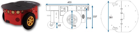
Figure 1.
Pioneer 3-DX.
In this study, the detection range of the ultrasonic sensors was approximately 20–70 cm. The configuration of the position of the ultrasonic sensors [24,25,26] is presented in Figure 2.
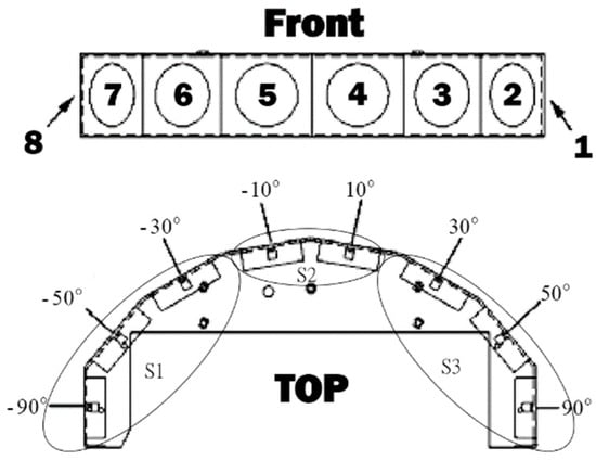
Figure 2.
Sensors of Pioneer 3-DX
The eight ultrasonic sensors (sensor1, sensor2, …, sensor8) were allocated into three call signs: S1, S2, and S3. S1 is the distance between the obstacle and left sensor of the robot, S2 is the distance between the obstacle and the front sensor of the robot, and S3 is the distance between the obstacle and right sensor of the robot. S1, S2, and S3 are depicted in Figure 2 and determined as follow:
3. The Proposed Knowledge-Based Neural Fuzzy Controller
This section describes the proposed knowledge-based neural fuzzy controller (KNFC). In this KNFC, the first three inputs of the mobile robot are the distance between the obstacle and the left front, and right sensors (S1, S2, and S3, respectively). The unit of the inputs is cm. The fourth input is the angle between the front of the mobile robot and the target (θd), and the unit is degrees. The output is the velocity of the two wheels of the mobile robot. The velocities of the left and right wheels are defined as LV and RV, respectively, and the unit is cm/s. Thus, the controller has four inputs and two outputs. The KCMDE algorithm is proposed to adjust the parameters of KNFC. The proposed KCMDE algorithm adopts the concepts of the culture algorithm (CA), which is composed of three parts, namely the belief space, population space, and information exchange protocol, comprising the acceptance and influence functions. In addition, different problems exhibit distinct performance in various DE strategies. Therefore, the KCMDE algorithm is designed using the multistrategy method. The KCMDE algorithm combines the advantages of the CA and multistrategy method to adjust the parameters of the KNFC efficiently and improve global search capability.
3.1. Structure of the Knowledge-Based Neural Fuzzy Controller
The structure of the knowledge-based neural fuzzy controller (KNFC) is illustrated in Figure 3. The KNFC implements a fuzzy if–then rule [23] in the following form:
where is the value of sensor group S1, is the value of sensor group S2, is the value of sensor group S3, is the angle between the direction of the robot and the target, Aij is the linguistic term of the precondition part, is the compensatory factor, is the left-wheel velocity of the robot (LV), is the right-wheel velocity of the robot (RV), and wj and vj are the weights of consequent parts.
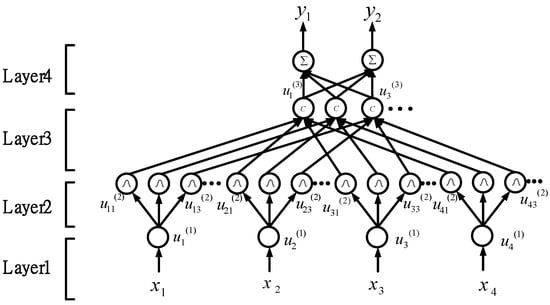
Figure 3.
Structure of the knowledge-based neural fuzzy controller (KNFC).
The operation of each node in each layer of the KNFC structure is described as follows:
- Layer 1 (input layer): Each node in this layer transfers the input value to the next layer directly.
- Layer 2 (membership function layer): Each node in this layer calculates the membership value with each value from the last layer corresponding to the linguistic of the jth rule. The operation used as the Gaussian membership function [23] is given as follows:where mij and σij are the mean and standard deviation of the Gaussian membership function, respectively, i is the ith input, and j is the jth rule.
- Layer 3 (rule layer): The nodes in this layer execute the product operation, which uses the membership values of each input corresponding to the jth rule in Layer 2. In addition, the operation uses the compensatory factor to perform if-condition matching of fuzzy rules. The compensatory operation [23] is given as follows:where is the compensatory factor and are the parameters of compensatory factors. The purpose of tuning cj and dj is to increase the adaptability of the fuzzy operator.
- Layer 4 (output layer): The nodes in this layer function as defuzzifiers. This operation summarizes the final output of the fuzzy inference as follows:
3.2. The Proposed Knowledge-Based Cultural Multi-Strategy Differential Evolution Algorithm
To realize the KNFC, a novel evolutionary learning algorithm called the knowledge-based cultural multi-strategy differential evolution (KCMDE) algorithm is proposed. The proposed KCMDE algorithm comprises the concept of the cultural knowledge source algorithm and the probability assignment of the knowledge source according to the space of the learning period. In the cultural algorithm (CA), the knowledge source is used to lead the individual to move toward the optimal solution. In cognitive science, knowledge sources can be described by the physical meaning of animals, things, and other social activities. In this study, the knowledge source was realized using the mutation strategy of the DE algorithm. Suitable individuals can gradually drive the belief space to direct the overall feasible solution in order to search a superior solution space. Next, using the method of the learning period space, the probability of each knowledge source can be adjusted instead of the traditional probability assignment. Complete suppression of certain knowledge sources can increase the adaptability of the algorithm, thereby enabling superior results to be obtained. The flowchart of the KCMDE algorithm is shown in Figure 4. The steps in the learning process of the KCMDE algorithm are described in the following text.
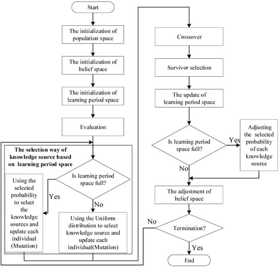
Figure 4.
Flowchart of the KCMDE algorithm.
- Step 1: Initialization of the population space
The algorithm must initialize the population space before the evolution process and achieve uniform distribution and random generation of each individual. The upper boundary and lower boundaries of each element in the individual must be predefined. Assume that xmin and xmax are the minimum and maximum boundaries of each element in each domain, respectively. The structural parameter of the KNFC is coded according to the predefined number of rules. Each individual of the population represents a KNFC. In this study, the mobile robot control problem was a four-input and two-output problem. Each input was coded into two parameters, namely mij and σij, which represent the mean of the Gaussian membership function and the variance of the Gaussian membership function, respectively. The two outputs were coded into wjand vj, where wj and vj are the weights of the consequent part of the KNFC. The other two parameters, cj and dj, are the internal parameters of γj, where γj is the compensatory factor of the KNFC. The coding method [24] is illustrated in Figure 5.
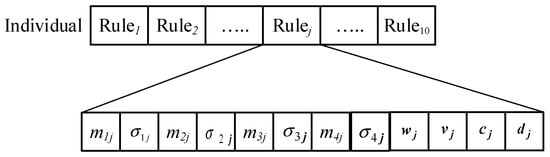
Figure 5.
Example of the coding method for an individual.
The population of the KCMDE algorithm is generated according to the coding method. The operation of each element in each individual is depicted as follows:
where xi,j represents the x th elements of the j th individual and randi(0,1) is uniformly distributed between 0 and 1.
- Step 2: Initialization of the belief space
The initialization of the belief space is empty; however, the size of the belief space is the same as the population and gradually decreases with the evolution of the generations, whereas the number of individuals that become paragons decreases over time.
- Step 3: Initialization of the learning period space
The initialization of the learning period space is empty. The learning period space is composed of successful memory and failed memory. The size of the learning period space is set according to the parameter LP (the size of the successful memory and failed memory), which is predefined by the user. In this study, the LP is set to 30. This space is responsible for recording each generation of the selected source of knowledge to improve individual performance. If the individual performance of the selected knowledge improves, the number of the selected knowledge for the successful memory increases. By contrast, the number of the selected knowledge for the failed memory increases.
- Step 4: Evaluation of each individual
Evolutionary algorithms usually rely on the performance of the individual to decide the selection progress. The larger the fitness function, the more improved are performance and fitness values. The evaluation operation is expressed as follows:
where represents the l th the real of the left-wheel and right-wheel speeds of the mobile robot, represent the l th the desired (training data) of the left-wheel and right-wheel speeds of the mobile robot, and Nt is the size of the training data.
- Step 5: Selection process of the knowledge source based on the learning period space
When the learning period space is not filled, the selection probability of each knowledge source is set as equal. Once the learning period space is filled, the selection probability of each knowledge source changes. After the learning period space is filled, the selection probability of each knowledge source is based on the roulette-wheel area. The initial roulette-wheel area is the same. Thus, selection probability is used to select the knowledge source, which is used to update the current individual. The belief space of the KCMDE algorithm has five knowledge sources, namely situational, normative, topographical, domain, and history knowledge. In this study, three knowledge sources, namely situational knowledge, topographical knowledge, and history knowledge were used. These sources are described as follows:
- 1.
- Situational knowledge
The best individual in the evolutionary process is a model to lead other individuals for situational knowledge. In this study, the differential mutation strategy DE/best/1 [16] is used, and evaluation of the initial population is necessary in initial situational knowledge. Therefore, the initial best individual is determined and stored. For situational knowledge, the mutation strategy is affected in the following way:
- 2.
- Topographical knowledge
Topographical knowledge presents spatial information to build a map of the fitness landscape in the evolution process. A tree structure was used to achieve topographical knowledge. In the tree structure, the root can only have two children that represent two differential mutation strategies, namely and . Therefore, the influence function moves the children using DE/current-to-best/1 [16] as follows:
where represents the current individual, is the best individual in the belief space, an .
- 3.
- Historical knowledge
This is the best historical knowledge of the individual’s past records as an event-based memory, such as local optimal. Therefore, historical knowledge is achieved as a list to store the w temporal on the last search. If the population diversity decreased during late evolution in this study, the best individual was used as a model to induce premature convergence. To obtain fast search but not early convergence, a new mutation strategy, namely DE/current-to-w past best [16], was implemented to use the wth best individual in a history list to guide the other individuals (Figure 6). The expression for the DE/current-to-w past best mutation strategy is as follows:
where is randomly selected as one of the wth best individuals in the belief space.
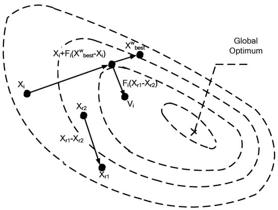
Figure 6.
The DE/current-to-w past best mutation strategy.
- Step 6: Crossover
To implement the DE operation search strategy, the KCMDE algorithm uses the crossover operation. The population after the mutation () and the population before the mutation () based on the crossover rate (CR) was used to generate the new population (). The operation of is expressed as follows:
where is the CR and defined by the user, is the dimension number of the individual, and is a uniform random number operator.
- Step 7: Survivor selection
In survivor selection, the new individual () is evaluated using Equation (16). If the performance of the new individual () is better than that of the original individual (), the new individual () is used instead of the original individual ().
- Step 8: Update of the learning period space
The update of the learning period space is based on whether the individual () of the selected knowledge source is better than the original individual () in the current generation. When the individual () of the selected knowledge source is not better than the original individual (), the failed factor (nfk,g) is increased. By contrast, the successful factor (nsk,g) is increased. The number of generations (g) is not larger than the size of the learning period space in Table 1 and Table 2. Until the learning period space is filled, the selection probability of each knowledge source is marginally adjusted. When the number of generations is larger than the size of the learning period space in Table 3 and Table 4, the earliest records stored are removed to enable new values in the current generation to be stored. When the evolution generation is increased, the selection probability of each knowledge source is adjusted.

Table 1.
g < Learning period (LP situation) of successful memory.
Table 2.
g < LP situation of failed memory.
Table 3.
g > LP situation of successful memory.
Table 4.
g > LP situation of failed memory.
In the aforementioned tables, LP is the size of the learning period space, strategy k is the kth knowledge source, nfk,g is the number of failed attempts in the g generation, and nsk,g is the number of successful attempts in the g generation.
When the learning period space is filled, execute step 9. Then, execute step 10.
- Step 9: Adjusting the selection probability of each knowledge source according to the learning period space
In the KCMDE algorithm, the selection probability of each knowledge source is adjusted according to the failed factor (nfk,g) and successful factor (nsk,g). In the initialization of KCMDE, the selection probability of each knowledge source is set as equal. The success rate (Sk,g) is operated by gathering the failed factor (nfk,g) and the successful factor (nsk,g) from 1 to LP in the learning period space. The operation is expressed as follows:
where k is the number of the knowledge source; Sk,g, which enters the generation successfully based on previous LC generation, is the success rate of the offspring individual generated by the kth strategy; and ε is the value that prevents the success rate from being equal to 0.
After the success rate of the knowledge source is generated, the proportion of each knowledge source is operated using Equation (16) and summarized to 1. Equation (16) represents the selected probability of each knowledge source and is expressed as follows:
where K is the number of knowledge source, k is the k th knowledge source, g is the evolution generation, and pk,g is the selected probability of each knowledge source.
- Step 10: Adjustment of the belief space
The belief space of the KCMDE algorithm is a space that stores the experience of the paragon individual. Irrespective of whether the individual becomes a paragon, the adjustment of the belief space is influenced. The evaluation method of acceptance is designed. The evaluation method of acceptance is responsible for evaluating which individual becomes a paragon and adjusts the belief space. The elite selection mechanism [22] is used, and the specific proportion of population in which the individual has superior fitness is selected to become the paragon. The proportion gradually decreases when the number of evolution generations increases. The operation is expressed as follows:
where n% is predefined by the user and represents the proportion of acceptance, I is the number of the population, and t is the number of the current generation.
4. An Escape Approach in Special Environments
In a complex environment, the controller is responsible for moving the mobile robot away from the obstacle and close to the target. When the mobile robot encounters special environments, such as concave, continuous concave, and V-shaped environments, the mobile robot can produce dead-end traps or infinite loops. Thus, the mobile robot cannot successfully reach the target. The escape special environment approach is designed for solving the four types of special environment (Figure 7).
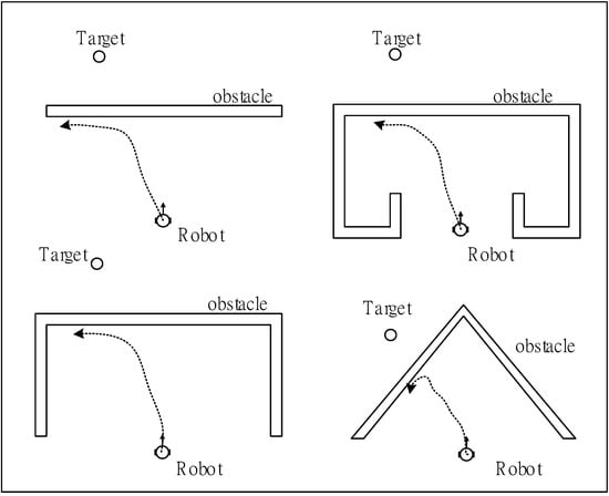
Figure 7.
Special environments.
In the design of the escape special environment approach, first, two thresholds, namely A and B, are designed. Thresholds A and B are angle values and are predefined. When the angle between the direction of the mobile robot and the target is larger than threshold A, the robot enters the wall-following mode. Threshold B is the angle when the mobile robot enters the wall-following mode. The angle between the direction of the mobile robot and the target enforces threshold B. Thus, the mobile robot enters the wall-following mode. When the angle between the direction of the mobile robot and the target is equal to threshold B again, the mode of the mobile robot is transferred back to the normal controller navigation mode. The flowchart of the escape special environment approach is illustrated in Figure 8.
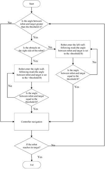
Figure 8.
Flowchart of the escape special environment approach.
The schematic of the escape special environment approach is depicted in Figure 9. First, no obstacles are present near the robot. The mobile robot moves toward the target until it encounters the obstacle (point 1), when the angle between the direction of the mobile robot and the target is larger than threshold A (point 2). At this time, the mobile robot judges to the left of the robot and no obstacle is accounted for. When the angle between the direction of the mobile robot and the target is larger than threshold B, the robot enters the wall-following mode (point 3). Thus, the mobile robot moves along the wall (point 4). When the angle between the direction of the mobile robot and the target is equal to threshold B again, the mode of the mobile robot is transferred back to the normal controller navigation mode (point 5).
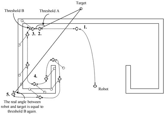
Figure 9.
Schematic of the escape special environment approach.
5. Experimental Results
The proposed KNFC based on the KCMDE algorithm was tested using the mobile robot Pioneer 3-DX to navigate in the unknown environment. The KNFC was tested in a complex and unknown environment to prove its navigation ability. The learning performance of the KCMDE algorithm was then compared with that of the DE strategy. Finally, the learned KNFC by the KCMDE algorithm were simulated in an unknown environment and the special environment. The code of our technique (as well as dataset) is made publicly available in [27].
5.1. Performance Comparison of Various DE Methods
The performance of the proposed KNFC based on KCMDE algorithm was compared with that of the DE/best/1, DE/current-to-best/1, DE/rand-to-best/1, and DE/current-to-rand/1 mutation strategies [16] of the original DE. KCMDE has four parameters: a population size PS, a crossover rate CR, a scale factor F, and a learning period space (LP). In general, the larger the PS, the more robust will be the search, with increased computational cost. However, a large CR will lead to large perturbations and a slow convergence speed. On the other hand a low CR will lead to rapid loss of diversity. Additionally, if F is small, it will lead to extensive exploitation and thus a much higher likelihood of non-convergence. On the other hand, a large value of F will lead to over exploration and a significantly reduced convergence speed. Finally, the LP will guide the search in population. If LP closes to PS that is meaningless, and LP is small, this easily makes the solution fall into the local optimum. The initial parameters of various DE were as follows: the population size was 100, CR was 0.9, scale factor was 0.5, and size of the learning period was 30 (Table 5). Each algorithm was run 30 times. The mean of the fitness of each generation of 30 runs was calculated, and these data were plotted into the convergence curve. In the DE/best/1, DE/current-to-best/1, DE/rand-to-best/1, DE/current-to-rand/1, and KCMDE algorithms, the number of fitness evaluations (FES) is 1000 (generations) × 100 (population size) = 100,000 for a fair comparison. The convergence curve is displayed in Figure 10. The convergence curve indicates that the KCMDE algorithm has the fast convergence features of DE/best/1 and the superior learning features of DE/current-to-best/1. Thus, the KCMDE algorithm, which combines the concept and multistrategy, is an effective algorithm. Table 6 indicate that the learning ability of the proposed KNFC based on the KCMDE algorithm is superior to that of other algorithms.
Table 5.
Initial parameters of knowledge-based cultural multi-strategy differential evolution (KCMDE).
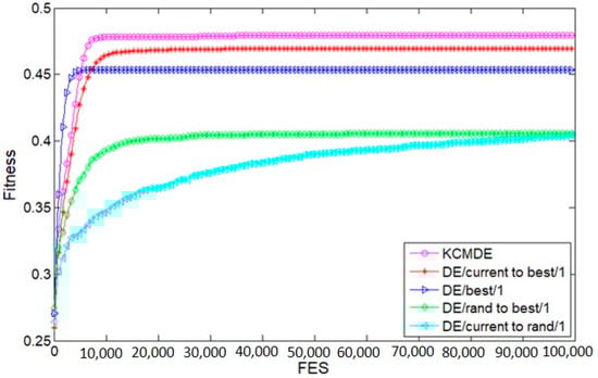
Figure 10.
Convergence curves for the various algorithms.
Table 6.
Performance comparison of the various algorithms.
5.2. Navigation Ability in Complex Environments
A map with complex obstacle environments was used to test the mobile robot navigation ability of the KCMDE algorithm and compare it to other DE/strategy algorithms. Equation (19) was designed to test the mobile robot navigation ability of the algorithms such as DE/best/1, DE/current-to-best/1, DE/rand-to-best/1, and DE/current-to-rand/1 [16] in order to test the mobile robot navigation ability of the algorithms. In mobile robot navigation, the best path is the path with the shortest distance from the start point to target one in the shortest time. Thus, the operation is designed to calculate the system performance (SP) to compare the performance of controllers. The SP is expressed as follows:
where D is the distance the mobile robot navigates from the start point to target one and T is the time for the mobile robot to navigate from the start point to target one.
In Equation (19), a large SP value represents a superior performance of the controller for mobile robot navigation. Table 7 indicate the KCMDE algorithm has the best SP. Figure 11 displays the navigation of the mobile robot using the proposed KNFC based on the KCMDE algorithm in a complex environment. However, the mobile robot navigation of the KNFC based on DE/current to rand/1 is unsuccessful. These results indicate that the KCMDE algorithm is effective.
Table 7.
System performance comparison of various algorithms in a complex environment.
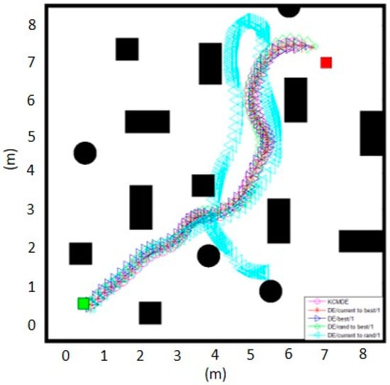
Figure 11.
Mobile robot trajectories using various algorithms in a complex environment.
5.3. Navigation Ability in Highly Complex and Special Environments
Highly complex and special environments were designed for testing the KNFC base on the KCMDE algorithm. Figure 12 illustrate the analysis of the sensor values and the two-wheel velocity in the highly complex environment. For example, the point A in Figure 13 corresponds to the point A in Figure 12. S1 is near the robot; however, the target is on the left of the robot. Therefore, the robot turns left (see LV and RV in Figure 13). At point B, S3 with a low value represents the obstacle on the right of the mobile robot. The velocity of the two wheels gradually decreases, and the velocity of the right wheel is marginally larger than that of the left wheel. The robot moves forward slowly. At point C, the mobile robot moves without obstacles, the velocity of the two wheels is large, and the robot turns toward the target gradually. At point D, the obstacle is on the left and the mobile robot thus turns right.
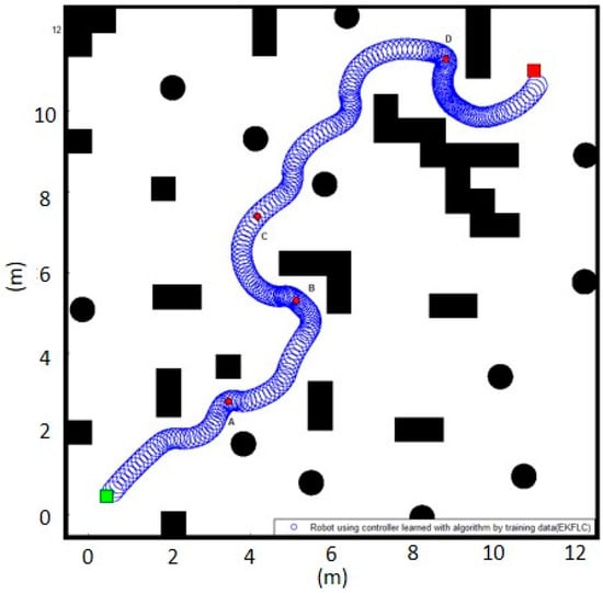
Figure 12.
Mobile robot trajectories using the KNFC base on the KCMDE algorithm in highly complex environments.
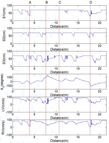
Figure 13.
Ultrasonic sensor values and velocities of the left and right wheels of the robot using the KNFC base on the KCMDE algorithm in highly complex environments.
In the special case environment, the threshold of A is set as 150° and the threshold of B is set as 90°. Figure 14 and Figure 15 illustrate the analysis in the special case environment. At point A, the angle between the direction of the mobile robot and the target is larger than threshold A. Thus, the mobile robot enters the wall-following mode. The line between point A and point B in Figure 14 indicates the angle between the direction of the mobile robot and the target is more than threshold B. Therefore, the mobile robot follows the wall. When the angle between the direction of the mobile robot and the target is equal to threshold B, the mobile robot navigates using the KNFC base on the KCMDE algorithm. At point C, the sensor groups S2 and S3 indicate that the obstacles are on the front and right of the robot. Because the obstacle to the right is near the robot, the robot turns left with low speed. (see LV and RV in Figure 14) At point D, the situation of the V-shaped environment is satisfied. In this situation, the sensor values become low and the target is on the left of the mobile robot. The velocity of the left wheel is nearly 0. The velocity of the right wheel is marginally higher than that of the left wheel but still low. The mobile robot slowly turns right in the V-shaped environment.
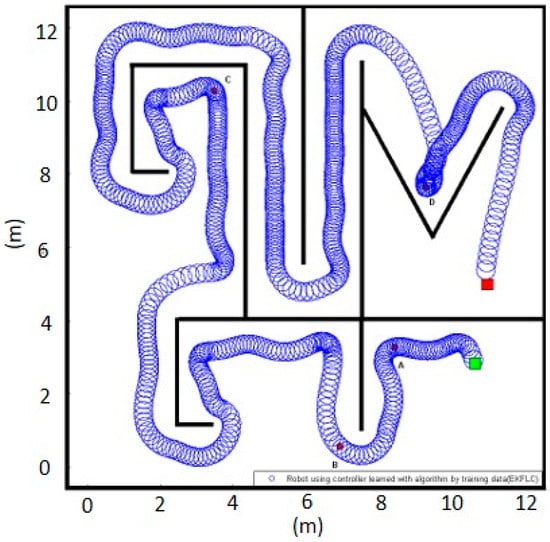
Figure 14.
Mobile robot trajectory using the KNFC base on the KCMDE algorithm in special environments.
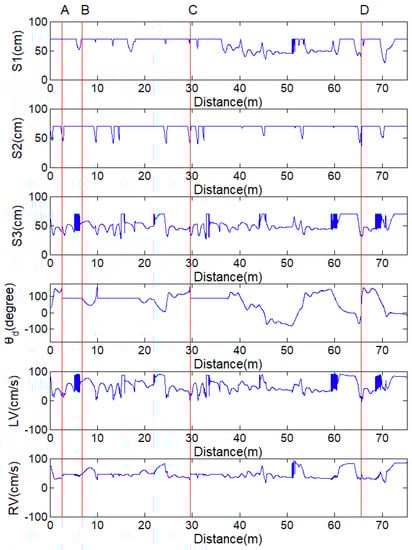
Figure 15.
Ultrasonic sensor values and velocities of the left and right wheels of the robot using the KNFC base on the KCMDE algorithm in special environments.
5.4. Implementation of Pioneer 3-DX Robots
Pioneer 3-DX robots were used to test the navigation ability of the proposed controller in complex, V-shaped, and U-shaped environments. Eight points were selected to describe the motion of the robot in each environment. In the complex environment (Figure 16), M1 was the panorama. Initially, the robot was at the start point (P1). The robot navigated through points P2, P3, P4, P5, and P6 and finally reached the target. Next, the robot was tested in the V-shaped environment (Figure 17), where M2 was the panorama. At P1, P2, and P3, the robot moved toward the target and encountered the V-shaped sac. Because the target was on the left of the robot, the robot turned right to avoid the obstacle. At P3 and P4, the angle between the robot and the target was larger than threshold A. Therefore, the robot entered the wall-following mode with a fixed target angle after threshold B. At P6, the angle between the robot and the target was equal to threshold B and the robot navigated using KNFC base on KCMDE algorithm. Finally, the robot reached the target (P7 and P8). The motion of the robot in the U-shaped environment in Figure 18 was similar to that in the V-shaped environment.
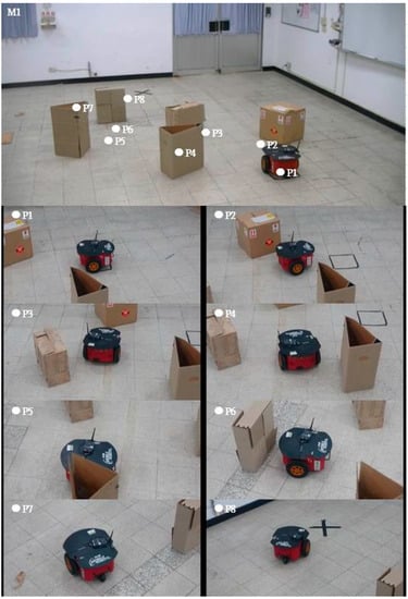
Figure 16.
Navigation of the Pioneer-3DX mobile robot in the case of a normal obstacle.
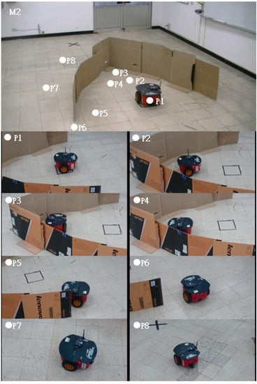
Figure 17.
Navigation of the Pioneer-3DX mobile robot in the case of a V-shaped obstacle.
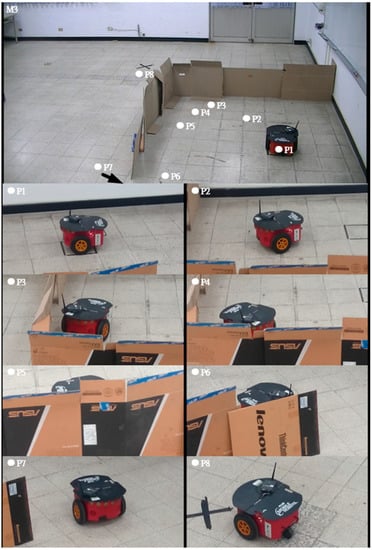
Figure 18.
Navigation of the Pioneer-3DX mobile robot in the case of a U-shaped obstacle.
6. Conclusions and Future Work
This study proposes a KNFC for mobile robot navigation control. In the proposed KNFC, a KCMDE is proposed to adjust the parameters of KNFC. The KCMDE algorithm combines the CA and DE strategy and is implemented using the knowledge sources of the belief space of the CA. For knowledge source selection, the concept of multi-strategy is used. The proposed KNFC is applied in PIONEER 3-DX mobile robots to achieve automatic navigation and obstacle avoidance capabilities. A novel escape approach is proposed to enable robots to autonomously avoid special environments. The angle between the obstacle and robot is used and two thresholds are set to determine whether the robot entries into the special landmarks and to modify the robot behavior for avoiding dead ends. The experimental results show that the proposed KNFC based on the KCMDE algorithm has improved the performance of learning ability, and system performance by 15.59%, and 79.01%, respectively, compared with the various DE methods. This study proved that the proposed method has a large SP value in high complex environments and an escape ability in special environments. Although the KNFC based on the KCMDE algorithm can perform mobile robot navigation control, several parameters of DE algorithms (such as DE/best/1, DE/current-to-best/1, DE/rand-to-best/1, and DE/current-to-rand/1) still need to be set in advance. Therefore, an adaptive adjustment method of these parameters will be developed in future work.
Author Contributions
Conceptualization, C.-H.C. and C.-J.L.; methodology, C.-H.C., C.-J.L. and S.-Y.J.; software, C.-H.C., C.-J.L. and S.-Y.J.; data curation, H.-Y.L. and C.-Y.Y.; writing—original draft preparation, C.-H.C., C.-J.L. and S.-Y.J.; funding acquisition, C.-J.L. All authors have read and agreed to the published version of the manuscript.
Funding
This research was funded by the Ministry of Science and Technology of the Republic of China, grant number MOST 109-2221-E-167-027.
Acknowledgments
The authors would like to thank the Ministry of Science and Technology of the Republic of China, Taiwan for financially sup-porting this research under Contract No. MOST 109-2221-E-167-027.
Conflicts of Interest
The authors declare no conflict of interest.
References
- Chen, C.-H.; Chen, W.-H. Bare-bones imperialist competitive algorithm for a compensatory neural fuzzy controller. Neurocomputing 2016, 173, 1519–1528. [Google Scholar] [CrossRef]
- Juang, C.-F.; Hsu, C.-H. Reinforcement Ant Optimized Fuzzy Controller for Mobile-Robot Wall-Following Control. IEEE Trans. Ind. Electron. 2009, 56, 3931–3940. [Google Scholar] [CrossRef]
- Juang, C.-F.; Chang, Y.-C. Evolutionary-Group-Based Particle-Swarm-Optimized Fuzzy Controller with Application to Mobile-Robot Navigation in Unknown Environments. IEEE Trans. Fuzzy Syst. 2011, 19, 379–392. [Google Scholar] [CrossRef]
- Kannaiyan, M.; Karthikeyan, G.; Raghuvaran, J.G.T. Prediction of specific wear rate for LM25/ZrO2 composites using Levenberg–Marquardt backpropagation algorithm. J. Mater. Res. Technol. 2020, 9, 530–538. [Google Scholar] [CrossRef]
- Juang, C.-F.; Lin, C.-T. An online self-constructing neural fuzzy inference network and its applications. IEEE Trans. Fuzzy Syst. 1998, 6, 12–32. [Google Scholar] [CrossRef]
- Dao, S.D.; Abhary, K.; Marian, R. An innovative framework for designing genetic algorithm structures. Expert Syst. Appl. 2017, 90, 196–208. [Google Scholar] [CrossRef]
- Ding, Y.; Zhang, W.; Yu, L.; Lu, K. The accuracy and efficiency of GA and PSO optimization schemes on estimating reaction kinetic parameters of biomass pyrolysis. Energy 2019, 176, 582–588. [Google Scholar] [CrossRef]
- Weskida, M.; Michalski, R. Finding influentials in social networks using evolutionary algorithm. J. Comput. Sci. 2019, 31, 77–85. [Google Scholar] [CrossRef]
- Alcaraz, J.; Landete, M.; Monge, J.F.; Sainz-Pardo, J.L. Multi-objective evolutionary algorithms for a reliability location problem. Eur. J. Oper. Res. 2020, 283, 83–93. [Google Scholar] [CrossRef]
- Xue, Y.; Li, M.; Shepperd, M.; Lauria, S.; Liu, X. A novel aggregation-based dominance for Pareto-based evolutionary algorithms to configure software product lines. Neurocomputing 2019, 364, 32–48. [Google Scholar] [CrossRef]
- Tuson, A.; Ross, P. Adapting Operator Settings in Genetic Algorithms. Evol. Comput. 1998, 6, 161–184. [Google Scholar] [CrossRef] [PubMed]
- Gomez, J.; Dasgupta, D.; González, F. Using Adaptive Operators in Genetic Search. Comput. Vis. 2003, 2724, 1580–1581. [Google Scholar] [CrossRef]
- Bryant, A.J. What Have You Done for Me Lately? Adapting Operator Probabilities in a Steady-State Genetic Algorithm. In Proceedings of the 6th International Conference on Genetic Algorithms, San Francisco, CA, USA, 15–19 July 1995; pp. 81–87. [Google Scholar]
- Peter, J.A. Adaptive and Self-adaptive Evolutionary Computations (1995). Available online: http://citeseerx.ist.psu.edu/viewdoc/summary?doi=10.1.1.6.4594 (accessed on 1 January 2020).
- Storn, R.; Price, K. Differential Evolution – A Simple and Efficient Heuristic for global Optimization over Continuous Spaces. J. Glob. Optim. 1997, 11, 341–359. [Google Scholar] [CrossRef]
- Kenneth, P.; Rainer, M.S.; Jouni, A.L. Differential Evolution: A Practical Approach to Global Optimization; Springer: Berlin, Germany, 2005. [Google Scholar]
- Yang, Y.; Chen, Y.; Wang, Y.; Li, C.; Li, L. Modelling a combined method based on ANFIS and neural network improved by DE algorithm: A case study for short-term electricity demand forecasting. Appl. Soft Comput. 2016, 49, 663–675. [Google Scholar] [CrossRef]
- Cheng, S.-L.; Hwang, C. Optimal approximation of linear systems by a differential evolution algorithm. IEEE Trans. Syst. Man Cybern. Part A Syst. Humans 2001, 31, 698–707. [Google Scholar] [CrossRef]
- Qin, A.K.; Huang, V.L.; Suganthan, P.N. Differential Evolution Algorithm with Strategy Adaptation for Global Numerical Optimization. IEEE Trans. Evol. Comput. 2008, 13, 398–417. [Google Scholar] [CrossRef]
- Robert, G.R. An introduction to cultural algorithms. In Proceedings of the Third Annual Conference on Evolutionary Programming, San Diego, CA, USA, 24–26 February 1994; pp. 131–139. [Google Scholar]
- Robert, G.R. Cultural Algorithms: Theory and Applications. New Ideas in Optimization; McGraw-Hill: Berkshire, UK, 1999. [Google Scholar]
- Coello, C.; Becerra, R. Evolutionary multiobjective optimization using a cultural algorithm. In Proceedings of the 2003 IEEE Swarm Intelligence Symposium. SIS’03 (Cat. No.03EX706), Indianapolis, IN, USA, 26 April 2003; pp. 6–13. [Google Scholar]
- Chen, C.-H. Compensatory neural fuzzy networks with rule-based cooperative differential evolution for nonlinear system control. Nonlinear Dyn. 2013, 75, 355–366. [Google Scholar] [CrossRef]
- Chen, C.-H.; Jeng, S.-Y.; Lin, C.-J. Mobile Robot Wall-Following Control Using Fuzzy Logic Controller with Improved Differential Search and Reinforcement Learning. Mathematics 2020, 8, 1254. [Google Scholar] [CrossRef]
- Lin, C.-J.; Jeng, S.-Y.; Lin, H.-Y.; Yu, C.-Y. Design and Verification of an Interval Type-2 Fuzzy Neural Network Based on Improved Particle Swarm Optimization. Appl. Sci. 2020, 10, 3041. [Google Scholar] [CrossRef]
- Lin, T.-C.; Chen, C.-C.; Lin, C.-J. Navigation control of mobile robot using interval type-2 neural fuzzy controller optimized by dynamic group differential evolution. Adv. Mech. Eng. 2018, 10, 1–20. [Google Scholar] [CrossRef]
- GitHub Source Code 2021. Available online: https://github.com/g951753321/KNFC_KCMDE (accessed on 3 February 2021).
Publisher’s Note: MDPI stays neutral with regard to jurisdictional claims in published maps and institutional affiliations. |
© 2021 by the authors. Licensee MDPI, Basel, Switzerland. This article is an open access article distributed under the terms and conditions of the Creative Commons Attribution (CC BY) license (http://creativecommons.org/licenses/by/4.0/).