Abstract
With the development of electronic infrastructures and communication technologies and protocols, electric grids have evolved towards the concept of Smart Grids, which enable the communication of the different agents involved in their operation, thus notably increasing their efficiency. In this context, microgrids and nanogrids have emerged as invaluable frameworks for optimal integration of renewable sources, electric mobility, energy storage facilities and demand response programs. This paper discusses a DC isolated nanogrid layout for the integration of renewable generators, battery energy storage, demand response activities and electric vehicle charging infrastructures. Moreover, a stochastic optimal scheduling tool is developed for the studied nanogrid, suitable for operators integrated into local service entities along with the energy retailer. A stochastic model is developed for fast charging stations in particular. A case study serves to validate the developed tool and analyze the economical and operational implications of demand response programs and charging infrastructures. Results evidence the importance of demand response initiatives in the economic profit of the retailer.
Keywords:
DC nanogrid; microgrid; electric vehicle; demand response; optimal scheduling; uncertainty 1. Introduction
The Smart Grid paradigm requires active participation and coordination of all the agents involved in the electric system [1,2]. With the advent of this concept, nanogrids (NGs) have emerged as an invaluable framework for the integration of renewable generation, electric vehicles (EVs), storage facilities and demand response (DR) programs [3,4,5,6]; as well as for electrical supplying of remote isolated areas [7]. In this context, the optimal coordination of the agents involved requires deploying advanced communication infrastructures and electronic interfaces on either AC, DC or hybrid networks [8,9,10]. Communication channels enable effective information exchange among the different assets that participate in the operation of the system. This novel paradigm allows to effectively coordinate the participation of the different agents, with the aim of pursuing more efficient management of the generation and storage facilities [11]; while consumers can also actively participate through DR initiatives, modifying their consumption profiles on the basis of price or incentive signals [12].
Because of the heterogeneity and conflicting interests of the different agents involved in the NG operation, their coordination is frequently addressed in a centralized fashion by the grid operator. This agent is usually integrated into the local service entity along with the local retailer [13]. In remote isolated areas, the local service entity usually owns the on-site generation and storage assets [14]. In such a case, the operator must ensure the supplying quality and reliability at minimum cost, in order to maximize the benefits obtained by the retailer. To this end, the operator can exploit public infrastructures such as charging stations [15,16], in order to complement the incomes obtained from energy supplying. Thereby, it is essential to operate the grid in an optimal way efficiently exploiting the different available resources and taking advantage of the flexibility provided by DR programs.
The optimal operation of NGs (or microgrids) is a hot topic that has attracted huge attention recently. In Ref. [17], the authors developed an optimal scheduling model for EVs and battery swapping stations. The model is formulated so that the costs of EVs are minimized while the profit of battery storage systems (BSSs) in energy markets is maximized. In Ref. [18], an energy management problem is formulated which considers renewable sources and an EV smart parking lot, with the objective of maximizing the EVs owner satisfaction. The authors in [19] developed a model predictive control for MGs which considers possible future variations in EVs demand. The possibility of vehicle-to-grid capabilities from EVs is considered in [20], by which bidirectional flows are enabled from/to the onboard storage systems. In Ref. [21], an operating window constrained strategic energy management is proposed for MGs, which allows different formulations depending is the problem is treated by the EVs owner or the MG operator. The reference [22] deals with the optimal operation of isolated MGs in which EVs are exploited as storage facilities, enabling vehicle-to-grid capabilities. The authors of [23] developed a bi-level optimization problem for isolated MGs equipped with battery swapping stations. The idea is to minimize the operating cost in the upper level while the secondary problem aims at maximizing the profits of the stations. In Ref. [24], an optimal scheduling model for industrial MGs with plug-in EVs is developed, in which constraints related to industrial production are included. Ref. [25] proposed a coordination model for charging stations supplied from photovoltaic (PV) panels, EV on-board storage and the rest of the isolated MG. In Ref. [26] the optimal generation scheduling is combined with the optimal reconfiguration of the grid. The reference [27] proposed a real time control scheme for a smart EV fleet for optimal coordination of vehicle-to-grid and grid-to-vehicle modes. In [28], the EV fleet is considered as a mobile storage system in a hierarchical real time model predictive control for MGs. The authors in [29] considered the control of a hybrid AC-DC MG in which the EV charging system is directly connected to the DC side. The authors of [30] developed a stochastic scheduling model for MGs, including EVs, renewable sources and fuel cells. The reference [31] proposed a multi-objective problem for optimal network reconfiguration, generation dispatch and capacitor switching in the presence of controllable loads and EVs. The reference [32] developed a two-level robust optimization framework for optimal scheduling of grid-connected MGs including plug-in EVs. Ref. [33] deals with the short-term optimal planning of MG layout considering plug-in EVs with enabled vehicle-to-grid capability. The authors of [34] exploited metaheuristic techniques to solve the optimal scheduling of an MG with renewable sources, EVs and battery energy storage systems (BES). The authors of [35] considered three different charging modes for plug-in EVs, analyzing their impact on the MG optimal scheduling task. Ref. [36] analyzed the role of EVs for critical load restoration in resilient MGs, exploiting vehicle-to-grid and grid-to-vehicle capabilities as well as onboard high-powered engine generators.
As deduced from the review above, optimal scheduling of MGs is essential to minimize their operating costs or maximizing their monetary profits. In this sense, flexible loads such as charging stations and DR initiatives play a vital role to boost up the efficiency of the system. To maximize the penetration of EVs, DC NGs emerge as the optimal solution for reducing system requirements. By this approach, charging stations can be directly connected to the DC bus through DC-DC converters, thus allowing a simplification in their control schemes. This paper develops an optimal day-ahead scheduling model for DC isolated NGs, which is suitable for grid operators that are integrated into the local service entity structure along with the local retailer. This way, in contrast to most of the existing scheduling tools for similar grids which are devoted to minimizing the operational cost, the developed formulation aims at maximizing the benefits obtained by the retailer optimally coordinating on-site generators, storage facilities, flexible consumers and public charging infrastructures. In addition, the proposed model incorporates various uncertainties, which are modeled as stochastic parameters, including the charging station demand for which, in contrast to other approaches which model the stochastic EV charging demand using conventional probability functions, a specific stochastic model is developed. For the sake of clarity, the major contributions of this paper are summarized below:
- Describing a DC layout for isolated NGs with DR programs and public EV charging stations.
- Developing an optimal day-ahead scheduling model for the grid system described, which is suitable for a grid operator which is integrated into the local service entity structure along with the local retailer.
- Developing a stochastic model for the different uncertainties involved in the NG operation, including renewable generation, local demand and EV charging profiles.
- Analyzing the influence of DR programs and EV penetration in the NG operation, also focusing on the economic impact of such aspects.
In the rest of the paper, Section 2 describes the analyzed NG layout, the agents involved and their role in NG operation. Section 3 presents the developed optimal scheduling model for the NG described in the previous section. Section 4 develops a stochastic framework for considering uncertainties in renewable generation, demand and EV charging profiles. Section 5 presents various case studies. The main conclusions are duly drawn in Section 6.
2. Description of the NG under Study
As commented, this paper is focused on isolated DC NGs. This kind of system involves the participation of various agents. The more notable interactions among the agents involved are depicted in Figure 1, while their roles are explained below:
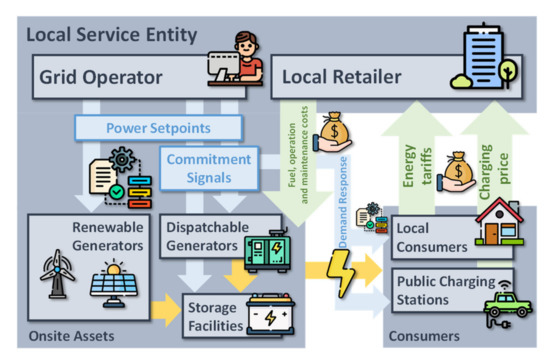
Figure 1.
Pictorial representation of the agents involved in the operation of the NG under study and the more notable interactions among them.
- NG operator: this agent is integrated into an upscale structure called a local service entity. It is responsible for operating the grid in an optimal way, ensuring the supplying quality and reliability. To this end, this agent daily performs a day-ahead optimal scheduling plan, by which the different on-site assets are coordinated with DR premises, such as those enabled by flexible consumers and public charging infrastructures. As a result, commitment signals, power set-points and DR information are sent to generators, storage systems and flexible consumers to address the resulted scheduling plan.
- Retailer: this agent provides fuel for conventional generators and is responsible for the monetary expenditures derived from generator operation (operation and maintenance). On the other hand, it receives monetary incomes from consumers through energy tariffs and public charging infrastructures, of which the local service entity is the owner.
- Generators and storage facilities: they are on-site assets owned by the local service entity. They may be formed by conventional generators, such as diesel engine generators (DEGs); renewable generators, such as PV panels or wind turbines (WTs); and storage facilities like BES.
- Consumers: residential demand and public charging infrastructures are considered as consumers in this paper. The residential demand comprises inelastic and flexible consumption. While the first one does not respond to price or incentive signals from the NG operator, the second one may be scheduled in order to increase the efficiency of the system or ensure its reliability. On the other hand, public charging stations are owned by the local service entity. They provide adequate charging infrastructures to privately owned EVs, obtaining a monetary counterpart which is received by the retailer.
To effectively address the optimal coordination of the different participants, both energy and communication channels have to be enabled, which are illustrated in Figure 2. Each controllable agent is connected through electronic interfaces, which allow an effective energy flow control from/to the different elements. This way, PV arrays, charging points and BES are directly connected to the DC bus through DC-DC converters. On the other hand, DEG and WTs require a rectified stage, which converts the generated AC waveform to DC. It is assumed that residential consumers mostly comprise DC loads; therefore, they can be connected directly to the DC bus without the necessity of an interface. In contrast, flexible consumers require a control mechanism that receives the commitment signals emitted from the NG operator. Each day, the operator receives forecasted data for weather and demand, which allow the performance of an optimal scheduling plan for the grid. This plan is transferred to the conventional generators and storage systems in the form of commitment and set-point signals, while renewable sources receive power set-points. DR programs are enabled through direct communication with flexible consumers. Thereby, the public charging station may be controlled through power set-points, so that EV demand may be totally satisfied or not, while flexible residential consumers can be actually scheduled, shifting their consumption to the more convenient hours of the day.

Figure 2.
Layout of the NG under study.
3. Optimal Scheduling Model for the NG under Study
In this section, the mathematical formulation for the optimal scheduling of the NG described in Section 2 is developed. The optimization problem is formulated as Mixed-Integer-Lineal programming, which can be solved using conventional solvers.
3.1. Assumptions
It has been widely reported that electronic devices can delay the response of the device to which it is interconnected by several seconds [37]. This aspect was not considered in the developed formulation because it was assumed that the time step scheduling is considerably larger than the delay introduced by electronic devices. This way, this aspect did not impact the scheduling result yielded by the developed tool.
3.2. Objective Function
The optimal scheduling problem is formulated from the retailer point of view, which aims at maximizing its own profit. To this end, this agent obtains monetary incomes from serving energy in flexible and non-flexible consumers as well as charging processes in EV stations. On the other hand, this agent incurs monetary expenditures due to fuel consumption of DEG and operation-derived costs of the other generation and storage assets. Keeping this in mind, the objective formulation can be formulated as follows:
where stands for the representative scenario set; is the probability of the scenario; is the time step; is the set of time intervals; is the energy cost (energy tariffs); is the expected demand; the superscript EV makes mention to electric vehicles; is the set of shiftable consumers; is a binary variable that indicates the commitment status; stands for power; is the operation and maintenance costs; and the superscripts PV, WT, BES and DEG make mention to solar panels, wind generators, battery storage and diesel engine, respectively.
The objective formulation is formulated considering a stochastic model for uncertainties so that the expression (1) considers the probability of occurrence of each scenario. The first term of the incomes stands for the energy consumption of inelastic residential consumers, the second term counts the profit from EV charging and the last element represents the payments of flexible consumers.
The monetary expenditures mainly comprise operation and maintenance costs of generation assets. For renewable-based generators, these costs are proportional to the energy generated [7], whereas, in the case of BES, they are quadratic functions of the energy exchanged with the grid [38]. The last element of the expenditures stands for the fuel cost of DEG, which can be calculated as a quadratic function of the energy generated, as follows [39]:
where , and are predefined coefficients.
In order to keep the lineal feature of the developed problem, quadratic functions can be efficiently linearized using piecewise representations [15] (see Appendix A).
3.3. DEG Modelling
DEG units can be modeled as other dispatchable generators by their upper and lower-rated values and ramping constraints, as said the Equations (3) and (4), respectively.
where and are the minimum and maximum dispatchable powers of the DEG and is the ramping rate.
3.4. PV Modelling
PV generation is influenced by uncertain parameters such as solar irradiation and ambient temperature. Assuming these parameters are known or sufficiently well-predicted, the available power generation can be calculated using an available PV array model. In this paper, the model considered in [7,14] is used, which determines the PV generation capacity as a function of the solar irradiation and ambient temperature, as follows:
where is the rating power of the PV array; is the solar irradiance; is the ambient temperature and is the efficiency of PV panels.
As pointed out in [7,14], model (5) does not take into account the installed power of the PV generators. In other words, the second term in (5) may be higher than 1, which yields a value higher than the rated power of PV panels. In practice, inverters impose limitations in the PV power generation to avoid failure or fast degradation of components. Traditionally, the equipment allows exceeding the nominal power by 10% [40], assuming that these overvalues may be eventually assumed without excessively deteriorating the components of the PV array. With these premises, the PV array model is completed with (6).
It is worth noting that the developed model considers the PV generation as a variable of the problem. It means that the NG operator can schedule its production on the basis of forecasted data. In this sense, the scheduling result may occasionally set the PV generation below the available power calculated by (5). In such a case, the surplus energy is assumed to be dissipated in dummy loads [41,42].
3.5. WT Modelling
As in the case of the PV panels, the power given by a WT depends on the available wind speed. Once this parameter is known or approximated, the available wind generation can be estimated on the basis of the wind speed-power curve of WTs [7]. A typical graph for this kind of curve is shown in Figure 3. It can be distinguished into three clear zones. For a wind speed below , the turbine is not able to extract energy from the wind and therefore, the power produced is zero. After surpassing this threshold, the power given by the turbine increases until reaching the rated power of the device at , which is a characteristic value of each turbine model. Beyond this point, the turbine is able to give its rated power until a maximum threshold , beyond which the turbine is braked to avoid breakdowns. The wind speed-power curve of a WT is typically represented by a set of equations as shown in (7), while the expression (8) takes into account the efficiency of the coupling rectifier.
where is the wind speed; and are the minimum and maximum wind speed values for which the WT can work; is the nominal wind speed of WT; and are predefined coefficients; is the rated power of WT; and is the efficiency of WT.

Figure 3.
Typical wind speed-power curve of a WT.
3.6. BES Modelling
The power that a BES can exchange with the system is typically upper bounded, as said the constraint (9), whose nominal values are determined by the nominal capacity and the energy to power ratio [43]. It is realistic to assume that charging and discharging processes are actually complementary, which is ensured by imposing the constraint (10). Equation (11) models the state of charge of the batteries, which is limited by their nominal capacity and depth of discharge settings [40], as said the Equation (12).
where is the energy stored in batteries; is the efficiency of batteries; is the nominal capacity of the storage system; is the depth of discharge; and the superscripts and stand for the charging and discharging processes of batteries, respectively.
Equation (11) models the energy stored in batteries as a function of the state of charge at and the total energy exchanged with the grid. However, as pointed out in other studies [7,40], this model has to be completed by setting the state of charge at the beginning of the time horizon. As customary (e.g., see [41]), it is assumed in this work that the BES is fully charged at the beginning of the time horizon. In addition, to keep the model coherent, the state of charge of the BES is forced to be equal to the nominal capacity at the end of the time horizon. These working conditions are ensured by imposing the constraint (13).
3.7. Shiftable Consumers Modeling
As commented previously, it is considered that a part of the local demand may respond to commitment signals emitted by the NG operator. This kind of responsible load can therefore adjust their scheduling programs to achieve a more efficient operation of the grid. As in other related problems [14], it is assumed that these consumers have to be operated continuously, which means, once their operating cycle has started, it cannot be interrupted until completing their duty cycle, as modeled the Equation (14).
where and are binary variables that indicate the activation/deactivation of a shiftable consumer.
It is assumed that these consumers have some preferences about when they prefer to be scheduled, in this sense, they have to be operated within allowable time windows, the scheduling tool being free to schedule their consumption in those time ranges. The constraint (15) ensures that shiftable consumers complete their duty cycles within the considered time windows. The model has to be completed by Equations (16) and (17), which ensure that responsible loads cannot be scheduled out of their time windows and are activated once over the time horizon, respectively.
where is the total number of time slots that a shiftable consumer must be connected throughout a day.
On the other hand, and with the aim of completing the analysis, it has been also considered the case in which the shiftable loads could not be operated in a flexible manner. In such a case, it is assumed that these consumers desire to start their operation at the first slot of the allowable time window, which is ensured by the model (18)–(20).
3.8. Public EV Charging Station Modeling
The developed model assumes the public charging station can be operated in a flexible manner, however, in contrast to the flexible consumers considered in the previous section, the charging points response in this case to set-point signals rather than commitment orders, as said in Equation (21).
By the model (21), the expected EV demand may be only partially satisfied. This way, the operator has the capability to decide if it is necessary to not fully cover or even ignore some charging events, whether this supposes an actual benefit for the grid operation.
3.9. NG Balance
The energetic balance is ensured each time step by the constraint (22), which establishes the generation-consumption equilibrium. In this case, the non-served load was not contemplated, thus having to satisfy the inelastic expected demand entirely. Therefore, DR is in this case enabled by shiftable consumers and the public charging infrastructure.
3.10. Optimization Problem
The optimal scheduling model developed above is formulated from the retailer point of view, which aims at maximizing their profits while the operator ensures the quality of supplying. In this sense, the model is formulated as a maximization problem in which (1) supposes the objective function. Therefore, the result of the problem searches for the optimal scheduling of the different controllable assets that maximizes the monetary incomes of the retailer. For the sake of analyzing, a case was also considered in which the shiftable consumers cannot be operated in a flexible way, minimizing the DR capability of the system. Both problems are stated below.
Model 1: shiftable consumers can be operated in a flexible fashion
Subject to: (3)–(14) and (18)–(22).
Model 2: flexible operation of shiftable consumers is not enabled
Subject to: (3)–(17), (21) and (22), where stands for the vector of decision variables (see Nomenclature).
4. Uncertainties Modeling
The optimal scheduling model developed in Section 3 contemplates various uncertain parameters, which are reported in Table 1. For managing such parameters, a stochastic framework has been proposed. Stochastic modeling is based on representing the uncertain parameters by means of probability distributions, from which one can generate a number of scenarios [44]. The scenarios generated constitute the scenario-space (), which has to be formed by many members since a large number of scenarios have to be considered to properly catch the stochastic essence of the parameter (normally 1000 [45]). Because of the large size of the scenario space, the optimization model may be intractable in practice. Indeed, one should note that all the variables and constraints would have size . To overcome such issues, some papers have proposed to use scenario reduction approaches [14,45]. By these techniques, the original space is completely described by just a set of few representative members, which are considered a sufficiently descriptive image of the original space. Among the available space reduction approaches, clustering techniques are quite popular because of their efficiency, adaptability accuracy and simplicity [46]. Specifically, the k-medoids method has been used in this paper because of its overall good performance [46]. The k-medoids method is inspired by the optimal plant location problem. In such a problem, a set of plants must be placed in a set of cities, so that the total distance from the plants in the cities is minimized. This approach thus grouping the set of scenarios into clusters, so that each cluster is fully described by just a member within it called medoid. This way, the scenario space is reduced to the so-called representative scenario-space (), which is a notably smaller scale. The k-medoid method presents a degree of freedom, namely the total number of clusters to be created. To set this parameter, helpful indicators such as the total sum of distances and the Davies–Bouldin index along the methodology described in [47] have been used. The flowchart in Figure 4 summarizes the steps necessary for solving the optimal scheduling problem developed in Section 3 with stochastic modeling of uncertainties. One of the most interesting features of the k-medoids method is the possibility of easily calculating the probability of occurrence of each scenario, as follows:
where is the scenario space; and represents the cluster of the representative scenario.

Table 1.
Uncertain parameters involved in the operation of the NG under study.

Figure 4.
Proposed flowchart for solving the proposed optimal scheduling problem with stochastic modeling of uncertainties.
It remains to be explained how the different uncertain parameters involved are modeled on the basis of probability functions, which is explained in the following sections.
4.1. Predictable Parameters
Some uncertain parameters can be day-ahead forecasted with sufficient accuracy [39]. Examples of these profiles are weather parameters or inflexible demand. For these kind of uncertainties, the forecasted data can be subjected to errors derived from the forecast technique or unpredictable events. Such errors can be modeled as normal distributions [48], taking the forecasting parameter as mean and a pre-set standard deviation. Using this distribution function, the scenario space can be generated for these parameters. For the model developed here in particular, the inflexible demand, solar irradiation, temperature and wind speed are assumed to be managed by this approach [38,49,50].
4.2. EV Demand Modeling
In contrast to the other uncertain parameters, the EV demand, especially at low-aggregated levels, is hardly predictable due to the generally random behaviors of drivers. In this sense, some references have considered specific probability distributions for EV demand [16,51,52]. For the particular case of the NG under study, it is important to note that at this scale the majority of consumers are domestic. In this sense, it was considered that the public charging station is devoted to light vehicles (cars and motorbikes).
In this paper, a stochastic model for the considered public charging stations has been developed. The developed model is based on the vehicle trip distribution (), which is shown in Figure 5 for a typical weekday in US [16]. This distribution indicates the probability of an EV is driving on road at each hour of the day. It is realistic to assume that the probability of charging events will increase with the probability of a vehicle driving on the road [16]. Thus, the probability of charging events each hour of the day can be adjusted to the probability distribution shown in Figure 5.
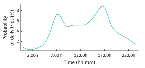
Figure 5.
U.S. vehicle trip distribution on weekdays [16].
On the other hand, it is necessary to model the number of charging events that may occur in a day. It is assumed that this parameter can be either predicted based on historical data or directly estimated from for example market studies. In this sense, the number of daily charging events () is modeled with a normal distribution, where the mean stands for the daily expected number of charging events and models the standard deviation, as follows:
where is a function that yields the nearest integer; is a function that yields a random number based on a probability function; and is a normal distribution with mean and standard deviation .
Once the total number of charging events was determined, it can be used as the entry of the vehicle trip distribution, in order to determine the arrival time of each vehicle, as follows:
Now, the vector can be used to construct the vector , whose element is equal to 1 if a vehicle arrives at the charging station at the time instant and 0 otherwise, using the following simple loop:
Now, the vector can be used for modeling the EV demand, as follows:
where is the rated power of the charging process.
The model (29) considers two plausible assumptions:
- The EV demand is considered constant during all the charging processes which, as indicated in [15], is a quite realistic assumption since only marginal variations with respect to the rating values are observed during the short time of the charging event.
- The EV charging process is completed within a unique time slot, which is quite realistic, assuming fast charging processes, which can be completed in only 15–30 min [15].
Nevertheless, it is worth mentioning that the developed stochastic model for EV demand presents a modular structure that allows it to be adapted to any charging mode or more comprehensive charging profiles. Nevertheless, it has been assumed that the developed model is quite realistic and useful in practice, lying out of the scope of this work further analyzing other more elaborated models. For the sake of example, Figure 6 plots some EV demand profiles constructed with the developed model considering various numbers of expected charging events. In this figure, fast charging mode was considered, with 55 kW rated power [15].

Figure 6.
EV demand scenarios generated with the developed stochastic model for various numbers of expected charging events.
5. Case Study
This section presents a case study that is devoted to validating the developed stochastic optimal scheduling formulation, for the DC NG layout described in Section 2. The optimization model was coded in Matlab R2019a and solved using Gurobi [53] with 30-min resolution.
5.1. Data
For creating the scenarios for uncertain parameters, several public databases were used. Figure 7 shows the forecasted profiles for the solar irradiance, temperature, local demand and wind speed along the scenarios generated using the methodology described in Section 4. The considered weather profiles were taken from Ref. [54] and correspond with real data observed at the Virgin Islands on 3 May 2016. The forecasted profile corresponding to local demand was adapted from real demand measurements at La Palma Island at the same date, which is available in [55].
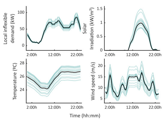
Figure 7.
Forecasted profiles (solid lines) and scenarios (discontinuous lines) used for modelling uncertain parameters in simulations.
The data corresponding to the other parameters involved are reported in Table 2, while the data regarding shiftable consumers are collected in Table 3. For the EV charging the fast mode was considered, with a rated power of 55 kW and a price of 1.5 $/kWh [15]. Finally, Figure 8 shows the Time-of-Use tariff used for non-flexible consumers, which is based on typical dynamic tariffs [14].
Table 2.
Parameters considered in simulations [7,14,38,39].
Table 3.
Data of shiftable consumers.

Figure 8.
Time-of-Use tariff applied to non-shiftable consumers in simulations.
5.2. Results
In this section, various results are presented and commented on. For further analysis, the operation of the NG under study is considered with and without flexibility in shiftable loads (models 1 and 2, respectively). Moreover, the model is tested for various numbers of expected charging events ( in Equation (26)). Figure 9 shows the value of the objective function (retailer profit) for various cases. As observed, the flexibility provided by consumers has a direct impact on economical profitability. In fact, the monetary balance for the retailer resulted in negative values (monetary losses) if the shiftable consumers are operated in a rigid manner, while the benefits may achieve up to ~400$ in the case of the flexible program. Logically, the profitability of the system grows with the number of expected charging events, since more monetary incomes are obtained from the public charging station, as seen in Figure 10.

Figure 9.
The value of the objective function for various scenarios.

Figure 10.
Monetary incomes obtained from EV charging processes in various scenarios.
As seen in Figure 9, the flexibility of shiftable consumers has a direct impact on the profitability of the system. This is due to the flexibility provided by consumers allows to further satisfy the expected EV demand. Indeed, as observed in Figure 11, the EV demand satisfaction decreases in the case of considering the model, in which demand flexibility is not enabled. In order to further analyze the behavior of the charging station, Figure 12 plots the expected and actual satisfied EV demand with model 2, as seen in this figure. Some expected charging events were not covered, while others were just partially satisfied.
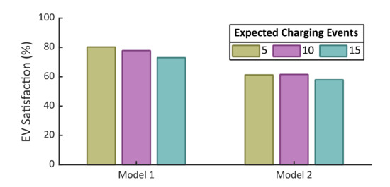
Figure 11.
Percentage of the expected EV demand actually satisfied in various scenarios.
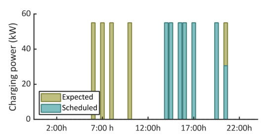
Figure 12.
Expected and actual satisfied EV demand without considering flexibility (model 2).
In order to further analyze the role of the shiftable consumers, their scheduling results are plotted in Figure 13 considering the optimization models 1 and 2. As seen, in the case of flexible operation, both consumers are scheduled later, exploiting higher PV penetration and avoiding the use of DEG.
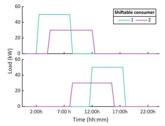
Figure 13.
Scheduling result of the shiftable consumer with model 1 (upper) and 2 (bottom).
As commented, the main advantage of operating the shiftable consumers in a flexible way is reducing the dependency on costly generators like DEG. As seen in Figure 14, the expected DEG generation with flexibility barely surpassed 400 kWh, while it was higher than 600 kWh in case of no flexibility. These results are traduced in lower fuel consumption and therefore lower operational cost. As seen in Figure 15, the expected fuel cost with model 1 did not surpass 400$, while the fuel cost was higher than 800$ in the case of the rigid operation of shiftable consumers. These results have also a direct impact on environmental concerns since, as commented in [40], total CO2 emissions are proportional to diesel consumption.

Figure 14.
Total DEG generation in various scenarios.
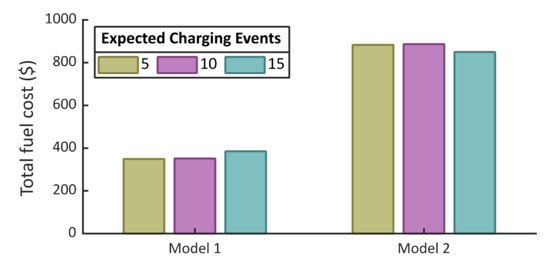
Figure 15.
Total fuel cost in various scenarios.
6. Conclusions and Future Works
This paper has comprehensively analyzed a possible DC isolated nanogrid layout for integration of renewable sources, energy storage facilities, demand response initiatives and electric vehicle charging infrastructures. In this sense, the necessary electronic interfaces and communication channels have been described. Moreover, the relationship among the different agents involved in the grid operation has been discussed. An optimal scheduling tool for the analyzed nanogrid has been presented, along with a stochastic framework for uncertainties modeling. In this regard, a specific stochastic model for fast charging stations has been developed.
A case study has been presented and various results have been commented, with the aim of validating the developed formulation and analyzing the impact of demand response programs in the grid operation. The results obtained have served to evidence the importance of flexible consumption for boosting up the monetary incomes of the retailer and reducing diesel consumption and therefore CO2 emissions. It has been also remarkable the role of public charging infrastructures in the profitability of the grid and how demand response programs affect their viability.
Future works should be focused on analyzing the considered grid layout in grid-connected mode, for which the uncertainty of energy pricing along with the possibility of selling energy to the upscale grid has to be considered.
Author Contributions
Conceptualization, S.A.H., M.T.-V. and R.A.T.; methodology, S.A.H., M.T.-V., H.M.H. and W.K.M.; software, M.T.-V., H.M.H. and R.A.T.; validation, M.T.-V., H.M.H. and F.J.; formal analysis, M.T.-V., H.M.H. and R.A.T.; investigation, S.A.H. and M.T.-V.; resources, H.M.H., R.A.T. and F.J.; data curation, S.A.H., M.T.-V. and W.K.M.; writing—original draft preparation, S.A.H., M.T.-V. and W.K.M.; writing—review and editing, H.M.H., R.A.T. and F.J.; visualization, M.T.-V., H.M.H. and W.K.M.; supervision, H.M.H., W.K.M. and F.J.; project administration, W.K.M. and F.J.; funding acquisition, H.M.H., R.A.T. and F.J. All authors have read and agreed to the published version of the manuscript.
Funding
This research received no external funding.
Acknowledgments
The icons used in the figures of this paper were developed by Freepik, ultimatearm, monkik and smalllikeart from www.flaticon.com (accessed on 16 September 2021).
Conflicts of Interest
The authors declare no conflict of interest.
Nomenclature
| Indexes (Sets) | |
| Time | |
| Scenario | |
| Representative scenario | |
| Shiftable load | |
| Cluster of the representative scenario | |
| Time window of a shiftable load | |
| Superscripts | |
| Diesel engine generator | |
| Electric vehicle | |
| Photovoltaic | |
| Wind turbine | |
| Battery energy storage in charging/discharging mode | |
| Maximum minimum value of a variable or parameter | |
| Constants and parameters | |
| Time step (h) | |
| Energy price ($/kWh) | |
| Predicted local demand (kW) | |
| Operation and maintenance cost ($/kWh or $/kWh²) | |
| Fuel cost coefficients ($/h, $/kWh, $/kWh²) | |
| Ramping rate (kW) | |
| Solar irradiance (kW/m²) | |
| Ambient temperature (ºC) | |
| Efficiency (pu) | |
| Wind speed (m/s) | |
| Speed-power wind turbine curve coefficients (kW·(m/s)−3, -) | |
| Total number of hours of operation of shiftable load (h) | |
| EV demand modeling | |
| Normal distribution (with mean and standard deviation ) for modeling the daily number of charging events | |
| Total number of charging events | |
| Arrival time of the vehicle corresponded to the scenario | |
| Binary vector whose element is equal to 1 if a vehicle arrives at the charging station at the time instant and 0 otherwise | |
| Function that returns a random number based on a probability distribution function | |
| Function that rounds to the nearest integer | |
| Vehicle trip distribution | |
| Rated power of Electric vehicles charging (kW) | |
| Decision variables | |
| Power (kW) | |
| Commitment status (binary) | |
| Energy stored (kWh) | |
| Flag variable that indicates the activation/deactivation of a shiftable load (binary) | |
Appendix A. Linearization of Quadratic Terms
In the developed optimization model, some quadratic terms have appeared in the objective function. To linearize these terms and, therefore preserve the lineal character of the problem, a piecewise representation of such variables has been considered. By this approach, the quadratic function is characterized by its piecewise representation , for which () points are taken, as follows:
Usually, the higher number of points considered, the more accurate the piecewise representation is however, the optimization problem becomes computationally more expensive. The piecewise representation of quadratic terms allows to replace them by the dummy variable wherever they appear in the problem. This variable is calculated, as follows:
where is a binary variable that ensures that only one segment of the piecewise curve is activated at once by imposing the following constraint:
To ensure that only one segment of the piecewise curve is activated at once, the following constraint must be imposed:
In (A2), the parameters and can be calculated as follows:
Finally, it is important to note that (A2) involves the product of two variables ( and ), which introduces further nonlinearities in the model. To avoid this issue, the product of variables can be replaced by the lineal variable for which the following additional constraints are needed:
where is a large positive constant.
References
- Mohammadi, F. Emerging Challenges in Smart Grid Cybersecurity Enhancement: A Review. Energies 2021, 14, 1380. [Google Scholar] [CrossRef]
- Khalid, H.; Shobole, A. Existing Developments in Adaptive Smart Grid Protection: A Review. Electr. Power Syst. Res. 2021, 191, 106901. [Google Scholar] [CrossRef]
- Shen, Y.; Fang, W.; Ye, F.; Kadoch, M. EV Charging Behavior Analysis Using Hybrid Intelligence for 5G Smart Grid. Electronics 2020, 9, 80. [Google Scholar] [CrossRef] [Green Version]
- Aluisio, B.; Dicorato, M.; Ferrini, I.; Forte, G.; Sbrizzai, R.; Trovato, M. Planning and reliability of DC microgrid configurations for Electric Vehicle Supply Infrastructure. Int. J. Electr. Power Energy Syst. 2021, 131, 107104. [Google Scholar] [CrossRef]
- Khan, M.U.; Wali, K.; Karimov, K.S.; Saeed, M.A. A new proposed hierarchy for renewable energy generation to distribution grid integration. In Proceedings of the 2015 International Conference on Emerging Technologies (ICET), Peshawar, Pakistan, 19–20 December 2015; pp. 1–6. [Google Scholar] [CrossRef]
- Saeed, M.A.; Ahmed, N.; Hussain, M.; Jafar, A. A comparative study of controllers for optimal speed control of hybrid electric vehicle. In Proceedings of the 2016 International Conference on Intelligent Systems Engineering (ICISE), Islamabad, Pakistan, 15–17 January 2016; pp. 1–4. [Google Scholar] [CrossRef]
- Arévalo, P.; Tostado-Véliz, M.; Jurado, F. A novel methodology for comprehensive planning of battery storage systems. J. Energy Storage 2021, 37, 102456. [Google Scholar] [CrossRef]
- Smadi, A.A.; Ajao, B.T.; Johnson, B.K.; Lei, H.; Chakhchoukh, Y.; Abu Al-Haija, Q. A Comprehensive Survey on Cyber-Physical Smart Grid Testbed Architectures: Requirements and Challenges. Electronics 2021, 10, 1043. [Google Scholar] [CrossRef]
- Lázaro, J.; Astarloa, A.; Rodríguez, M.; Bidarte, U.; Jiménez, J. A Survey on Vulnerabilities and Countermeasures in the Communications of the Smart Grid. Electronics 2021, 10, 1881. [Google Scholar] [CrossRef]
- Romano, G.; Mantini, G.; Di Carlo, A.; D’Amico, A.; Falconi, C.; Wang, Z.L. Piezoelectric potential in vertically aligned nanowires for high output nanogenerators. Nanotechnology 2011, 22, 465401. [Google Scholar] [CrossRef]
- Nasir, T.; Bukhari, S.H.H.; Raza, S.; Munir, H.M.; Abrar, M.; ul Muqeet, H.A.; Bhatti, K.L.; Ro, J.-S.; Masroor, R. Recent Challenges and Methodologies in Smart Grid Demand Side Management: State-of-the-Art Literature Review. Math. Probl. Eng. 2021, 2021, 5821301. [Google Scholar] [CrossRef]
- Iqbal, S.; Sarfraz, M.; Ayyub, M.; Tariq, M.; Chakrabortty, R.K.; Ryan, M.J.; Alamri, B. A Comprehensive Review on Residential Demand Side Management Strategies in Smart Grid Environment. Sustainability 2021, 13, 7170. [Google Scholar] [CrossRef]
- Paterakis, N.G.; Erdinç, O.; Bakirtzis, A.G.; Catalão, J.P.S. Optimal Household Appliances Scheduling Under Day-Ahead Pricing and Load-Shaping Demand Response Strategies. IEEE Trans. Ind. Inform. 2015, 11, 1509–1519. [Google Scholar] [CrossRef]
- Tostado-Véliz, M.; Mouassa, S.; Jurado, F. A MILP framework for electricity tariff-choosing decision process in smart homes considering ‘Happy Hours’ tariffs. Int. J. Electr. Power Energy Syst. 2021, 131, 107139. [Google Scholar] [CrossRef]
- Tostado-Véliz, M.; Arévalo, P.; Jurado, F. A Comprehensive Electrical-Gas-Hydrogen Microgrid Model for Energy Management Applications. Energy Convers. Manag. 2021, 228, 113726. [Google Scholar] [CrossRef]
- Negarestani, S.; Fotuhi-Firuzabad, M.; Rastegar, M.; Rajabi-Ghahnavieh, A. Optimal Sizing of Storage System in a Fast Charging Station for Plug-in Hybrid Electric Vehicles. IEEE Trans. Transport. Electrif. 2016, 2, 443–453. [Google Scholar] [CrossRef]
- Zhang, M.; Chen, J. The Energy Management and Optimized Operation of Electric Vehicles Based on Microgrid. IEEE Trans. Power Deliv. 2014, 29, 1427–1435. [Google Scholar] [CrossRef]
- Honarmand, M.; Zakariazadeh, A.; Jadid, S. Integrated scheduling of renewable generation and electric vehicles parking lot in a smart microgrid. Energy Conver. Manag. 2014, 86, 745–755. [Google Scholar] [CrossRef]
- Ji, Z.; Huang, X.; Xu, C.; Sun, H. Accelerated Model Predictive Control for Electric Vehicle Integrated Microgrid Energy Management: A Hybrid Robust and Stochastic Approach. Energies 2016, 9, 973. [Google Scholar] [CrossRef]
- Mortaz, E.; Valenzuela, J. Microgrid energy scheduling using storage from electric vehicles. Electr. Power Syst. Res. 2017, 143, 554–562. [Google Scholar] [CrossRef]
- Panwar, L.K.; Konda, S.R.; Verma, A.; Panigrahi, B.K.; Kumar, R. Operation window constrained strategic energy management of microgrid with electric vehicle and distributed resources. IET Gener. Transm. Distrib. 2017, 11, 615–626. [Google Scholar] [CrossRef]
- Singh, S.; Jagota, S.; Singh, M. Energy management and voltage stabilization in an islanded microgrid through an electric vehicle charging station. Sustain. Cities Soc. 2018, 41, 679–694. [Google Scholar] [CrossRef]
- Li, Y.; Yang, Z.; Li, G.; Mu, Y.; Zhao, D.; Chen, C.; Shen, B. Optimal scheduling of isolated microgrid with an electric vehicle battery swapping station in multi-stakeholder scenarios: A bi-level programming approach via real-time pricing. Appl. Energy 2018, 232, 54–68. [Google Scholar] [CrossRef] [Green Version]
- Casini, M.; Zanvettor, G.G.; Kovjanic, M.; Vicino, A. Optimal Energy Management and Control of an Industrial Microgrid With Plug-in Electric Vehicles. IEEE Access 2019, 7, 101729–101740. [Google Scholar] [CrossRef]
- Savio, D.A.; Juliet, V.A.; Chokkalingam, B.; Padmanaban, S.; Holm-Nielsen, J.B.; Blaabjerg, F. Photovoltaic Integrated Hybrid Microgrid Structured Electric Vehicle Charging Station and Its Energy Management Approach. Energies 2019, 12, 168. [Google Scholar] [CrossRef] [Green Version]
- Sedighizadeh, M.; Shaghaghi-Shahr, G.; Esmaili, M.; Aghamohammadi, M.R. Optimal distribution feeder reconfiguration and generation scheduling for microgrid day-ahead operation in the presence of electric vehicles considering uncertainties. J. Energy Storage 2019, 21, 58–71. [Google Scholar] [CrossRef]
- Lakshminarayanan, V.; Chemudupati, V.G.S.; Pramanick, S.K.; Rajashekara, K. Real-Time Optimal Energy Management Controller for Electric Vehicle Integration in Workplace Microgrid. IEEE Trans. Tansport. Electrifi. 2019, 5, 174–185. [Google Scholar] [CrossRef]
- Zou, Y.Y.; Dong, Y.; Li, S.Y.; Niu, Y.G. Multi-time hierarchical stochastic predictive control for energy management of an island microgridwith plug-in electric vehicles. IET Gener. Transmiss. Distrib. 2019, 13, 1794–1801. [Google Scholar] [CrossRef]
- Aljohani, T.M.; Ebrahim, A.F.; Mohammed, O. Hybrid Microgrid Energy Management and Control Based on Metaheuristic-Driven Vector-Decoupled Algorithm Considering Intermittent Renewable Sources and Electric Vehicles Charging Lot. Energies 2020, 13, 3423. [Google Scholar] [CrossRef]
- Liu, C.J.; Abdulkareem, S.S.; Rezvani, A.; Samad, S.; Aljojo, N.; Foong, L.K.; Nishihara, K. Stochastic scheduling of a renewable-based microgrid in the presence of electric vehicles using modified harmony search algorithm with control policies. Sustain. Cities Soc. 2020, 59, 102183. [Google Scholar] [CrossRef]
- Sedighizadeh, M.; Fazlhashemi, S.S.; Javadi, H.; Taghvaei, M. Multi-objective day-ahead energy management of a microgrid considering responsive loads and uncertainty of the electric vehicles. J. Clean. Prod. 2020, 267, 121562. [Google Scholar] [CrossRef]
- Sriyakul, T.; Jermsittiparsert, K. Economic scheduling of a smart microgrid utilizing the benefits of plug-in electric vehicles contracts with a comprehensive model of information-gap decision theory. J. Energy Storage 2020, 32, 102010. [Google Scholar] [CrossRef]
- Aldosary, A.; Rawa, M.; Ali, Z.M.; Latifi, M.; Razmjoo, A.; Rezvani, A. Energy management strategy based on short-term resource scheduling of a renewable energy-based microgrid in the presence of electric vehicles using θ-modified krill herd algorithm. Neural Comput. Appl. 2021, 33, 10005–10020. [Google Scholar] [CrossRef]
- Li, H.D.; Rezvani, A.; Hu, J.K.; Ohshima, K. Optimal day-ahead scheduling of microgrid with hybrid electric vehicles using MSFLA algorithm considering control strategies. Sustain. Cities Soc. 2021, 66, 102681. [Google Scholar] [CrossRef]
- AL-Dhaifallah, M.; Ali, Z.M.; Alanazi, M.; Dadfar, S.; Fazaeli, M.H. An efficient short-term energy management system for a microgrid with renewable power generation and electric vehicles. Neur. Comput. Appl. 2021. [Google Scholar] [CrossRef]
- Momen, H.; Abessi, A.; Jadid, S.; Shafie-khah, M.; Catalao, J.P.S. Load restoration and energy management of a microgrid with distributed energy resources and electric vehicles participation under a two-stage stochastic framework. Int. J. Electr. Power Energy Syst. 2021, 133, 107320. [Google Scholar] [CrossRef]
- Mongird, K.; Fotedar, V.; Viswanathan, V.; Koritarov, V.; Balducci, P.; Hadjerioua, B.; Alam, J. Energy Storage Technology and Cost Characterization Report; Pacific Northwest National Lab. (PNNL): Richland, WA, USA, 2019. Available online: https://energystorage.pnnl.gov/pdf/PNNL-28866.pdf (accessed on 15 September 2021).
- Garcia-Torres, F.; Vilaplana, D.G.; Bordons, C.; Roncero-Sánchez, P.; Ridao, M.A. Optimal Management of Microgrids With External Agents Including Battery/Fuel Cell Electric Vehicles. IEEE Trans. Smart Grid 2019, 10, 4299–4308. [Google Scholar] [CrossRef]
- Alvarado-Barrios, L.; del Nozal, A.R.; Valerino, J.B.; Vera, I.G.; Martínez-Ramos, J.L. Stochastic unit commitment in microgrids: Influence of the load forecasting error and the availability of energy storage. Renew. Energy 2020, 146, 2060–2069. [Google Scholar] [CrossRef]
- Tostado-Véliz, M.; León-Japa, R.S.; Jurado, F. Optimal electrification of off-grid smart homes considering flexible demand and vehicle-to-home capabilities. Appl. Energy 2021, 298, 117184. [Google Scholar] [CrossRef]
- Chaib, A.; Achour, D.; Kesraoui, M. Control of a Solar PV/wind Hybrid Energy System. Energy Proc. 2016, 95, 89–97. [Google Scholar] [CrossRef] [Green Version]
- Tostado-Véliz, M.; Bayat, M.; Ghadimi, A.A.; Jurado, F. Home energy management in off-grid dwellings: Exploiting flexibility of thermostatically controlled appliances. J. Clean. Prod. 2021, 310, 127507. [Google Scholar] [CrossRef]
- Alsaidan, I.; Khodaei, A.; Gao, W. A Comprehensive Battery Energy Storage Optimal Sizing Model for Microgrid Applications. IEEE Trans. Power Syst. 2018, 33, 3968–3980. [Google Scholar] [CrossRef]
- Shafie-Khah, M.; Siano, P. A Stochastic Home Energy Management System Considering Satisfaction Cost and Response Fatigue. IEEE Trans. Ind. Inform. 2018, 14, 629–638. [Google Scholar] [CrossRef]
- Shams, M.H.; Shahabi, M.; Khodayar, M.E. Risk-averse optimal operation of Multiple-Energy Carrier systems considering network constraints. Electr. Power Syst. Res. 2018, 164, 1–10. [Google Scholar] [CrossRef]
- Pinto, E.S.; Serra, L.M.; Lázaro, A. Evaluation of methods to select representative days for the optimization of polygeneration systems. Renew. Energy 2020, 151, 488–502. [Google Scholar] [CrossRef]
- Tostado-Véliz, M.; Icaza-Alvarez, D.; Jurado, F. A novel methodology for optimal sizing photovoltaic-battery systems in smart homes considering grid outages and demand response. Renew. Energy 2021, 170, 884–896. [Google Scholar] [CrossRef]
- MansourLakouraj, M.; Niaz, H.; Liu, J.J.; Siano, P.; Anvari-Moghaddam, A. Optimal risk-constrained stochastic scheduling of microgrids with hydrogen vehicles in real-time and day-ahead markets. J. Clean. Prod. 2021, 318, 128452. [Google Scholar] [CrossRef]
- Shrivastava, N.A.; Panigrahi, B.K. Prediction interval estimations for electricity demands and prices: A multi-objective approach. IET Gener. Transmiss. Distrib. 2015, 9, 494–502. [Google Scholar] [CrossRef]
- Yu, X.; Zhang, W.; Zang, H.; Yang, H. Wind Power Interval Forecasting Based on Confidence Interval Optimization. Energies 2018, 11, 3336. [Google Scholar] [CrossRef] [Green Version]
- Mukherjee, U.; Maroufmashat, A.; Narayan, A.; Elkamel, A.; Fowler, M. A Stochastic Programming Approach for the Planning and Operation of a Power to Gas Energy Hub with Multiple Energy Recovery Pathways. Energies 2017, 10, 868. [Google Scholar] [CrossRef] [Green Version]
- Salama, H.S.; Said, S.M.; Aly, M.; Vokony, I.; Hartmann, B. Studying Impacts of Electric Vehicle Functionalities in Wind Energy-Powered Utility Grids With Energy Storage Device. IEEE Access 2021, 9, 45754–45769. [Google Scholar] [CrossRef]
- Gurobi—The Fastest Solver. Available online: www.gurobi.com (accessed on 16 September 2021).
- National Center of Environmental Information. Land-Based Station Database. Available online: https://www.ncei.noaa.gov/products/land-based-station (accessed on 16 September 2021).
- Red Eléctrica de España. Demanda de Energía en Tiempo Real Isla de La Palma. Available online: https://www.ree.es/es/actividades/sistema-electrico-canario/demanda-de-energia-en-tiempo-real (accessed on 16 September 2021).
Publisher’s Note: MDPI stays neutral with regard to jurisdictional claims in published maps and institutional affiliations. |
© 2021 by the authors. Licensee MDPI, Basel, Switzerland. This article is an open access article distributed under the terms and conditions of the Creative Commons Attribution (CC BY) license (https://creativecommons.org/licenses/by/4.0/).