
Assembly of a Coreset of Earth Observation Images on a Small Quantum Computer


Abstract
:1. Introduction
2. Our Datasets
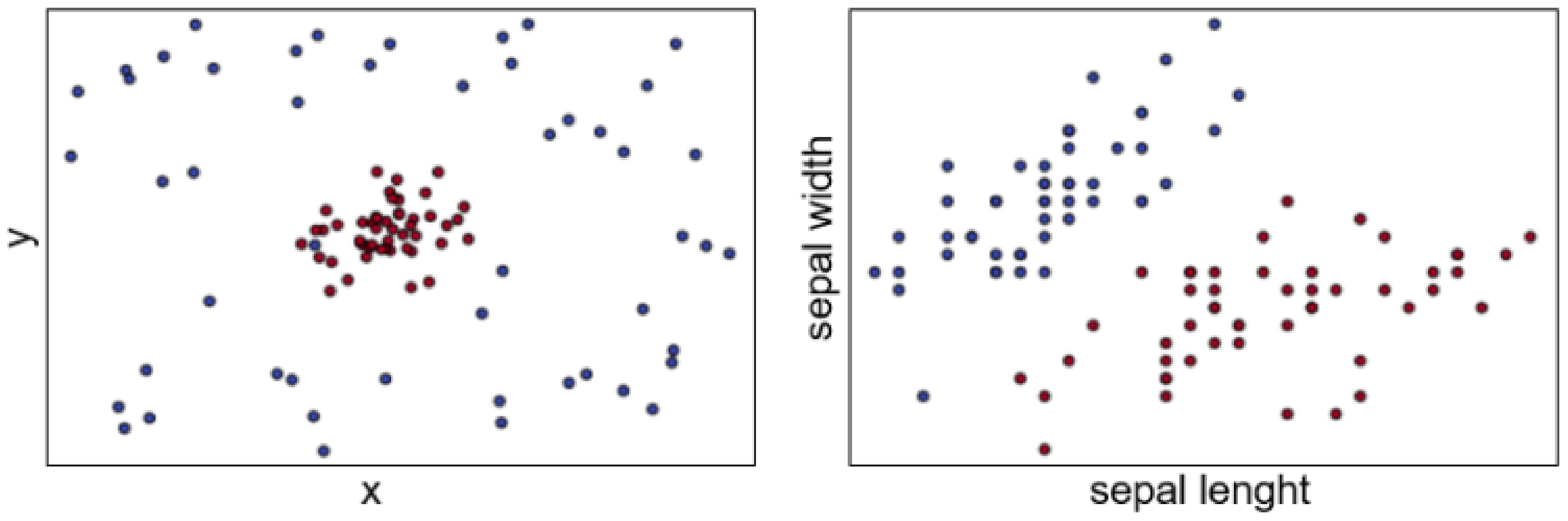
2.1. Synthetic Data
2.2. Iris Data
2.3. Indian Pine HSI
2.4. PolSAR Image of San Francisco
3. Coresets of Our Datasets
4. Weighted Classical and Quantum SVMs on Our Coresets
4.1. Weighted Classical SVMs
4.2. Weighted Quantum SVMs
5. Our Experiments
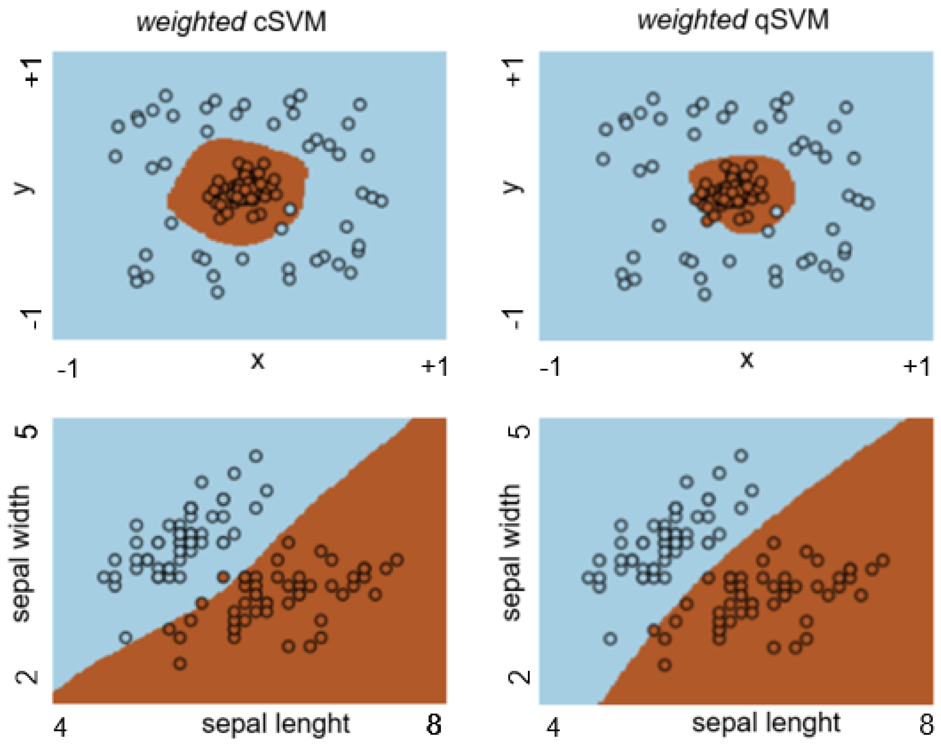
5.1. Synthetic Two-Class Data and Iris Data
- Annealing time: We controlled the annealing time by an anneal schedule. The anneal schedule is defined by the four series of pairs defined in (21). We set the annealing schedule accordingly:
- Number of reads: 10,000
- Chain strength: 50.
5.2. Indian Pine HSI and PolSAR Image of San Francisco
6. Discussion and Conclusions
Author Contributions
Funding
Institutional Review Board Statement
Informed Consent Statement
Data Availability Statement
Acknowledgments
Conflicts of Interest
References
- Richards, J. Remote Sensing Digital Image Analysis; Springer: Berlin/Heidelberg, Germany, 2013. [Google Scholar] [CrossRef]
- Cheng, G.; Xie, X.; Han, J.; Guo, L.; Xia, G.S. Remote Sensing Image Scene Classification Meets Deep Learning: Challenges, Methods, Benchmarks, and Opportunities. IEEE J. Sel. Top. Appl. Earth Obs. Remote Sens. 2020, 13, 3735–3756. [Google Scholar] [CrossRef]
- LeCun, Y.; Bengio, Y.; Hinton, G. Deep learning. Nature 2015, 521, 436–444. [Google Scholar] [CrossRef]
- Marmanis, D.; Datcu, M.; Esch, T.; Stilla, U. Deep Learning Earth Observation Classification Using ImageNet Pretrained Networks. IEEE Geosci. Remote Sens. Lett. 2016, 13, 105–109. [Google Scholar] [CrossRef] [Green Version]
- Manousakas, D.; Xu, Z.; Mascolo, C.; Campbell, T. Bayesian Pseudocoresets. In Advances in Neural Information Processing Systems; Larochelle, H., Ranzato, M., Hadsell, R., Balcan, M.F., Lin, H., Eds.; Curran Associates, Inc.: New York, NY, USA, 2020; Volume 33, pp. 14950–14960. [Google Scholar]
- Campbell, T.; Beronov, B. Sparse Variational Inference: Bayesian Coresets from Scratch. In Advances in Neural Information Processing Systems; Wallach, H., Larochelle, H., Beygelzimer, A., d’Alché-Buc, F., Fox, E., Garnett, R., Eds.; Curran Associates, Inc.: New York, NY, USA, 2019; Volume 32. [Google Scholar]
- Campbell, T.; Broderick, T. Bayesian Coreset Construction via Greedy Iterative Geodesic Ascent. arXiv 2018, arXiv:1802.01737. [Google Scholar]
- Tukan, M.; Baykal, C.; Feldman, D.; Rus, D. On Coresets for Support Vector Machines. arXiv 2020, arXiv:2002.06469. [Google Scholar]
- Harrow, A.W. Small quantum computers and large classical data sets. arXiv 2020, arXiv:2004.00026. [Google Scholar]
- Tomesh, T.; Gokhale, P.; Anschuetz, E.R.; Chong, F.T. Coreset Clustering on Small Quantum Computers. Electronics 2021, 10, 1690. [Google Scholar] [CrossRef]
- Preskill, J. Quantum Computing in the NISQ era and beyond. Quantum 2018, 2, 79. [Google Scholar] [CrossRef]
- Denchev, V.S.; Boixo, S.; Isakov, S.V.; Ding, N.; Babbush, R.; Smelyanskiy, V.; Martinis, J.; Neven, H. What is the Computational Value of Finite-Range Tunneling? Phys. Rev. X 2016, 6, 031015. [Google Scholar] [CrossRef]
- Dunjko, V.; Briegel, H.J. Machine learning & artificial intelligence in the quantum domain: A review of recent progress. Rep. Prog. Phys. 2018, 81, 074001. [Google Scholar] [CrossRef] [Green Version]
- Rebentrost, P.; Mohseni, M.; Lloyd, S. Quantum Support Vector Machine for Big Data Classification. Phys. Rev. Lett. 2014, 113, 130503. [Google Scholar] [CrossRef]
- Huang, H.Y.; Broughton, M.; Mohseni, M.; Babbush, R.; Boixo, S.; Neven, H.; McClean, J.R. Power of data in quantum machine learning. Nat. Commun. 2021, 12, 2631. [Google Scholar] [CrossRef]
- Biamonte, J.; Wittek, P.; Pancotti, N.; Rebentrost, P.; Wiebe, N.; Lloyd, S. Quantum machine learning. Nature 2017, 549, 195–202. [Google Scholar] [CrossRef]
- Otgonbaatar, S.; Datcu, M. Natural Embedding of the Stokes Parameters of Polarimetric Synthetic Aperture Radar Images in a Gate-Based Quantum Computer. IEEE Trans. Geosci. Remote Sens. 2021, 1–8. [Google Scholar] [CrossRef]
- Otgonbaatar, S.; Datcu, M. Classification of Remote Sensing Images with Parameterized Quantum Gates. IEEE Geosci. Remote Sens. Lett. 2021, 1–5. [Google Scholar] [CrossRef]
- Boothby, K.; Bunyk, P.; Raymond, J.; Roy, A. Next-Generation Topology of D-Wave Quantum Processors. arXiv 2020, arXiv:2003.00133. [Google Scholar]
- Farhi, E.; Goldstone, J.; Gutmann, S.; Sipser, M. Quantum Computation by Adiabatic Evolution. arXiv 2000, arXiv:0001106. [Google Scholar]
- Cavallaro, G.; Willsch, D.; Willsch, M.; Michielsen, K.; Riedel, M. Approaching Remote Sensing Image Classification with Ensembles of Support Vector Machines on the D-Wave Quantum Annealer. In Proceedings of the IGARSS 2020–2020 IEEE International Geoscience and Remote Sensing Symposium, Waikoloa, HI, USA, 26 September–2 October 2020; pp. 1973–1976. [Google Scholar] [CrossRef]
- Otgonbaatar, S.; Datcu, M. A Quantum Annealer for Subset Feature Selection and the Classification of Hyperspectral Images. IEEE J. Sel. Top. Appl. Earth Obs. Remote Sens. 2021, 14, 7057–7065. [Google Scholar] [CrossRef]
- Shang, F.; Hirose, A. Quaternion Neural-Network-Based PolSAR Land Classification in Poincare-Sphere-Parameter Space. IEEE Trans. Geosci. Remote Sens. 2014, 52, 5693–5703. [Google Scholar] [CrossRef]
- Cloude, S.R.; Papathanassiou, K.P. Polarimetric SAR interferometry. IEEE Trans. Geosci. Remote Sens. 1998, 36, 1551–1565. [Google Scholar] [CrossRef]
- Willsch, D.; Willsch, M.; De Raedt, H.; Michielsen, K. Support vector machines on the D-Wave quantum annealer. Comput. Phys. Commun. 2020, 248, 107006. [Google Scholar] [CrossRef]
- Lee, J.S.; Boerner, W.M.; Schuler, D.; Ainsworth, T.; Hajnsek, I.; Papathanassiou, K.; Lüneburg, E. A Review of Polarimetric SAR Algorithms and their Applications. J. Photogramm. Remote. Sens. China 2004, 9, 31–80. [Google Scholar]
- Moreira, A.; Prats-Iraola, P.; Younis, M.; Krieger, G.; Hajnsek, I.; Papathanassiou, K. A Tutorial on Synthetic Aperture Radar. IEEE Geosci. Remote Sens. Mag. (GRSM) 2013, 1, 6–43. [Google Scholar] [CrossRef] [Green Version]
- Sheykhmousa, M.; Mahdianpari, M.; Ghanbari, H.; Mohammadimanesh, F.; Ghamisi, P.; Homayouni, S. Support Vector Machine Versus Random Forest for Remote Sensing Image Classification: A Meta-Analysis and Systematic Review. IEEE J. Sel. Top. Appl. Earth Obs. Remote Sens. 2020, 13, 6308–6325. [Google Scholar] [CrossRef]
- Yang, X.; Song, Q.; Cao, A. Weighted support vector machine for data classification. In Proceedings of the 2005 IEEE International Joint Conference on Neural Networks, Montreal, QC, Canada, 31 July–4 August 2005; Volume 2, pp. 859–864. [Google Scholar] [CrossRef]
- Otgonbaatar, S.; Datcu, M. Quantum annealer for network flow minimization in InSAR images. In Proceedings of the EUSAR 2021: 13th European Conference on Synthetic Aperture Radar, Online. 29 March–1 April 2021; pp. 1–4. [Google Scholar]
- Pedregosa, F.; Varoquaux, G.; Gramfort, A.; Michel, V.; Thirion, B.; Grisel, O.; Blondel, M.; Prettenhofer, P.; Weiss, R.; Dubourg, V.; et al. Scikit-learn: Machine Learning in Python. J. Mach. Learn. Res. 2011, 12, 2825–2830. [Google Scholar]


| Synthetic Data | Iris Data | |
|---|---|---|
| Classes | {setosa, versicolour} | |
| Data size | 100 | 100 |
| Indian Pine HSI | ||||||
|---|---|---|---|---|---|---|
| Classes | ||||||
| Data size | 295 | 452 | 214 | 144 | 243 | 758 |
| PolSAR Image of San Francisco | ||
|---|---|---|
| Classes | {urban area, sea water} | {vegetation, sea water} |
| Data size | 61,465 | 61,465 |
| Classes | Data Size | Coreset Size | KL Divergence |
|---|---|---|---|
| 100 | 20 | 0.008194 | |
| {setosa, versicolour} | 100 | 22 | 0.053002 |
| {1, 2} | 295 | 79 | 0.573451 |
| {2, 3} | 452 | 56 | 0.003121 |
| {3, 4} | 214 | 33 | 0.000600 |
| {4, 5} | 144 | 41 | 0.017201 |
| {5, 6} | 243 | 41 | 0.001823 |
| {6, 7} | 758 | 125 | 0.492636 |
| {urban area, sea water} | 61,465 | 501 | 0.125072 |
| {vegetation, sea water} | 61,465 | 343 | 0.272749 |
| Classes | Coreset Size | Qacc | Cacc |
|---|---|---|---|
| 20 | 0.95 | 0.97 | |
| {setosa, versicolour} | 22 | 0.99 | 0.98 |
| {1, 2} | 79 | 0.96 | 0.96 |
| {2, 3} | 56 | 0.70 | 0.70 |
| {3, 4} | 33 | 0.88 | 0.88 |
| {4, 5} | 41 | 0.78 | 0.78 |
| {5, 6} | 41 | 0.71 | 0.71 |
| {6, 7} | 125 | 0.92 | 0.90 |
| {urban area, sea water} | 501 | 0.99 | 0.98 |
| {vegetation, sea water} | 343 | 0.99 | 0.99 |
Publisher’s Note: MDPI stays neutral with regard to jurisdictional claims in published maps and institutional affiliations. |
© 2021 by the authors. Licensee MDPI, Basel, Switzerland. This article is an open access article distributed under the terms and conditions of the Creative Commons Attribution (CC BY) license (https://creativecommons.org/licenses/by/4.0/).
Share and Cite
Otgonbaatar, S.; Datcu, M. Assembly of a Coreset of Earth Observation Images on a Small Quantum Computer. Electronics 2021, 10, 2482. https://doi.org/10.3390/electronics10202482
Otgonbaatar S, Datcu M. Assembly of a Coreset of Earth Observation Images on a Small Quantum Computer. Electronics. 2021; 10(20):2482. https://doi.org/10.3390/electronics10202482
Chicago/Turabian StyleOtgonbaatar, Soronzonbold, and Mihai Datcu. 2021. "Assembly of a Coreset of Earth Observation Images on a Small Quantum Computer" Electronics 10, no. 20: 2482. https://doi.org/10.3390/electronics10202482
APA StyleOtgonbaatar, S., & Datcu, M. (2021). Assembly of a Coreset of Earth Observation Images on a Small Quantum Computer. Electronics, 10(20), 2482. https://doi.org/10.3390/electronics10202482